Prologue: smooth approximation

(1)

Linac 10-Tsukuba

A.Pisent RFQ for cw applications

Prologue: smooth

approximation

Andrea Pisent

(2)

Istituto Nazionale di Fisica Nucleare (Italy) A.Pisent RFQ for cw applications Linac 10-Tsukuba

Smooth approximation

The general idea is that for a Hill equation:

) ( ) ( 0 ) ( " K s x K s L K s x     (1)

we want an approximate solution of pendulum kind:

       L z a x ₀sin ₀ (2)

by applying some averaging. The problem is not completely trivial since the average of the force is null:



  L dz z K L K 0 0 ) ( 1 (3)  0 180    54.61705  180    54.61705 2 0 2   2  180    109.23411 _ ₀ 2 _ ₃__ 2 180    109.23411 0 2 4 6 8 10 2  10  3 0 2 10  3 length s/L ,y ( ) y Z i1 Z i1  xsingola i kkk i kkk 0 axT 2  Z i0 T

(3)

The proof of smooth approximation is simple and powerful: we consider that the solution of the Hill equation can be written as the product of two terms, the first is fast and is periodic with L, the second is so slow that can be averaged on the period L. Namely:



1 q(s)



X(s) q(s L) q(s)

x     (11)

q(s)<<1 has the following proprieties:

) ( " 0 ) ( ' ) ( 0 0 K K q dz z q dz z q L L     



₍₁₂₎

The substitution of (11) into Hill’s equations (1) gives:

0 ) 1 ( ' ' 2 )) ( ( ) 1 ( " q  X  K K  X q K q X  X (13)

When we average this expression over a period, for the fast term averages following the (12), and we have that the only surviving terms give and harmonic oscillator equation for the slow term X:





0

" K  qK X 

X (14)

where we have now a phase advance defined also if K has average null (or negative, like a FODO with space charge or RF defocussing).

Let’s use these formulas in two important cases, the thin lens FODO above and a sinusoidal focusing channel (the RFQ). The FODO is coherent with the value from matrix calculation, namely the phase advance (8) and envelope modulation (10).

(4)

Smooth approximation for FODO and RFQ

K q  FODO )) 2 / ( ) ( ( 1 ) ( z z L f z K                         2 2 2 1 8 2 2 8 ) ( L z L z f f L L z f z f L z q 2 2 2 4 f L   RFQ K()  Bcos2    cos2 4 ) ( B₂ q  2 2 2 8   B 0180   29.55545 180   14.48187 2022 180   46.54566 _₀2_₃__2180   38.76466 0 5 10 15 20 25 30 35 40 45 50 0.002 0 0.002 length s/L ax, ay K (s ) arbitrary s cale Zi 1 Zi 3  kkki kkk0 axT 2  asmooth Zi 0 T    bsmooth Zi 0 T     Zi 0 T

With space charge and RF defocusing

2 2 2 2 0 2

2

2 a

L

RF













0 "



K



qK

X



X

(5)

Smooth approximation of a FODO lattice

F 0 D 0 L/2 L/2     sin 2 sin 1    L a

(6)

(7)

The problem of capture efficiency in a linac

• Starting with a continuous mono energetic beam from source, only particles in the separatrix will be captured.

• Typically if



₀=-200 _only

60/360=17% of particles will be captured

• Something must be invented, especially for high intensity or for rare ion beams.

o



3

(8)

Istituto Nazionale di Fisica Nucleare (Italy) A.Pisent RFQ for cw applications Linac 10-Tsukuba d

Buncher (gap+drift)

4 2 0 2 4 0.1 0 0.1 dw2_nn d1_nn 4 2 0 2 4 0.1 0 0.1 dw2_nn d2_nn 100 75 50 25 0 25 50 75 100 4 3 2 1 0 1 2 3 4 3.142 3.142  d2nn 30 180 30 180     100 100  d0_nn  100 _buncher _linac _buncher _linac

After the bunching cavity the longitudinal phase distribution Evolves with a density peak at the wanted phase.

(9)

d

Buncher (gap+drift)

4 2 0 2 4 0.1 0 0.1 dw2_nn d1_nn 4 2 0 2 4 0.1 0 0.1 dw2_nn d2_nn 100 75 50 25 0 25 50 75 100 4 3 2 1 0 1 2 3 4 3.142 3.142  d2nn 30 180 30 180     100 100  d0_nn  100 _buncher _linac _buncher _linac

After the bunching cavity the longitudinal phase distribution Evolves with a density peak at the wanted phase.

(10)

d

Buncher (gap+drift) Two harmonics

100 75 50 25 0 25 50 75 100 4 3 2 1 0 1 2 3 4 3.142 3.142  d2nn 30 180 30 180     100 100  d0_nn  100 4 2 0 2 4 0.2 0 0.2 0.13 0.13  dw2nn 3.142 3.142  d1nn _buncher _linac _buncher _ linac

About 75% efficiency can be reached

4 2 0 2 4 0.2 0 0.2 0.13 0.13  dw2nn 3.142 3.142  d2_nn _linac

(11)

Beam dynamics in RFQ

linear accelerators

Andrea Pisent

(12)

outline

• Wikipedia RFQ “invented by Soviet physicists I. M. Kapchinsky and

Vladimir Teplyakov in 1970, the RFQ is presently used as an injector by major laboratories and industries throughout the world for

radiofrequency linear accelerators.[2]”

• Main features

– RF acceleration at low energy / replace the high voltage injectors – Adiabatic bunching / high capture efficiency

(13)

RFQs replace with RF linac electrostatic injectors

example CERN RFQ2

(14)

Fusion Material Irradiation Test Project - FMIT a US Department of Energy project,

accepted as a necessary and vital element for the development of fusion power.

• Construction project approved 1975

• Accelerator construction undertaken by new Accelerator Technology Division at Los Alamos January 1978, after discussions in 1977.

• No IF’s firm budget and schedule, BUT huge R&D question

-injection of 100 mA cw into DTL required several 100 kV DC injector. • Discovery of Teplyakov RFQ work in Russia.

• Proposal to DOE for RFQ development, approved!

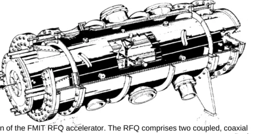
Courtesy of R. Jameson Fig. 1. Initial design of the FMIT RFQ accelerator. The RFQ comprises two coupled, coaxial

resonators. The rf power is loop coupled into the outer section. or manifold, which more uniformly distributes the power into the four quadrants of the inner resonator, or core. A 75keV beam is

injected (arrow, left in the figure) and accelerated to 2 MeV.

(15)

RFQs general parameters

Name Lab ion energy vane beam RF Cu Freq. length Emax Power density

voltage current power power ave max

MeV/u k V mA k W k W MHz m lambda k ilpat W/cm2 W/cm2

IFMIF EVEDA LNL d 2.5 79-132 130 650 585 175 9.8 5.7 1.8 3.5 60

pulsed CERN linac 2 CERN p 0.75 178 200 150 440 202 1.8 1.2 2.5

SNS LBNL H- 2.5 83 70 175 664 402.5 3.7 5.0 1.85 1.1 10

CERN linac 3 LNL A/q=8.3 0.25 70 0.08 0.04 300 101 2.5 0.8 1.9

CW LEDA LANL p 6.7 67-117 100 670 1450 350 8 9.3 1.8 11.4 65

FMIT LANL d 2 185 100 193 407 80 4 1.0 1 0.4

high p IPHI CEA p 3 87-123 100 300 750 352 6 7.0 1.7 15 120

TRASCO LNL p 5 68 30 150 847 352 7.3 8.6 1.8 6.6 90

CW SARAF NTG d 1.5 65 4 12 250 176 3.8 2.2 1.6

mid p SPIRAL2 CEA A/q=3 0.75 100-113 5 7.5 170 88 5 1.5 1.65 0.6 19

CW ISAC TRIUMF A/q=30 0.15 74 0 0 150 35 8 0.9 1.15 -

-lp PIAVE LNL A/q=6 0.58 280 0 0 8e-3 (SC) 80 2.1 0.5 - -

-IFMIF-EVEDA RFQ

• 18 modules 9.8 m

• Powered by eight 220 kW rf chains and 8 couplers

• High availability 30 years operation.

• Hands on maintenance

• First complete installation in Japan (Rokkasho site)

The RFQ is

INFN Italy responsibility LNL

Padova Torino ..Bologna

(16)

(17)

A. Pisent "Introduzione alle Macchine acceleratrici " 2007



E

v

B



e

dt

p

d









(18)

The field between electrodes can be calculated in quasi static approximation. The general solution of Laplace equation in cylindrical coordinates is:





                            



n n m n nm n nr n A I kr n mkz A V z r r r r r z t z r E , 2 2 0 2 2 2 2 2 2 2 cos 2 cos ) ( 2 cos 2 ) , , ( 0 1 1 ) cos( ) , , (        

NB already encontered yesterday for magnetic quadrupoles (n=1) and RF gap (order n=0). To accelerate and focus we need again these two terms:

With k. The electrods correspond to the equipotentials . For z=0

Have the minimum aperture (called a) in x plane and the maximum aperture (called ma in the y

plane; m>1 (modulation factor) is a real number (nothing to do with mass)

Electrode modulation



A r A I kr kz



V z r cos2 ( )cos 2 ) , , ( 2 ₁₀ ₀ 01      2 ) , , (r z V  









2 ) ( 2 ) 0 , 2 , ( 2 ) ( 2 ) 0 , 0 , ( 0 10 2 2 01 0 10 2 01 V mka I A a m A V ma V ka I A a A V a           

(19)

The field between electrodes can be calculated in quasi static approximation. The general solution of Laplace equation in cylindrical coordinates is:





                            



n n m n nm n nr n A I kr n mkz A V z r r r r r z t z r E , 2 2 0 2 2 2 2 2 2 2 cos 2 cos ) ( 2 cos 2 ) , , ( 0 1 1 ) cos( ) , , (        

NB already encontered yesterday for magnetic quadrupoles (n=1) and RF gap (order n=0). To accelerate and focus we need again these two terms:

With k. The electrods correspond to the equipotentials . For z=0

Have the minimum aperture (called a) in x plane and the maximum aperture (called ma in the y

plane; m>1 (modulation factor) is a real number (nothing to do with mass)

Electrode modulation



A r A I kr kz



V z r cos2 ( )cos 2 ) , , ( 2 ₁₀ ₀ 01      2 ) , , (r z V  









2 ) ( 2 ) 0 , 2 , ( 2 ) ( 2 ) 0 , 0 , ( 0 10 2 2 01 0 10 2 01 V mka I A a m A V ma V ka I A a A V a           

(20)

h

                          2 0 0 2 0 0 0 2 01 0 2 0 2 10 0 10 2 2 01 0 10 2 01 1 ) ( ) ( ) ( ) ( 1 ) ( ) ( 1 1 ) ( 1 ) ( R ka I m mka I ka I mka I a A A ka I m mka I m A mka I A a m A ka I A a A

The vane profile is only approximately sinusoidal:

kz kx AI R x cos ) ( 2 ₂ ₀ 0 2  

The electrodes follow only approximately the two terms potential.

1. Does not extend as an hyperbola to infinity

2. The radius of vane tip is constant (and generally less than R₀ to limit the surface field).

The modulation factor m has to be enhanced to get the necessary acceleration.

In the computer simulation the field applied includes the higher order components



(21)

Equations of motion

From the two terms potential

          A I kr kz R y x V z y x ( )cos 2 ) , , ( ₂ ₀ 0 2 2

The transverse and longitudinal equations (respect to the parameter ) read d  _dz





2 0 2 2 2 2 0 2 2 2 3 0 2 2 0 2 0 0

sin

4 )

(

sin

0

2 cos

cos

2 )

cos(

)

2 cos(

)

(

R

mc

eV

B

mc

eAV

mc

eE

K

x

K

B

d

x

d

eAV

z

dzE

e

d

dw

a RF RF z



























































(22)

Equations of motion





2 0 2 2 2 2 0 2 2 2 3 0 2 2 0 2 0 0

sin

4 )

(

sin

0

2 cos

cos

2 )

cos(

)

2 cos(

)

(

R

mc

eV

B

mc

eAV

mc

eE

K

x

K

B

d

x

d

eAV

z

dzE

e

d

dw

a RF RF z



























































focussing acceleration focussing acceleration

(23)

Equations of motion





2 0 2 2 2 2 0 2 2 2 3 0 2 2 0 2 0 0

sin

4 )

(

sin

0

2 cos

cos

2 )

cos(

)

2 cos(

)

(

R

mc

eV

B

mc

eAV

mc

eE

K

x

K

B

d

x

d

eAV

z

dzE

e

d

dw

a RF RF z



























































focussing acceleration focussing acceleration Focussing factor

(24)

Parameters dependence: A

acceleration

Freg 0₁ _1.5 ₂ _2.5 ₃ 0.2 0.4 0.6 0.8 A x .8(  ) A x ..6(  ) A x .4(  ) A x .2(  ) A x 0(  ) x21 x21 m m ka





a

ka

m

ka

I

m

mka

I

m

ka

m

A

_ka

2

1

1 )

(

)

(

1 )

,

(

₂ 2 0 0 2 0 2









 









_

(25)

Parameters dependence:

average aperture R

₀

m m R0/a

2

1 )

(

)

(

)

(

)

(

)

,

(

0 0 0 2 0 0







m

ka

I

mka

I

ka

I

m

mka

I

ka

m

a

R

R0/a 1 1.5 2 2.5 3 1 1.5 2 2.5 chi x .8(  ) chi x .6(  ) chi x .4(  ) chi x .2(  ) chi x 0( ) x 1 2 x 1 1.5 2 2.5 3 0.8 0.9 1 1.1 1.2 chinorm x .8(  ) chinorm x .6(  ) chinorm x .4(  ) chinorm x .2(  ) chinorm x 0( ) x

(26)

Istituto Nazionale di Fisica Nucleare (Italy) A.Pisent RFQ for cw applications Linac 10-Tsukuba 1 1.5 2 2.5 3 0 0.05 0.1 0.15 0.2 EasuEs x .8(  ) EasuEs x .6(  ) EasuEs x .4(  ) EasuEs x .2(  ) EasuEs x 0(  ) x 0 1 2 3 0 0.05 0.1 0.15 EasuEs 1.5 ka  _jj EasuEs 2 ka  _jj EasuEs 3 ka  _jj

ka_jjchi 1.5 ka  _jjka_jjchi 2 ka  _jjka_jjchi 3 ka  _jj

Accelerating field vs surface field

• In new RFQs the field is generally increased at high energy to compensate the decrease of Ea with  typical of a constant voltage structure

kRo m 0 0 0 0 2 0 0 0 0 0 0 0 1 2 ) 2 ( 2 ) , ( ) , ( 4 ) , ( ) , ( 4 ) , ( R q AkR qkR I q kR m kR m kR m A kR E E R V kR m E kR m VkA AV E s a s a                    Ea/Es Ea dipendance with modulation Parameters

Es is the surface field

(27)

Transverse focussing vs surface field

• Concerning transverse

focusing there are two results • If a high B is needed (to

counteract RF defocussing or space charge) R0 and

therefore V must be reasonably low

• From the point of view of acceptance (to avoid losses on halo) it is convenient high voltage and large aperture.

V

m

B

R

a

kR

m

kR

m

A

kR

E

R

mc

e

E

B

R

mc

eV

B

R

V

kR

m

E

n s a s s

























2 2 0 2 0 0 0 0 2 2 2 0 2 2 0 0

1

2

8 )

,

(

4 )

,

(

)

,

(















(28)

Break

(29)

Beam dynamics: parameters period by

period

(30)

Istituto Nazionale di Fisica Nucleare (Italy) A.Pisent RFQ for cw applications Linac 10-Tsukuba Modulation “m”, average aperture “r0” [cm], small aperture “a” [cm], Voltage/100 [kV] E0 [MV/m], Acceleration factor “A10”, Energy “W”, Focusing “B”, ‐Sync. Phase/100 [deg], Pole tip “rho”, along the RFQ Shaper GB Accelerator Ions d

Energy range 0.1-5 MeV

input-output nom emitt 0.25 mmmrad (rms) Ouput long emitt. 0.2 MeV deg (rms) Output current 0.2

Tansmission 98 % WB distr. 95 % Gsussian distr.

(31)

(32)

Beam matching at the input

• The beam at RFQ input is

continous and has to be matched to a time-dependent focusing. The focusing has to rise adiabatically to allow the transverse capture

(33)

Bunching section

• Prepares the buch to be accelerated

• In the shaper A and _ are raised linearly to form the separatrix

• In the gentle buncher A and

₀ are raised keeping the sigmal (bunch length in space) and the separatrix area (to keep the captured particles)

Modulation “m”, average aperture “r0” [cm], small aperture “a” [cm], Voltage/100 [kV] E0 [MV/m], Acceleration factor “A10”, Energy “W”, Focusing “B”,

‐Sync. Phase/100 [deg], Pole tip “rho”, along the RFQ

(34)

(35)

accelerating section

• The field is ramped in the

accelerating section to

compensate the decrease of Ea with  typical of a

constant voltage structure.

• The increase is limited by the power per structure meter, and transverse acceptance.

Modulation “m”, average aperture “r0” [cm], small aperture “a” [cm], Voltage/100 [kV] E0 [MV/m], Acceleration factor “A10”, Energy “W”, Focusing “B”,

‐Sync. Phase/100 [deg], Pole tip “rho”, along the RFQ

(36)

Cavity cross section

12/06/2008 36 Wb Wb Beginning End 340 mm 173 173.5 174 174.5 175 175.5 0 200 400 600 800 1000 z axis [cm] Frequency [MHz] 0 1 2 3 4 5 Half Width Vane Base [cm] Frequency WBASE 0 50 100 150 200 250 300 0 200 400 600 800 1000 z axis [cm] Shunt Im peda nce [k  *m] 0 100 200 300 400 500 600 700 Po wer [W/c m ] Rs [kOhm*m] (4 quad) P [W/cm] 4 quad 2d simulation values

(37)

0.5 1 1.5 2 2.5 3 3.5 4 4.5 5 5.5 0 100 200 300 400 500 600 700 800 900 1000 A cce p tan ce [mmmra d ]; m; a [mm] RFQ Length [cm] Acce (mmmrad) m a (mm)

Acceptance increase in the accelerator part

Shaper GB Accelerator

(38)

Beam Loss [uA/m]

0 5 10 15 0 200 400 600 800 1000 z Cur re n t Lo ss [u A /m ] Series1 Beam Loss [W/m] 0 50 100 150 200 250 0 200 400 600 800 1000 z Pow e r Lo ss [W /m ] Series1

Neutron production estimate [n/(s*m)]

0.00E+00 5.00E+08 1.00E+09 1.50E+09 2.00E+09 0 200 400 600 800 1000 RFQ Length [cm] ne ut ro ns [n /( s* m )] Series1 RFQ Length [cm] Integral 1.4 mA Integral 3.8 10^9 n/s Integral 549 W

WB distribution 0.25 mm mrad rms norm 1 . 2 7 10 * 15 . 5 Nw n 

(39)

Effect of Input Current and beam distribution

Runs with TraceWin; emit=0.25 mmmrad RMS; Np=100000

(40)

The Phase Advance along the RFQ

I=0

I=130

(41)

Error studies

• The error study shows tolerances in beam alignment and electrode

displacements of the order of 0.1 mm, while the RF field law has to be

followed with an accuracy of 1-2%. • Example: displacement between two

modules (9 modules) 93.5 93.8 94.1 94.4 94.7 95 95.3 95.6 95.9 96.2 96.5 800 940 1080 1220 1360 1500 1640 1780 1920 2060 2200 0 10 20 30 40 50 60 70 80 90 100 Tr a n sm issi o n [% ] Po w er Lo ss [W a tts ]

Profile Max Error [um]

Gaussian Seg 550 mm

Power Loss min [W] Power Loss ave [W] Power Loss MAX [W] Tr [%] min Tr [%] ave Tr [%] MAX

Transmission and Power loss due to the segmentations applied with gaussian and waterbag input beam distribution.(TOUTATIS)

97.1 97.3 97.5 97.7 97.9 98.1 98.3 98.5 98.7 98.9 99.1 200 300 400 500 600 700 800 900 1000 1100 1200 0 10 20 30 40 50 60 70 80 90 100 Tr a n sm issi o n [% ] Pow er Lo ss [W atts ]

Profile Max Error [um]

WaterBag Seg 550 mm

Power Loss min [W] Power Loss ave [W] Power Loss MAX [W] Tr [%] min

Tr [%] ave Tr [%] MAX

(42)

(43)

CERN lead ion RFQ (Pb injector of LHC)

• A/q=208/25

• 100 uA Pb beam (pulsed low duty) • Energy range 2.5-250 keV/u

• Transmission 93% with large

multipole correction (kR₀=3.3, m=1.1) • Operational since 1994

• Built in Italy at De Pretto and Cinel • Linac 3 will inject Pb in LHC

• The linac 3 was built by an international collaboration (INFN-GANIL-GSI-CERN). • INFN LNL delivered in time and in specs

the LEBT the MEBT and the RFQ (except the RF, done by GSI)

(44)

Modulation in

Linac3 RFQ

• Respect to the high intensity

approach

• The aperture is kept quite large (B low) to increase acceleration

• there is a PB section, where the bunch is compressed fast at low energy.

• To bunch at low energy is very convenient for the length of the acceleartor.

• In the section called booster the aperture is closed up to specified one.

(45)

Modulation in

Linac3 RFQ

• Respect to the high intensity

approach

• The aperture is kept quite large (B low) to increase acceleration

• there is a PB section, where the bunch is compressed fast at low energy.

• To bunch at low energy is very convenient for the length of the acceleartor.

• In the section called booster the aperture is closed up to specified one.

(46)

Parametric

resonance has

been avoided

• In a preliminary dynamics the RFQ was shorter, but crossing the

condition

• Below are the stability limits of Mathiew equation

T

L



(47)

PIAVE SRFQ

The only superconducting RFQ operting in the world

Successfully in cw operation since 2006 at INFN • A/q=8.5 (used up to 7)

• 5 uA cw current

• Energy range 37-585 keV/u

• Large modulation factor (m up to 3) and intervane voltage (up to 280kV)

• Transmission 60% with external bunching • Operational since 2006

• Built in Italy at INFN (Nb electrodes machining) and Zanon.

(48)

RFQ functions

charge number 28 mass number 238 Injection platform 315 kV SRFQ #1 SRFQ #2 in out in out Energy 37.1 351.3 585.4 keV/u 8.82 83.61 139.33 MeV Beta  0.0089 0.0275 0.0355 Voltage 148.0 148.0 280.0 280.0 kV Length 138.9 74.4 cm Ncell 43 13 m 1.2 2.8 2.7 2.8 a 0.7 0.4 0.8 0.8 cm R0 0.80 0.80 1.53 1.53 cm Phis  40.0 18.0 12.0 12.0 deg

Max. Surface field 24.1 24.0 MV/m

Stored energy 1.8 3.5 J

Total length 213.27 cm (TTF in the first QWR=

0.87

Eq. voltage 4.66 MV

Average acc. 2.19 MV/m

(49)

• The physical distance between the two SRFQs (200mm) determines a transverse beam mismatch in

SRFQ2 (where the acceptance is large).

• This mismatch has been minimized interrupting SRFQ1 in a point

where the Twiss parameter are

_x=_y=0. 200 746 Scala 1:10 1378 SRFQ2 SRFQ1

Servizio UFFICIO TECNICO

half cell terminati on

(50)

• The physical distance between the two SRFQs (200mm) determines a transverse beam mismatch in

SRFQ2 (where the acceptance is large).

• This mismatch has been minimized interrupting SRFQ1 in a point

where the Twiss parameter are

_x=_y=0. Z3i 1 Z3i 3 kkk3i kkk30 axT 2  Z3i 0 T 0 1 2 3 4 5 6 7 8 9 10 0.005 0 0.005 B eam en ve lo pe s [arb itrary scale] Z2i 1 Z2i 3 kkki kkk0 axT 2  Z2i 0 T 0 1 2 3 4 5 6 7 8 9 10 0.005 0 0.005 z B eam en ve lo pe [arb itrary scale] - vertical envelope Horizontal envelope transmission 0 0.2 0.4 0.6 0.8 1 1.2 0 0.3 0.5 0.7 0.9 1.2

Input Norm. Em ittance [mm mra d]

T ran sm is si o n s trans.SRQ1 trans. SRFQ2 trans SRFQ2 half-cell Nominal 200 746 Scala 1:10 1378 SRFQ2 SRFQ1

Servizio UFFICIO TECNICO

half cell terminati on

(51)

RFQ emittance

ECR buncher SRFQs QWRs buncher buncher ALPI



_x

+



_y

B

44 channels 1: Transverse NormalizedEmittance at SRFQs exit.

Ion Ε_RMS,x [mm-mrad] Ε_RMS,y [mm-mrad]

40_Ar9+_0.10 _0.10

16_O3+_0.11 _0.12

(52)

Conclusions

• The beam dynamics of an RFQ is written once for ever in the

metal.

– The designer has the choice of modulation parameters in some hundreds of modulation periods.

– This flexibility allows different approaches and very optimized accelerators for many specific high performance applications.

• BUT

– Once built the RFQ is not flexible at all, since very few parameters can be changed in operation.

– The construction has to follow strict tolerances (important technological challenges related to construction and RF tuning).

– One has to relay on computer simulations and design approaches, since experimental verification of the correctness of the design arrives after many years.

(53)

Name Lab ion energy vane beam RF Cu Freq. length Emax Power density operate

IFMIF EVEDA LNL d 2.5 79-132 130 650 585 175 9.8 5.7 1.8 3.5 60 NO

p p_p

CW SARAF NTG d 1.5 65 4 12 250 176 3.8 2.2 1.4 24 190 only p

RFQ four rods or four vanes

IFMIF-EVEDA SARAF at SOREQ (Israel)

• Smaller cross section and dipoles at higher frequency.

• Diffused hot spots

• Better shunt impedance, possibility to reach high voltage

• Larger dimensions, dipole stop band to master

(54)

Name Lab ion energy vane beam RF Cu Freq. length Emax Power density operate

IFMIF EVEDA LNL d 2.5 79-132 130 650 585 175 9.8 5.7 1.8 3.5 60 NO

p p_p

CW SARAF NTG d 1.5 65 4 12 250 176 3.8 2.2 1.4 24 190 only p

RFQ four rods or four vanes

IFMIF-EVEDA SARAF at SOREQ (Israel)

• Smaller cross section and dipoles at higher frequency.

• Diffused hot spots

• Better shunt impedance, possibility to reach high voltage

• Larger dimensions, dipole stop band to master

(55)

Questions

1. What is the field of application of Radio Frequency Quadrupoles? 2. Why for RFQ it is convenient to focus transversally with an electric

field?

3. What is the modulation factor m and which is the effect to encrease it?

4. Why in a RFQ it is possible to bunch the beam with a very high efficiency?

5. Why at higher energy it is convenient to increase the intervane voltage along the RFQ?

6. Why an RFQ in the case of negligible space charge can be shorter? 7. For an RFQ (already in operation) by increasing the voltage, how

does the output energy change (in first approximation)?

8. If during the design the input energy is decreased, what happens to the RFQ length (for similar bunching law)?