Optimization of Mixed Fare Structures:
Theory and Applications
Received (in revised form): 7th April 2009
Thomas Fiig
is Chief Scientist in the Revenue Management Development department at Scandinavian Airlines System (SAS). He is responsible for developing methods and strategy for revenue management systems at SAS, including the overall design and methodologies of the O&D forecasting and optimization systems. His recent work has focused on methodologies for O&D optimization in semi-restricted fare structures and estimating price elasticities. Dr Fiig holds a PhD in Mathematics and theoretical Physics and a BA in Finance from the University of Copenhagen.
Karl Isler
is Head of Operations Research and Strategy in the Revenue Management, Pricing and Distribution department of Swiss International Airlines. He holds a PhD in Theoretical Physics from ETH Zurich. He developed the concepts for the integrated O&D pricing and inventory control strategy used by Swiss. Craig Hopperstad
is currently president of Hopperstad Consulting. Previously, as Project Director in the Boeing Commercial Airplane Group, he was a principal in the development of passenger preference, fleet planning, scheduling and revenue management models. He is the author of numerous papers and presentations, many of which deal with the application of the Passenger Origin/Destination Simulator (PODS), which he developed at Boeing and for which Hopperstad Consulting now holds a license.
Peter Belobaba
is Principal Research Scientist at the Massachusetts Institute of Technology (MIT), where he teaches graduate courses on The Airline Industry and Airline Management. He is Program Manager of MIT’s Global Airline Industry Program and Director of the MIT PODS Revenue Management Research Consortium. Dr Belobaba holds a Master of Science and a PhD in Flight Transportation Systems from MIT. He has worked as a consultant on revenue management systems at over 40 airlines and other companies worldwide.
Correspondence:Peter Belobaba, MIT International Center for Air Transportation, 77 Mass. Ave., Room 33–215, Cambridge, MA 02139 USA
E-mail: [email protected]
ABSTRACT This paper develops a theory for optimizing revenue through seat inventory control that can be applied in a variety of airline fare structures, including those with less restricted and fully undifferentiated fare products that have become more common in the recent past. We describe an approach to transform the fares and the demand of a general discrete choice model to an equivalent independent demand model. The transformation and resulting fare adjustment approach is valid for both static and dynamic optimization and extends to network revenue management applications. This transformation allows the continued use of the optimization algorithms and seat inventory control mechanisms of traditional revenue management systems, developed more than two decades ago under the assumption of independent demands for fare classes. Journal of Revenue and Pricing Managementadvance online publication, 19 June 2009; doi:10.1057/rpm.2009.18
Keywords:seat inventory control; airline fare structures; network revenue maximization; O-D control; marginal revenue transformation; DAVN-MR, PODS
INTRODUCTION AND
MOTIVATION
Traditional airline revenue management (RM) systems, developed in the late 1980s, make use of forecasting and optimization models that assume independent demands for each fare class on a flight leg, and/or for each passenger itinerary (path) and fare class in an airline network. This assumption of demand indepen-dence was facilitated by airline fare structures characterized by multiple fare products, each with different restrictions such as minimum stay requirements, advance booking and tick-eting rules, cancellation and change penalties, as well as non-refundability conditions. That is, passengers that purchase a given fare type are assumed to be willing to purchase only that particular fare type, with no possibility of choosing a lower fare, another itinerary (path) or another airline. Although this assumption of demand independence was never completely accurate, virtually all airline RM forecasting and optimization models were developed on this basis.
With changes to airline pricing practices in recent years, what was a questionable yet tolerable assumption for RM models became almost completely invalid. The emergence and rapid growth of low cost carriers (LCC) with less restricted fare structures has led to the introduction of a variety of ‘simplified’ fare structures with fewer restrictions and in some cases no restrictions at all. Without modifica-tions to traditional RM forecasting and optimi-zation models, along with their associated seat inventory control mechanisms, less restricted fare structures result in more passengers (higher load factors) purchasing lower fares (lower yields), but lower total revenues for the airline.
This paper develops a theory for optimizing revenue through seat inventory control in a completely arbitrary airline fare structure. Examples that will be considered here include independent product-oriented demand (also known as ‘yieldable’ demand) in traditional differentiated fare structures; price-oriented (that is, ‘priceable’) demand with
undifferen-tiated fares; and hybrid demand in fare structures with a mixture of differentiated and undifferentiated fare products.
The applicability of this approach to any fare structure (and hence the associated passenger choice demand) might suggest that the optimi-zation theory is complex.On the contrary– we will derive a marginal revenue transformation of the fares and the choice demand to an equivalent independent demand model. This transformation allows the continued use of existing optimization algorithms and control mechanisms in traditional RM systems. The marginal revenue transformation can be applied to all existing leg-based and O-D control RM systems, including EMSRb leg-based con-trol, Displacement Adjusted Virtual Nesting (DAVN) and Dynamic Programming (DP), as will be illustrated.
This paper restricts its discussion to the opti-mization theory and thus assumes that we are able through some other means to forecast the demand of the choice of fare products in each fare structure, as affected by both passenger will-ingness to pay and the RM system’s inventory controls. Demand forecasts that reflect fare pro-duct choice require the estimation of demand elasticity and sell-up parameters using separate estimation models, as described in Hopperstad (2007) and Guo (2008), for example.
The contribution of this paper is therefore in the presentation of a new theory for revenue management optimization that can be applied to any airline fare structure. The practical importance of this contribution is substantial – use of this new optimization theory can allow airlines to continue using traditional RM systems and seat inventory control mechanisms originally developed under the assumption of independent fare product demands.
After a brief review of relevant revenue management literature in the next section, we define the current optimization problem in the subsequent section and present a general formulation in the section after that. We first assume a number of simplifications: static optimization (no time dependence),
determi-nistic demand (no stochasticity), single airline leg (no network) and a single market (one specific price-demand relation). The theory is by no means limited by any of these simplifica-tions, which are only introduced to present the theory more clearly. We then discuss specific applications of the optimization theory to different fare structures. In the section ‘Exten-sions to stochastic models’ we show that the theory extends beyond the simplifications made above to stochastic models, including dynamic programming. Simulated revenue results from the Passenger Origin Destination Simulator (PODS) are presented in the section ‘Simula-tion results using PODS’.
LITERATURE REVIEW
Most revenue management techniques were developed under a critical assumption that demand for a given fare class is independent of the demand for other fare classes. The effective use of these revenue management (RM) systems by airlines worldwide has been estimated to generate on the order of 4–6 per cent in incremental revenues (Smith et al, 1992). Barnhart et al (2003) describe the evolution of revenue management systems since the early 1980s. McGill and van Ryzin (1999) provide a comprehensive survey of revenue management literature, focusing on the evolu-tion of forecasting and optimizaevolu-tion models.
The optimization of airline seat inventory to maximize revenue given multiple fare products on a single flight leg can be traced back to Littlewood (1972), who solved the fare class mix problem for two nested fare classes. Belobaba (1987, 1989) extended the nested seat allocation problem to multiple fare classes with the development of the Expected Marginal Seat Revenue (EMSR) heuristic. Curry (1990), Wollmer (1992) and Brumelle and McGill (1993) described optimal solutions for multiple nested fare classes. Belobaba (1992) then modified the EMSR heuristic to better approximate the optimal solution to the multi-ple nested fare class problem. The modified
version became known as ‘EMSRb’, and is also described in detail in Belobaba and Weath-erford (1996). Dynamic programming models have also been applied to the single-leg seat inventory control problem, by Lee and Hiersch (1993) and Lautenbacher and Stidham (1999), among others.
Network RM systems (or origin-destination controls) use network optimization mathe-matics to determine fare class seat availability based on paths (that is passenger itineraries), not by individual leg, making them particularly valuable to airlines that operate networks of connecting flights. Smith and Penn (1988) implemented one of the first O-D control methods, virtual bucketing, at American Airlines. Many network RM systems evolved from this initial concept, leading to the development of Displacement Adjusted Virtual Nesting (DAVN). DAVN adjusts the value of each path’s O-D fare for the estimated revenue displacement of a passenger on the connecting leg (Saranathanet al, 1999). Williamson (1992) and Vinod (1995) offer more detailed descrip-tions of O-D control and specifically the DAVN approach.
An alternative mechanism for O-D control that makes use of similar network optimization logic is ‘Bid-Price Control’. Developed by Simpson (1989) and elaborated by Williamson (1992), this method requires that the airline store a bid-price value (an estimate of the marginal network revenue value of each incremental seat) for each leg in the network. For each itinerary request, seat availability is determined by comparing the relevant O-D fare to the sum of the bid prices on the legs that the path traverses. Algorithms for calculating bid prices in an airline network include mathematical programming models by Talluri and Van Ryzin (1998), heuristic approaches by Belobaba (1998), and a probabilistic conver-gence algorithm by Bratu (1998). Dynamic programming can also be used to determine optimal network bid prices, in theory at least, as formulated by Gallego and Van Ryzin (1997). In practice, the ‘curse of
dimensionality’ makes the size of the network DP problem infeasible to solve for realistic airline networks. Instead, some network RM systems apply DP methods to single flight legs to determine a vector of bid prices, in conjunction with a mathematical programming approach for network optimization.
The implementation of network RM sys-tems by airlines has been estimated to generate an additional 1–2 per cent in total revenues, above the 4–6 per cent realized from the traditional leg-based RM systems (Belobaba, 1998). Yet, virtually all of the optimization models employed by these systems were based on the assumption of independent demands, first by flight leg and fare class, and then by passenger itinerary (path) and fare class. None of the traditional optimization models des-cribed in the literature explicitly addresses the complications caused by the move to less restricted fare structures since 2000. As noted by Tretheway (2004), the introduction of these simplified fare structures ‘has undermined the price discrimination ability of the full service network carrier, and is the most important pricing development in the industry in the past 25 years.’
Without adequate demand segmentation restrictions, simplified fare structures allow passengers that previously would buy higher fares to purchase lower fare classes. The RM system’s historical booking database then records fewer bookings in the higher fare classes which, in turn, leads to lower forecasts of future demand for higher fare types. The seat allocation optimizer then protects fewer seats for higher fare classes and makes more seats available to lower booking classes, which encourages even more high-fare demand to buy down. A mathematical model that des-cribes this ‘spiral down’ effect was developed by Cooperet al (2006).
Several works describing methods for rever-sing this spiral down effect have focused on modifications to the forecasting models used in traditional RM systems. Boyd and Kallesen (2004) proposed a segmentation between
price-oriented (or ‘priceable’) demand that will always purchase the lowest available fare and product-oriented (or ‘yieldable’) demand that is willing to buy a higher fare due to specific attributes or lack of restrictions. They suggested that identification of price- vs product-oriented demands in an RM database could enable the airline to generate separate forecasts of each type of demand, and to combine these forecasts into a single ‘hybrid’ forecast. While traditional time series forecast-ing models can be applied to the product-oriented demand data, a forecasting approach that includes estimates of willingness to pay (or sell-up potential) is required to forecast price-oriented demand for each fare class. Belobaba and Hopperstad (2004) describe such a model, called ‘Q-forecasting’, which can provide the estimates of price-oriented demand required for hybrid forecasts.
Talluri and van Ryzin (2004) formulated a DP model for the case when consumer beha-viour is described by a general discrete choice model, and showed that only strategies on the efficient frontier are relevant in the optimiza-tion. In this paper, we show that any optimization algorithm for an airline network can be extended to a completely general fare structure, as developed and first presented by Fiig et al (2005) and Isler et al (2005). The approach, also referred to as ‘fare adjustment’, makes use of a marginal revenue transformation that adjusts the fare and demand inputs to traditional RM optimizers, effectively trans-forming the choice model representing a general fare structure into independent demand of a fully differentiated fare structure.
THE OPTIMIZATION PROBLEM
In this section we describe the general optimization problem and define the notation to be used throughout the paper. We consider the simplest possible example to develop the optimization theory, that is, a single leg with capacitycap. We begin with the solution of the optimization problem when fares are fullydifferentiated (that is independent or ‘product-oriented’ demand). The airline has published a set of fares fi, in decreasing fare order: fi>fiþ1,
i¼1,y,n1. We assume that demand is
deterministic, with demand di for each fare product.
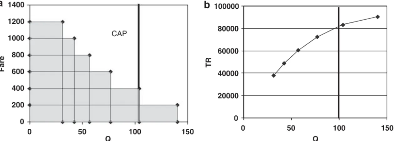
In a fully differentiated fare structure, traditional RM models assume that the demand for each fare product is independent of whether other products are available. As shown in Figure 1(a), the revenue maximizing solution is to allocate seats for all demands in decreasing fare order until capacity is reached. The seats available to the lowest fare product must be limited by capacity. The step-wise decreasing curve is the incremental revenue as function of quantity (Q). The capacity constraint is shown as the vertical line at cap¼100. Note that the data behind Figures 1 and 2 are are summarized in Table 1.
Figure 1(b) illustrates the quantitiesTRkand
Qk, denoting the total revenue and the total quantity sold given k is the lowest fare level available, as Qk ¼X k j¼1 djandTRk ¼X k j¼1 fjdj:
The total revenue increases monotonically with quantity, calculated as the area below the curve in Figure 1(a).
Now assume that the restrictions on the fare products are removed, making them fully undifferentiated (that is, ‘priceable’ demand). The only distinction between the fare products is their price levels and therefore customers will always buy the lowest fare available. Even customers willing to buy the higher fares will now buy the lowest available fare. The total revenue and the total quantity sold givenkis the
Table 1: Data for example in Figures 1 and 2
Fare product Fare Demand Fully differentiated Fully undifferentiated
fi di Qi TRi MRi TRi MRi
1 $1200 31.2 31.2 $37 486 $1200 $37 486 $1200 2 $1000 10.9 42.1 $48 415 $1000 $42 167 $ 428 3 $800 14.8 56.9 $60 217 $800 $45 536 $228 4 $600 19.9 76.8 $72 165 $600 $46 100 $28 5 $400 26.9 103.7 $82 918 $400 $41 486 $(172) 6 $200 36.3 140.0 $90 175 $200 $28 000 $(372) 0 20000 40000 60000 80000 100000 TR Q 0 200 400 600 800 1000 1200 1400 0 Q Fare 50 100 150 0 50 100 150 CAP
Figure 1: (a)Incremental revenue as function of demand (quantity). Total revenue shown as shaded area below curve. (b)Total revenue versus total demand (quantity).
lowest fare available can now be expressed as
Qk¼X
k
j¼1
djandTRk ¼fkQk:
The total revenue is shown for both the differentiated and undifferentiated case in Figure 2. With all passengers buying the lowest available fare, the total revenue for the undifferentiated case falls below that of the differentiated fare structure.
The incremental demand accommodated by opening up fare class k is dk. However the incremental revenue is notdkfk but a reduced amount, which we can calculate by accounting for the revenue lost due to buy down. The loss from buy-down is given by Qk1(fk1fk), since the aggregated demand that previously bought class k-1 now will buy class k. The incremental revenue contribution by opening up class k can therefore be written as dk
fkQk1(fk1fk). Another way to state this is that, instead of receiving the farefkby opening up class k, we obtain an adjusted fare f0k¼ [dkfkQk1(fk1fk)]/dk. The adjusted fare is also known as the marginal revenueMRkand may be calculated as the increment in total revenue per capacity unit:
MRk¼TRkTRk1
QkQk1
¼fk0
The marginal revenue is illustrated by the lower curve,MR(Q),on Figure 2(a). Note that the area below the curve corresponds to the total revenue. As more seats are made available to the lower fare, the marginal revenue becomes negative, meaning the total revenue decreases. Therefore the fare classes below $600 in this example should always remain closed.
We can therefore summarize the solution principle of the revenue optimization problem as follows: Order the fares in decreasing marginal revenue and open fares until capacity is reached or the marginal revenue becomes negative. This general principle is valid for both differentiated and undifferentiated fare structures.
GENERAL FORMULATION
In this section we develop the theory for a completely general fare structure, which may have any set of restrictions attributed to each fare product. The fare and the restrictions of a fare product determine the probability that a booking occurs for that product, which will generally depend on what other products are available as well.
An optimization strategy consists of opening up a given set of fare products, Z. Examples include opening all productsN¼{1, 2,y,n};
or keeping all products closed {}. In the previous example, we considered the subsets of opening fare products in decreasing fare -600 -400 -200 0 200 400 600 800 1000 1200 1400 a b 0 Fare Q CAP P(Q) MR(Q) 0 20000 40000 60000 80000 100000 TR Q CAP diff. un-diff. Max 50 100 150 0 50 100 150
Figure 2: (a)The demand curve P(Q) and marginal revenue MR(Q) for the undifferentiated case.(b)TR(Q) for both differentiated and undifferentiated case.
order {};{1};{1, 2},y, {1, 2,y,n}, which are
‘nested’ strategies. If we now allow a strategy to be any set of fare classes open, there will be 2n different strategies, ZDN.
The demand for a fare product depends in general on the particular optimization strategy
Z. The demand for fare productjgiven strategy
Z will be denoted dj(Z). The total demand for a given strategy is calculated as Q(Z)¼
P
jAZdj(Z). The corresponding total revenue for a given strategy (assuming no capacity constraint) is given byTR(Z)¼PjAZdj(Z)fj.
The general optimization problem can then be stated as: maxTR(Z) subject toQ(Z)pcap. The solution to the problem can most easily be solved by analyzing TR(Z) versus Q(Z) in a scatter plot where each of the 2n different strategies are plotted. These correspond to what we can call ‘pure’ strategies. In addition to the pure strategies, we may construct ‘mixed’ strategies by combining the pure strategies such that each of the pure strategies are only used for a fraction of the time.
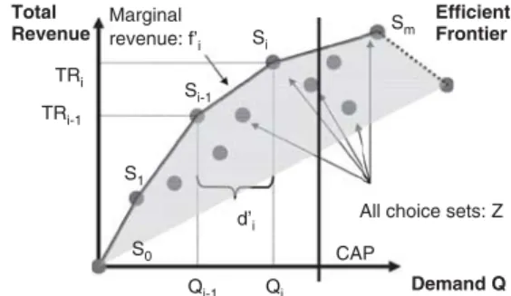
The mixed strategies trace out the convex hull of the pure strategies. This is marked in Figure 3 as the shaded area, meaning that any point within the shaded area is feasible. The solution to the optimization problem maxTR(Z) subject to Q(Z)pcap is identified as the upper boundary on the convex hull. This portion marked with the solid lines is termed the ‘efficient frontier’. Let the subset of strategies that lies on the efficient frontier (efficient sets) be denoted S0,S1,y,Sm. Here
S0¼{} is the empty set with TR(S0)¼0 and
Q(S0)¼0. The total demand and total revenue of strategy Sk is denoted by Qk and TRk respectively. Note that Figure 3 illustrates the general case where the optimal solution is obtained by a mixed strategy.
These sets are ordered according to quantity
Qk1pQk and TRk1pTRk for k¼1,y,m. The end-point for the efficient frontier is strategy
Sm, representing the maximum total revenue. The first non-empty set is in general
S1¼{1}, the highest fare in the fare structure, since it has the highest value slope, TR(Z)/
Q(Z), which is a weighted average over the fares inZ.
The marginal revenue transformation maps the original fare structure into the transformed fare structure. The demands for the transformed products are given by the marginal demandd0k while the fares of the transformed fare products are given by the marginal revenue.
d0k ¼QkQk1; k¼1;. . .;m
f0k¼ ðTRkTRk1Þ=ðQkQk1Þ; k¼1;. . .;m
The marginal demand associated with each strategy k is also called the partitioned or
incremental demand. The marginal revenues are called adjusted fares. The transformation is identical to the previous MR expression. The usefulness of the marginal revenue transforma-tion follows from the following theorem, which we have proven by direct construction of the convex hull (since the independent demand model with demand d0k and fares f0k would trace out exactly the same convex hull and are therefore equivalent).
Theorem: The marginal revenue transforma-tion transforms the original fare structure into an equivalent model with independent fare products.
Implementation of control
mechanism using fare adjustment
We have shown in the last section that the marginal revenue transformation transforms the optimization problem for an arbitrary fare
Demand Q Total Revenue Efficient Frontier S1 Si-1 Si d’i Marginal revenue: f’i TRi-1 Qi-1 Qi TRi
All choice sets: Z
S0 CAP
Sm
structure to an equivalent independent demand model. But how is the booking control nism transformed? A booking control mecha-nism in traditional RM systems calculates numerical seat availability for each booking class based on the solution of the optimi-zation problem and the current seat inventory. However, in the transformed model the strategies on the efficient frontier can involve correspond to a subset of the original booking classes, but not necessarily all classes in decreasing fare order.
Consider for example an efficient frontier with the efficient strategies {1, 2} at capacity 1, {1, 3} at capacity 2, while {1, 2, 3} is inefficient. If the capacity is 2, a nested booking limit control would protect 1 seat for {1, 2} and allow 1 booking for {1, 3}, thus the seat availability for {1, 2} would be 2 and for {1, 3} 1 correspond-ingly. It is not possible to map this to seat availability for the original classes without opening the inefficient strategy {1, 2, 3}. New distribution mechanisms would be required, where the exact number of requested seats has to be known in advance and the corresponding strategy can be shown accordingly.
Many choice models have the desirable property that the strategies on the efficient frontier are nested, SkCSl, kol, for example {1}, {1, 3}, {1, 2, 3}. Note that the nesting does not necessarily have to follow the fare order. On such nested efficient frontiers, a class once contained in an efficient strategy will also be contained in any of the next efficient strategies as capacity increases. It is therefore possible to map the original booking classes to the strategies in which they occur first with increasing capacity (or going from left to right on the efficient frontier).
When the efficient frontier is nested, the marginal revenue transformation can therefore be interpreted as the assignment of demands and fares to the original booking classes which, when fed into the optimization algorithm and the control mechanism for independent demand, produces the correct availability con-trol. This ease of implementing the control
mechanism suggests that we will in practice apply a nested approximation, even in cases where the nesting property is not exactly satisfied.
This simplification also applies to bid price control. Here, the marginal revenue going from one strategy to the next can be assigned to the newly added classes. The bid price control is therefore modified by using the marginal revenue associated with the booking class rather than the fare itself.
APPLICATIONS TO DIFFERENT
FARE STRUCTURES
In this section, we describe the application of the marginal revenue transformation and fare adjustment theory to different airline fare structures – from traditional differentiated fares to completely undifferentiated fares, along with ‘hybrid’ fare structures that include both types of fare products.
Fully differentiated fare products
Under the traditional RM assumption of fare class independence, the fare products are assumed to be adequately differentiated, such that demand for a particular fare product will only purchase that fare product. Therefore, for any set of fare products with fares fj, and demands dj, j¼1,y,n, the marginal revenue
transformation yields d0k ¼QkQk1 ¼ X j¼1;...;k dj X j¼1;...;k1 dj¼dk and f0k¼ TRkTRk1 QkQk1 ¼ P j¼1;:::;k djfj P j¼1;:::;k1 dj fj dk ¼fk
k¼1,y,n. Thus for the differentiated fare
product case, the marginal revenue transforma-tion acts as an identity and both demands and fares are unaffected. We can refer to this
demand as being ‘product-oriented’. Let us denote the unadjusted fare byf0kprod.
Completely undifferentiated fare products
We now apply the marginal revenue transfor-mation to a single flight leg with a fully undifferentiated fare structure, again assuming deterministic demand. The definitions of fares
fj, and demands dj, j¼1,y,n are unchanged.
Due to the fully undifferentiated fare structure, passengers will only buy the lowest available fare. Let k be the lowest open fare product, then the demand for all other fare pro-ducts becomes zero, dj¼0 for jakHence the cumulative demand equals the demand for the lowest open fare product dk¼Qk, k¼1,y,n. The demand Qk¼Qnpsupk (assuming fk is the lowest open) can be expressed as a sell-up probability psupk from n-k, times a base demandQnfor the lowest class n.
The marginal revenue transformation deter-mines the adjusted fares. The demand is calculated as d0k¼QkQk1¼dkdk1
¼Qn(psupkpsupk1).
The adjusted fares are given by
fk0¼TRkTRk1 QkQk1 ¼fkQkfk1Qk1 QkQk1 ¼ fkpsupkfk1psupk1 psupkpsupk1 : Let us denote this by f0kprice.
Note that the highest fare value is un-adjusted: f10 ¼TR1TR0 Q1Q0 ¼f1d10 d10 ¼f1
Consider the special case of exponential sell-up Qk¼Qnpsupk¼Qnexp(b( fkfn)) and assume for simplicity an equally spaced fare-grid with fk1fk¼D. The marginal revenue transformation yields:
dk0 ¼QnexpðbfnÞ
ðexpðbfkÞ expðbfk1ÞÞ:
fk0 ¼fkfM; where
fM ¼D expðbDÞ
1expðbDÞ
The adjusted fare can therefore be expressed a the original fare minus a positive constant called the fare modifier, fM. For a general fare structure, the fare modifier will differ by class. Because the fare modifier is the cost associated with buy-down, it is also termed the price elasticity cost.
In Table 1, the constant fare modifier can be seen fM¼$572. Since seats are only allocated to fare classes with positive adjusted fares, we can interpret fM as the lowest open fare. In the limit D-0, using l’Hopital’s rule we obtain fM-1/b for D-0, which depends only on the beta parameter in the exponential demand model.
Hybrid demand in mixed fare structures
In this section we show how to optimize a single leg with a fare structure consisting of a mix of differentiated and undifferentiated fare products assuming deterministic demand, using the marginal revenue transformation. This is the so-called hybrid demand case. The fare class demands are decomposed into contributions from both differentiated (pro-duct-oriented) and un-differentiated (price-oriented) demand:
dj ¼djprodþd price
j ; j¼1;. . .; n
The marginal revenue transformation deter-mines the adjusted fares. The demand for each fare class is obtained as
dk0 ¼QkQk1¼ X j¼1;...;k djprodþdkprice ! X j¼1;...;k1 djprodþdkprice1 !
¼dkprodþQnðpsupkpsupk1Þ Definerk¼dkprod/(dkprodþQn(psupkpsupk1)) as the ratio of product demand to total demand.
The adjusted fare is given by fk0 ¼TRkTRk1 QkQk1 ¼ P j¼1;:::;k djprodfjþd price k fk ! P j¼1;:::;k1 djprodfjþd price k1fk1 !
dkprodþQnðpsupkpsupk1Þ
¼d
prod
k fkþQnðfkpsupkfk1psupk1Þ
dkprodþQnðpsupkpsupk1Þ
¼rkf0 prod
k þ ð1rkÞf0 price
k :
Thus the adjusted fare in the hybrid case is calculated by a demand-weighted average of the unadjusted fare used for the product-oriented demand and the adjusted fare for the price-oriented demand.
EXTENSIONS TO STOCHASTIC
MODELS
In the previous sections, we considered deter-ministic models on a single flight leg, in order to present the theory more clearly. In this section, we show that the marginal revenue transformation also holds for stochastic models. Furthermore, it extends to network optimiza-tion provided the choice probabilities for the different O-D paths are independent.
Talluri and van Ryzin (1998) provided a consistent formulation of a stochastic network dynamic programming model, but it cannot be implemented in practice because of the curse of dimensionality. In practice, stochastic network optimization methods for airline revenue management typically require some heuristic aspects to generate approximate solutions. Therefore, if we show that the marginal revenue transformation holds exactly for the DP approach, we can argue that it can also be applied to any other solution method. We start with the one leg model first, followed by a straightforward generalization to the network problem with independent O-D paths.
DP formulation for a discrete choice model of demand
The dynamic program for one leg with an arbitrary fare structure, such that demand behaviour is modelled by a discrete choice model, was developed by Talluri and van Ryzin (2004). Dynamic programming models assume that the bookings can be modelled as a Markov process with small time steps such that the probability of more than one booking is negligible. The arrival probability of a book-ing is denoted by ltX0 and the remaining capacity xt for each t serves as state variable. At the beginning of each time interval, the airline can choose the set of products available for sale. A strategy therefore consists of the set of open classes Zt(x)DN, where N is the set of all classes.
Given an arrival and strategy Zt, the prob-ability that productjAZtis chosen is denoted by
pj(Zt). The expected demand for product j in time slicet is thereforedj(Zt)¼lpj(Zt), which is the probabilistic analogy of the deterministic models of the sections ‘General formulation’ and ‘Applications to different fare structures’. The DP model can handle time dependent choice probabilities and arrival rates as well, but for the sake of simplicity, we did not introducet
indices for the choice probabilities and the arrival rate.
The probability that a booking occurs for any product, given an arrival and choice setZ, is therefore
QðZÞ ¼X
j2Z pjðZÞ
and the corresponding expected total revenue is
TRðZÞ ¼X
j2Z
pjðZÞ fj
Bellman equation
The dynamic program proceeds by considering the concept of expected optimal future reven-ue, or revenue to go,Jt(x). The goal is to find
the strategy which maximizes J0(cap), the optimal revenue at the beginning of the booking process. The Bellman equation for our problem now states that the optimal future revenue satisfies the recursion relation:
Jt1ðxÞ ¼max
ZNflðTRðZÞ þQðZÞ Jtðx1ÞÞ
þð1lQðZÞÞ JtðxÞg;
with boundary conditions JT(x)¼Jt(0)¼0. The first term in the above corresponds to the case when a sell occurs; the airline receives one booking from the set of open classes in Z, and continues with one seat less. The second term corresponds to the no-sell situation, where the airline continues with the same amount of seats. The above optimization problem has to be solved for each x and t in order to find the optimal strategy Z. Introdu-cing the bid-price vector
BPtðxÞ ¼JtðxÞ Jtðx1Þ
one can write the optimization problem as:
Jt1ðxÞ ¼ JtðxÞ þ lmax
ZNðTRðZÞ
BPtðxÞ QðZÞÞ
ð1Þ
Observe now that for allxandt, this problem is of the same form, namely
max
ZNðTRðZÞ BPQðZÞÞ ð2Þ
where only the value of the bid-price may change.
Efficient frontier
The problem of optimizingmax
ZNðTRðZÞ BP QðZÞÞ is most easily analyzed by drawing
TR(Z) versus Q(Z) in a scatter plot for all possible strategies of open classes, together with the straight lineBPQfor specific values of the bid-price. For comparison, the plot in Figure 4 is identical to Figure 3 describing the efficient frontier for the deterministic case.
The optimum for the specific BP in the chart is attained where the parallel shifted lineBPQis tangent to the convex hull of the
points (Q(Z),TR(Z)). This strategy is marked as Siin the chart.
Since the bid-price is always positive, only strategies which lie on the efficient frontier from S0 to Sm the set with maximal total revenue can be solutions to the problem. We refer to the discussion regarding the efficient strategies from the deterministic case, which translates identically to the DP case.
Marginal revenue transformation
The optimal strategy as function of the bid-price can only consist of one of the vertices on the efficient frontier. As long as the bid-price is higher than the highest fare, we should close all classes.1 We denote this strategy by S0. If the bid-price falls below f1 the optimal strategy is initially S1, until the bid-price falls below the slope of the convex hull betweenS1toS2. The slopes of the efficient frontier correspond to the critical values of the bid-price, where the optimal strategy changes. The optimal strategy for a given bid price BP is found by walking along the efficient frontier from one strategy to the next, increasing sales volume, as long as
MRk ¼TRðSkÞ TRðSk1Þ
QðSkÞ QðSk1Þ
XBP:
The last strategy obtained this way is the optimal strategy of open booking classes for bid priceBP. Once the efficient frontier is known, the bid-prices can be calculated from the DP formulation recursively. Because the efficient frontier contains only a few of the possible
Demand Q Total Revenue Efficient Frontier S1 Si-1 Si TRi-1 TRi Qi-1 Qi S0 Sm max BP*Q p’i Marginal revenue: f’i
strategies, there are potentially many fare structures with corresponding choice models (identified by a set ofpj(Z)) which will lead to the same efficient frontier. All these models will have the same bid-price. In particular consider the independent demand model defined by:
pk0 ¼QðSkÞ QðSk1Þ; k¼1;. . .;m:
fk0 ¼MRk
¼TRðSkÞ TRðSk1Þ
QðSkÞ QðSk1Þ
; k¼1; ;m
This is identical to the marginal revenue transformation introduced in the section ‘Gen-eral formulation’. Using the transformed choice model (primed demand and fares) in an independent demand DP instead of the original choice model DP, the Bellman equa-tion will produce the same bid-prices. Further-more, as explained in the section ‘General formulation’, we can associate the marginal revenue or adjusted faresf0kto the newly added classes inSk\Sk1provided the efficient frontier is nested.
Network DP formulation
for a discrete choice model of demand
Let us also touch briefly on the network DP formulation of Talluri and van Ryzin (1998), generalized to independent discrete choice models for each itinerary. In each time slice there is at most one request for the whole network and the rate l is the probability that the request is for a given itinerary. The state becomes a vector (x1,?,xL) of the remaining capacities for each leg. The second term on the right hand side of equation (1) above becomes a sum over all itineraries, where the bid-price for an itinerary is the difference in expected future revenue if on each leg one seat is removed. An optimal strategy for each itinerary has to be chosen. The optimization problem therefore decomposes into a set of
independent optimizations of the form (2) for each itinerary.
The DP network model has no practical importance, since the number of possible states explodes with capL. However the marginal revenue transformation holds as well. This leads us to conclude that any heuristic network algorithm which assumes independent demand by O-D itinerary can be easily extended to deal with arbitrary fare structures by applying the marginal revenue transformation. This will be illustrated in the example with DAVN-MR below.
Recover pricing DP model as a special case
Let us consider as an example the case of a fully undifferentiated fare structure. This model is nested by fare order and we can there-fore identify the efficient strategy index with the original booking class index. A strategy
Sk therefore has class k and all classes with higher fares open. If we insert the trans-formed demand and transformed fares into the Bellman recursion formula for a DP with independent demand, we obtain the following problem. max S X i2S pi0ðfi0BPÞ ¼max k Xk i¼1 QðSiÞ QðSi1Þ ð Þ
TRðSiÞ TRðSi1Þ QðSiÞ QðSi1Þ BP ¼max k ½QðSkÞðfkBPÞIn the last equation we have used that we have a telescopic sum and that all demand resides in the lowest open class and thus
TR(Sk)¼fkQ(Sk). The last expression is iden-tical to the pricing DP model of Gallego and Van Ryzin (1997). The first optimization problem above for independent demand is
easily solved since only classes where f0kXBP should be included in the strategy S. If we further insert the exponential sell-up with equally spaced fares we obtain
max S X i2S pi0ðfi0 BPÞ ¼max k ½expðb ðfkfnÞÞ ðfkBPÞ
We have shown in the section ‘Applications to different fare structures’ that the fare modifier for exponential sell-up and equally spaced fare grid is a constant. Thus the open classes are exactly those which have fifMXBP, a result which would not be immediately clear from optimization problem on the right hand side.
Leg RM: EMSRb-MR
Here we show how EMSRb can be extended to optimize a general fare structure. First we will briefly consider the results for standard unadjusted EMSRb, in order to be able to compare with the transformed EMSRb-MR. In standard EMSRb we consider independent fare products with fares fi, with normally distributed demandsdiBN(mi,si2),i¼1,y,n. The aggregated demand for fare product
i¼1,y,k is also normally distributed with
average m1,k¼ P i¼1 k m i, variance s1,2k¼ P i¼1 k s i 2
and average faref1;k ¼m1;1k Pk
i¼1mifi.
The joint protection levelpkis then given by pk ¼m1;kþs1;kF1ð1fkþ1=f1;kÞ, and the
booking limit byBLk¼cappk.
For a general fare structure we need to apply the formalism presented in the previous sections, which consists of the following steps:
(1) Determine the strategies k¼1,y,m on
the efficient frontier.
(2) Apply the marginal revenue transformation to both demands and fares.
(3) Apply EMSRb in the normal fashion using the transformed demands and fares.
This method, called EMSRb-MR, thus considers independent normally distributed demands d0kBN(mk,sk2), with fares f0k, k¼1,
y,m. Note that the demands are related to the
strategies not the individual fare products. The aggregated demand, variance, and average fares are calculated analogously using the trans-formed demands and fares and hence the formulas for the joint protection level and the booking limit become exactly the same: pk0 ¼m1;kþs1;kF1ð1f 0 kþ1=f 0 1;kÞ, and BL0k¼capp0k.
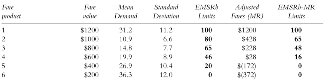
Consider again the case of fully undiffer-entiated fare products with equal spaced fares, as presented in Table 1 and in section ‘Applications to different fare structures’. In this case the strategies become nested and we may associate an adjusted fare with each strategy. For simplicity (and ease of compar-ison) we will assume that the demands and standard deviations are identical to those of the fully differentiated case.
Table 2 compares the standard EMSRb results in the case of differentiated fares with
Table 2: Comparison of Standard EMSRb and EMSRb-MR Booking Limits
Fare product Fare value Mean Demand Standard Deviation EMSRb Limits Adjusted Fares (MR) EMSRb-MR Limits 1 $1200 31.2 11.2 100 $1200 100 2 $1000 10.9 6.6 80 $428 65 3 $800 14.8 7.7 65 $228 48 4 $600 19.9 8.9 46 $28 16 5 $400 26.9 10.4 20 $(172) 0 6 $200 36.3 12.0 0 $(372) 0
the modified booking limits coming from the EMSRb-MR approach in the case of undiffer-entiated fares. Note that the adjusted fares used as input to EMSRb after the marginal revenue transformation lead to closure of the lowest two classes with negative marginal revenues. Classes 2 through 4 also get reduced seat availability, given that the estimated potential for sell-up has been incorporated into the marginal revenue values of each class.
The adjusted EMSRb-MR overcomes spiral down by modifying the resulting booking limits to account for the estimated sell-up potential, and thereby the dependent demand forecasts, which results in closing availability to the inefficient fare products (that is with negative adjusted fares).
Network RM: DAVN-MR with differentiated and undifferentiated fare structures
For a large network airline, it is common to offer a variety of fare structures in different O-D markets, each with different restrictions, as required to respond to competitors in each market. However, individual flight legs to or from a connecting hub provide seats to multiple O-D markets, each of which can have different fare structures. In this section we show how to optimize a network with a mix of differentiated fare products and undifferenti-ated fare products. As an example we will use DAVN (Displacement Adjusted Virtual Nesting).
The marginal revenue transformation ap-plied to DAVN (termed DAVN-MR) results in transforming both demands and fares as described in the previous sections. A particu-larly simple expression for the adjusted fare is obtained by assuming exponential sell-up and equally spaced fares, as shown previously. The adjusted fare becomes
adj f ¼f0XDC ¼f fMXDC:
Here PDC refers to the standard DAVN approach of calculating the marginal network
revenue contribution of accepting an O&D passenger by subtracting the displacement costs of carrying a passenger on connecting legs. Further, we have used the previous result that the adjusted fare can be expressed as the fare minus a fare modifier. Thus this formula extends the standard DAVN formula by just an additional term ‘fM’. Note thatfM¼0 for differentiated fare products. The undifferen-tiated fare products are mapped to lower buckets since fM>0 (except the highest un-differentiated fare class). Also note that all undifferentiated fare products with fares fofM will be closed (regardless of remaining capacity) since they map to negative adjusted fares. DAVN-MR is then applied by running DAVN in the standard fashion on the transformed fare structure to produce booking limits by bucket (in marginal revenue scale) for each leg. Finally, note that the formula for the adjusted fare is valid for an arbitrary fare structure with nested efficient frontier, but there the fare modifier will vary by class.
SIMULATION RESULTS USING
PODS
In this section, we present simulation results from PODS (Passenger Origin Destination Simulator) to illustrate the revenue impacts of applying the marginal revenue transformation in DAVN-MR, as described above. PODS and its various components have been widely
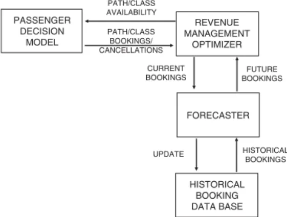
PASSENGER DECISION MODEL REVENUE MANAGEMENT OPTIMIZER FORECASTER HISTORICAL BOOKING DATA BASE CURRENT BOOKINGS HISTORICAL BOOKINGS FUTURE BOOKINGS PATH/CLASS AVAILABILITY PATH/CLASS BOOKINGS/ CANCELLATIONS UPDATE
described in the literature – see for example, Hopperstad (1997), Belobaba and Wilson (1997), Lee (1998), and Carrier (2003). The central concept in PODS is that the models of the revenue management systems and the model of passenger choice are contiguous but independent. That is, the revenue management system(s) define the availability of path/classes in a market and the generated passengers pick from the available path/classes and book. The only information available to the revenue management system(s) of the simulated airlines for setting path/class availability is the history of (previously simulated) passenger bookings. Figure 5 illustrates this basic architecture.
In PODS, each simulated passenger chooses among available path/class alternatives (that is, itinerary and fare product combinations) with fares lower than that passenger’s randomly drawn maximum willingness-to-pay (WTP). Business passengers have a higher input mean WTP than leisure travellers. If there exist more than one available path/class meeting this WTP criterion, the passenger then chooses the alternative with the lowest generalized cost, defined as the sum of the actual fare and the disutility costs with the restrictions (if any) associated with each fare class. A passenger will ‘sell up’ from a preferred lower fare class (with a lower generalized cost) to a more expensive
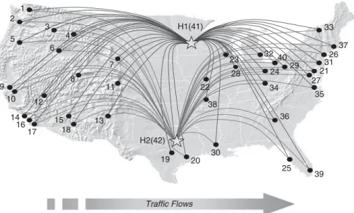
H1(41) 19 28 H2(42) 4 3 2 1 10 9 8 7 6 5 15 17 16 14 12 11 22 21 20 18 27 26 25 24 23 33 32 31 30 29 39 38 37 36 35 34 40 13 Traffic Flows
Figure 6:PODS network D.
NO NO NO 0 6 NO NO NO 0 5 NO NO NO 0 4 NO NO NO 0 3 NO NO NO 0 2 NO NO NO 0 1 Non Refund Cancel Fee Min Stay AP FARE CLASS SEMI-DIFFERENTIATED UNDIFFERENTIATED YES YES NO 0 6 YES YES NO 0 5 YES YES NO 0 4 YES YES NO 0 3 NO YES NO 0 2 NO NO NO 0 1 Non Refund Cancel Fee Min Stay AP FARE CLASS
one, therefore, if the lower class is closed due to RM controls and if the higher fare is still lower than the passenger’s WTP. The simulated sell-up behaviour is thus imbedded in the PODS passenger decision model, rather than specified as an input sell-up parameter.
Figure 6 shows the geometry of network D, one of the standard PODS networks. In net-work D there are two airlines, each with their own hubs. The traffic flow is from the 20 western cities to the hubs and to the 20 eastern cities. Both airlines employ three connecting banks per day, resulting in each airline operat-ing 126 legs, which produce 1446 paths in 482 markets.
Six fare classes are assumed, and simulation results are provided here for both an undi-fferentiated and a semi-diundi-fferentiated fare structure, as shown in Figure 7. In the undi-fferentiated case there are no fare restrictions or advance purchase rules. In the semi-differen-tiated case, two restrictions (no refunds in case
of cancellation and a fee for changing reserva-tions) are applied to lower fare classes (Figure 7). The focus of the simulation study is on Airline 1 and its use of hybrid forecasting and DAVN-MR. In the simulations, the effects of each of the two components of the transforma-tion were studied separately. Three scenarios were considered:
K Standard: Airline 1 uses standard path/fare class forecasting with DAVN (baseline). K Hybrid: Airline 1 changes to Q/hybrid
forecasting,withoutfare adjustment.
K DAVN-MR: Airline 1 adds fare adjustment to its Q/hybrid forecasting.
Note that hybrid forecasting for the fully undifferentiated fare structure corresponds to only using the price-oriented forecasting model (so-called Q-forecasting) [Belobaba and Hopperstad (2004)].
The three scenarios are examined, for the undifferentiated and the semi-differentiated
100.0 115.8 134.5 0 25 50 75 100 125 150 Standard Revenue Index
Monopoly: Un-differentiated fare-structure
108.7 117.5 135.9 0 25 50 75 100 125 150 Revenue Index
Monopoly: Semi-differentiated fare-structure
85.4 85.1 74.1 0 20 40 60 80 100 Load Factor
Monopoly: Un-differentiated fare-structure
85.3 85.1 72.3 0 20 40 60 80 100 Load Factor
Monopoly: Semi-differentiated fare-structure DAVN-MR
Hybrid
Standard Hybrid DAVN-MR
Standard Hybrid DAVN-MR
Standard Hybrid DAVN-MR
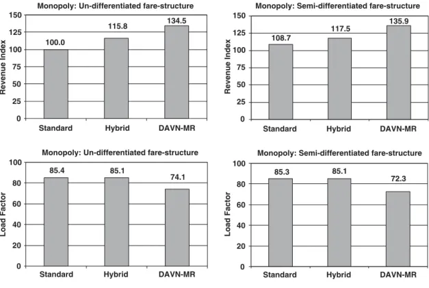
Figure 8: Simulation results for the monopoly case with undifferentiated and semi-differentiated fare-structures in network D.
fare structures, first in a monopoly environment where only Airline 1 is present and then in a competitive environment where the second airline uses standard path/fare class forecasting and traditional DAVN network RM optimization.
Monopoly case
The simulation results are presented in Figure 8. In the panels the revenue index and load factor (LF) are shown both for the undifferentiated and the semi-differentiated fare structures. The revenue index is reported relative to the baseline monopoly case in which the airline employs standard forecasting and optimization.
The results show that applying hybrid forecasting only, for both fare structures, leads to significant revenue gains on the order of 10 per cent–16 per cent. The reason is that hybrid forecasting considers the buy-down
potential of the price oriented demand and reduces spiral down. Note that load factors for standard and hybrid forecasting are almost identical. Hybrid forecasting can be thought of as an attempt to ‘re-map’ passengers that bought down back to their original fare class.
Applying fare adjustment by moving to full DAVN-MR leads to a further revenue increase of about 16 per cent in both cases. The revenue benefit of applying fare adjustment is significant since its effect is to close lower fare classes, which further restricts buy-down. This effect can clearly be seen from the load factors. Applying fare-adjustment leads to a significant drop in load factor from 85 per cent to 72 per cent–74 per cent.
Competitive case
The simulation results for the two-airline competitive case are presented in Figure 9,
100.0 110.0 120.3 100.0 102.0 114.0 0 25 50 75 100 125 150 Standard Revenue Index
Competition: Un-differentiated fare-structure
AL1 AL2 AL1 AL2
AL1 AL2 AL1 AL2 99.7 112.9 128.9 99.7 101.9 112.9 0 25 50 75 100 125 150 Revenue Index
Competition: Semi-differentiated fare-structure
85.5 84.8 68.5 84.4 85.5 93.1 0 25 50 75 100 Load Factor
Competition: Un-differentiated fare-structure
85.5 84.6 64.6 84.4 85.7 93.8 0 25 50 75 100 Load Factor
Competition: Semi-differentiated fare-structure DAVN-MR
Hybrid
Standard Hybrid DAVN-MR Standard Hybrid DAVN-MR
Standard Hybrid DAVN-MR
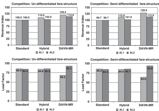
Figure 9: Simulation results in the competitive case with undifferentiated and semi-differentiated fare-structures in network D.
with the panels organized as in Figure 8. The revenue index is reported relative to a baseline scenario in which both airlines employ standard forecasting and DAVN network RM controls. In a competitive simulation environment, the results show that applying hybrid forecast-ing again leads to significant revenue gains on the order of 10 per cent–13 per cent. In contrast to the monopoly case, the revenue index for standard forecasting is nearly the same for the unrestricted and semi-restricted cases. The reason for this is that in a competitive environment spiral-down is magnified by competitive feedback, as passengers have a greater set of path/class alternatives from which to choose. With more alternatives, the lowest class 6 is more frequently available on one of the airlines. The consequence of this avail-ability is that passengers who might have bought-up to class 1 or 2 (from, say, classes 3 or 4) do not, because the fare difference between these classes and class 6 is mostly greater than the disutility the passengers attribute to the restrictions. Quite simply, the sell-up potential in a competitive market is lower than in the monopoly case, even with the same passenger choice characteristics.
Applying fare adjustment and thus full DAVN-MR gives a further 9 per cent–14 per cent revenue increase. The use of DAVN-MR by Airline 1 causes load factors to drop from 85 per cent to 65–68 per cent. The competitor picks up the spill-in of low fare passengers rejected by Airline 1 and obtains load factors of 93 per cent–94 per cent. Note that app-lying DAVN-MR is not a zero-sum game. When Airline 1 moves to DAVN-MR, Airline 2 also benefits from Airline 1’s change in RM control. Airline 1’s gain comes from extracting higher yields from passengers willing to buy up to higher fare classes. The result is a drop in Airline 1’s load factor (from 86 per cent to 65 per cent) with a consequent 10–20 per cent increase in the apparent demand for Airline 2, which gives it a revenue increase due to higher load factors, albeit at much lower yields.
CONCLUSION
We have described an approach to transform the fares and the demand of a general discrete choice model to an equivalent independent demand model. This transformation is of great practical importance to airlines, as it allows the continued use of the optimization algorithms and control mechanisms of traditional revenue management systems, developed more than two decades ago under the assumption of independent demands for fare classes. The transformation and resulting fare adjustment approach is valid for both static and dynamic optimization and extends unchanged to the case of network problems (provided the net-work problem is separable into independent path choice probability). Assuming the efficient frontier is nested (or approximately nested), the implementation of the control mechanism can be implemented very elegantly by associating to each class the corresponding adjusted fare obtained from the marginal revenue transfor-mation and then applying the control mechan-ism in the standard way.
NOTE
1 While this cannot be possible in our simple stationary one-leg world, it could happen for the network problem, or when the fare structure would depend on the time step.
REFERENCES
Barnhart, C., Belobaba, P. P. and Odoni, A. R. (2003) Applications of operations research in the air transport industry.Transportation Science37(4): 368–391.
Belobaba, P. P. (1987) Air travel demand and airline seat inventory management. Unpublished Ph.D. Thesis, Massachusetts Institute of Technology, Cambridge, MA. Belobaba, P. P. (1989) Application of a probabilistic decision
model to airline seat inventory control.Operations Research37: 183–197.
Belobaba, P. P. (1992)Optimal vs. Heuristic Methods for Nested Seat Allocation, Proceedings of the AGIFORS Reservations and Yield Management Study Group, Brussels.
Belobaba, P. P. (1998) The evolution of airline yield manage-ment: Fare class to origin-destination seat inventory control. In: D. Jenkins (ed.)The Handbook of Airline Marketing. New
York, NY: The Aviation Weekly Group of the McGraw-Hill Companies, pp. 285–302.
Belobaba, P. and Hopperstad, C. (2004) Algorithms for revenue management in unrestricted fare markets. Presented at the Meeting of the INFORMS Section on Revenue Manage-ment, Massachusetts Institute of Technology, Cambridge, MA.
Belobaba, P. P. and Weatherford, L. R. (1996) Comparing decision rules that incorporate customer diversion in perish-able asset revenue management situations. Decision Sciences
27(2): 343–363.
Belobaba, P. P. and Wilson, J. L. (1997) Impacts of yield management in competitive airline markets. Journal of Air Transport Management3(1): 3–10.
Boyd, E. A. and Kallesen, R. (2004) The science of revenue management when passengers purchase the lowest available fare.Journal of Revenue and Pricing Management3(2): 171–177. Bratu, S. J-C. (1998) Network value concept in airline revenue management. Master’s thesis, Massachusetts Institute of Technology, Cambridge, MA.
Brumelle, S. L. and McGill, J. I. (1993) Airline seat allocation with multiple nested fare classes. Operations Research 41: 127–137.
Carrier, E. J. (2003) Modeling airline passenger choice: Passenger preference for schedule in the passenger origin-destination simulator. Unpublished Master’s Thesis, Massachusetts Institute of Technology, Cambridge, MA.
Cooper, W. L., Homem-de-Mello, T. and Kleywegt, A. J. (2006) Models of the spiral-down effect in revenue management.
Operations Research54(5): 968–987.
Curry, R. E. (1990) Optimal airline seat allocation with fare classes nested by origin and destinations.Transportation Science
24(3): 193–204.
Fiig, T., Isler, K., Hopperstad, C. and Cleaz-Savoyen, R. (2005) DAVN-MR: A Unified Theory of O&D Optimization in a Mixed Network with Restricted and Unrestricted Fare Products.AGIFORS Reservations and Yield Management Study Group Meeting,Cape Town, South Africa, May.
Gallego, G. and van Ryzin, G. (1997) A product, multi-resource pricing problem and its application to network yield management.Operations Research45: 24–41.
Guo, J. C. (2008) Estimation of sell-up potential in airline revenue management systems. Unpublished Master’s Thesis, Massachusetts Institute of Technology, Cambridge, MA. Hopperstad, C. H. (1997) PODS Modeling Update.AGIFORS
Yield Management Study Group Meeting,Montreal, Canada. Hopperstad, C. H. (2007) Methods for Estimating Sell-Up.
AGIFORS Yield Management Study Group Meeting, Jeju Island, Korea.
Isler, K., Imhof, H. and Reifenberg, M. (2005) From Seamless Availability to Seamless Quote. AGIFORS Reservations and
Yield Management Study Group Meeting, Cape Town, South Africa, May.
Lautenbacher, C. J. and Stidham, S. J. (1999) The underlying markov decision process in the single-leg airline yield management problem.Transportation Science33: 136–146. Lee, A. Y. (1998) Investigation of competitive impacts of
origin-destination control using PODS. Unpublished Master’s Thesis, Massachusetts Institute of Technology, Cambridge, MA.
Lee, T. C. and Hirsch, M. (1993) A model for dynamic airline seat inventory control with multiple seat bookings. Transporta-tion Science27: 252–265.
Littlewood, K. (1972)Forecasting and Control of Passenger Bookings, 12thAGIFORS Annual Symposium Proceedings, Nathanya, Israel, pp. 95–117.
McGill, J. I. and van Ryzin, G. J. (1999) Revenue management: Research overviews and prospects.Transportation Science33(2): 233–256.
Saranathan, K., Peters, K. and Towns, M. (1999) Revenue Management at United Airlines.AGIFORS Reservations and Yield Management Study Group, April 28, London.
Simpson, R. W. (1989) Using network flow techniques to find shadow prices for market and seat inventory control, memorandum M89-1, MIT Flight Transportation Laboratory. Cambridge, MA: Massachusetts Institute of Technology. Smith, B. C., Leimkuhler, J. F. and Darrow, R. M. (1992)
Yield management at american airlines. Interfaces 22(1): 8–31.
Smith, B. C. and Penn, C. W. (1988) Analysis of alternative origin-destination control strategies. AGIFORS Symposium Proceedings28: 123–144.
Talluri, K. T. and van Ryzin, G. (1998) An analysis of bid-price controls for network revenue management. Management Science44: 1577–1593.
Talluri, K. T. and van Ryzin, G. (2004) Revenue management under a general discrete choice model of consumer behavior.
Management Science50(1): 15–33.
Tretheway, M. W. (2004) Distortions of airline revenues: Why the network airline business model is broken.Journal of Air Transport Management10(1): 3–14.
Vinod, B. (1995) Origin and destination yield management. In: D. Jenkins (ed.)The Handbook of Airline Economics. New York, NY: The Aviation Weekly Group of the McGraw-Hill Companies, pp. 459–468.
Williamson, E. L. (1992) Airline network seat inventory control: methodologies and revenue impacts. Ph.D. Thesis, Massachusetts Institute of Technology, Cambridge, MA.
Wollmer, R. D. (1992) An airline seat management model for a single leg route when lower fare classes book first.Operations Research40(1): 26–37.