Methods in Economic Farm Modelling

(1)

Institut für Lebensmittel- und Ressourcenökonomik der Rheinischen Friedrich-Wilhelms-Universität zu Bonn

Methods in Economic Farm Modelling

I n a u g u r a l - D i s s e r t a t i o n

zur

Erlangung des Grades

Doktor der Agrarwissenschaften (Dr.agr.)

der

Hohen Landwirtschaftlichen Fakultät der

Rheinischen Friedrich-Wilhelms-Universität zu Bonn

vorgelegt am 22. September 2009 von Alexander Gocht

(2)

Referent: Prof. Dr. Thomas Heckelei

Korreferent: Prof. Dr. Ernst Berg

Tag der mündlichen Prüfung: Freitag 11. Dezember, 2009

(3)

(4)

(5)

Acknowledgements

First, I would like to express my sincere gratitude to Prof. Thomas Heckelei, who has been an excellent supervisor and gave me the opportunity to work at the Institute of Food and Resource Economics (ILR) in Bonn from 2006 to 2008. In particular, Chapter 4 and Chapter 5 were developed with his close cooperation. I am very grateful for his encouragement and the way he helped me to take a broader perspective on economic problems. Furthermore, I very much appreciate Prof. Ernst Berg’s evaluation of this thesis. Within our CAPRI working group at ILR, Dr. Wolfgang Britz supported this thesis by spurring inspirational discussions. The research in Chapter 5 is a joint effort, and I learned much from him, not only from his knowledge of economic modelling, but also from his brilliant programming skills. I would also like to thank everyone at the ILR for a very pleasant and inspiring atmosphere - in particular, Hans Josef Greuel for his IT support. Part of this thesis was developed at the Johann Heinrich von Thünen-Institute (vTI) in Braunschweig before I moved to Bonn. The research presented in Chapter 2 was conducted at this time in close cooperation with Kelvin Balcombe from Reading University (UK). I am very grateful for his help and advice. I also would like to thank two anonymous referees from Agricultural Economics whose comments substantially formed and improved the work in Chapter 2. I would like to convey my thanks to Dr. Jeroen Buysse, who provided the data for the application of the methods developed in Chapter 4. The work in Chapter 5 could not have been accomplished without the help of Pol Marquer from Eurostat. He extracted several data selections for the presented farm type layer in Chapter 5. Furthermore, I would like to thank my colleagues at vTI - namely Dr. Werner Kleinhanß and Dr. Frank Offermann, who commented on Chapter 3. In addition to direct professional support, many people have helped me during the last few years. I would like to express my sincere thanks to Prof. Heinrich Becker and Prof. Thoralf Münch for their friendship and assistance. Many thanks also to Dr. Hiltrud Nieberg and Dr. Adriana Cristoiu for their help and advice. I would also like to thank my family, as this work would not have been possible without advice and support from all of you. Finally, I dearly thank Claudia for her love and support, which made this entire endeavour worthwhile, and my daughter Rosa, for being an inspiration in my life.

(6)

(7)

Kurzfassung

Methoden zur ökonomischen Modellierung landwirtschaftlicher

Betriebe

Die Arbeit untersucht und entwickelt Methoden zur Bewertung von landwirtschaftlichen Betrieben im Rahmen der Effizienzanalyse und zur Abschätzung von Anpassungsreaktionen induziert durch die Veränderung von politischen und wirtschaftlichen Rahmenbedingungen. Die Dissertation ist in vier Hauptkapitel gegliedert.

Im Kapitel 2 wird die Methodik der Effizienzanalyse, bekannt unter dem Namen Data Envelopment Analysis (DEA) um den Ansatz zur Ableitung von Konfidenzintervallen erweitert, um die Aussagekraft der Effizienzmaße zu überprüfen. Die Bewertung und der Vergleich von landwirtschaftlichen Betrieben mit DEA sind in der Literatur häufig zu finden. Dabei werden die Ursachen von Ineffizienz oft mittels einer anschließenden Regressionsanalyse ermittelt. Die abgeleiteten Konfidenzintervalle zeigen jedoch deutlich, dass ohne Berücksichtigung der stochastischen Natur der Effizienzmaße kaum aussagekräftige Schluss-folgerungen über die wahre Natur von Ineffizienzen gegeben werden können.

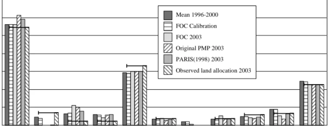
Im Kapitel 3 wird das Simulationsverhalten von mathematischen Program-mierungsmodellen (MP) induziert durch die Veränderung von politischen und wirtschaftlichen Rahmenbedingungen untersucht. Im Gegensatz zur Anwendung auf einzelbetrieblicher Ebene, wo eine Spezifizierung des Modells durch vergleichweise viele Informationen erfolgen kann, sind Analysen zur Politikfolgenabschätzung häufig nur sinnvoll, wenn diese auf repräsentativen Betriebsgruppen basieren und damit aggregierte Effekte quantifiziert werden können. Zur Spezifizierung der entsprechenden Modelle stehen jedoch oftmals nur wenige Informationen zur Verfügung. Weiterhin besteht das Problem, dass wichtige Entscheidungsvariablen den beobachteten Werten entsprechen sollten, was als Kalibrierung des MP-Modells bezeichnet wird. Um dennoch MP-Modelle für repräsentative Politikfolgen-abschätzung auf Betriebsebene nutzen zu können, sind positiv-mathematische Programmierungsmodelle (PMP), die mittels einer nicht-linearen Komponente der Zielfunktion das Model kalibrieren und das Simulationsverhalten mitbestimmen, entwickelt worden. Der Einfluss verschiedener vorgeschlagener PMP Methoden auf das Simulationsergebnis werden mit dem Betriebsgruppenmodel FARMIS quantifiziert und ex post mit beobachteten Werten verglichen. Dafür werden 45 Betriebsgruppen benutzt. Auf diese Betriebsgruppenmodelle werden die PMP-Kalibrierungsmethoden für das Jahr 1996/97 angewendet und beobachtete Deckungsbeiträge aus dem Jahr 2002/03 als Schock implementiert. Aus dem Vergleich wird ersichtlich, dass das Simulationsverhalten stark durch die Wahl des PMP Verfahrens bestimmt wird. Im Kapitel 4 wird eine Schätzmethodik von

(8)

fruchtartenspezifischen Input Koeffizienten in MP-Modellen entwickelt. Fehlende Daten über die Inputallokation auf Fruchtartenebene, wie zum Beispiel der Düngemitteleinsatz im Weizen oder die Höhe der Pflanzenschutzaufwendungen in der Zuckerrübenproduktion, sind ein Problem bei der Spezifizierung von aggregierten Betriebsgruppenmodellen. In Buchführungsergebnissen werden nur die Gesamtaufwendungen im Betrieb dokumentiert. In aggregierten MP-Modellen spielt die explizite Darstellung der Input Allokation jedoch eine immer wichtigere Rolle, um Umwelteffekte, wie zum Beispiel den Stickstoffeintrag aus der Landwirtschaft, abbilden und daraufhin Alternativen modellieren zu können. In der Vergangenheit wurden Input-Mengen entweder ad hoc von Informationen aus Bewirtschaftungs-handbüchern auf alle Betriebsgruppen übertragen oder von den Gesamtinputmengen aus Betriebsabschlüssen eine Input-Output Regression geschätzt. Der in dieser Arbeit vorgestellte Ansatz kombiniert die Regression mit der Schätzung des MP-Models basierend auf einzelbetrieblichen Daten. Der entwickelte Schätzansatz wird auf belgische Buchführungsergebnisse angewandt, die Informationen über die Input Allokation auf Fruchtartenebene zur Evaluierung der Ergebnisse enthält. Im Vergleich zur Regression lassen die Ergebnisse erkennen, dass der Schätzansatz die Beobachtungswerte besser widerspiegelt. Kapitel 5 präsentiert ein Betriebs-gruppenmodell für die EU-27 und ein dafür entwickelten Schätzansatz zur Konsistenzrechung der CAPRI Datenbank (Common Agricultural Policy Regional Impact) und der Daten der Europäischen Betriebsstrukturerhebung (FSS). Der Schätzansatz basiert auf Daten der FSS, die aus mehreren Gründen inkonsistent mit den Daten von CAPRI sind. Ein möglicher Weg die Konsistenz zu erreichen, könnte eine lineare Skalierung der Betriebsdaten sein. Als Folge könnte jedoch die Betriebsgruppenstruktur aus FSS (Betriebsgruppentyp und -größe) verloren gehen. Um dieses Problem zu umgehen wurde für das Betriebsgruppenmodell eine Methode zur betriebstypen- und betriebsgrößenkonsistenten Schätzung entwickelt. Ein Vergleich mit der linearen Skalierungsmethode zeigt, dass die entwickelte Methode einer einfachen Skalierung vorzuziehen ist, weil damit sichergestellt werden kann, dass die Betriebsstrukturinformationen von FSS in den geschätzten Betriebsmodellen erhalten bleiben.

(9)

Abstract

Methods in Economic Farm Modelling

The objective of this thesis is to develop methods for the evaluation of agricultural firms using efficiency analysis and to develop and assess farm responses in mathematical programming (MP) models to changing political and economic conditions. The dissertation is structured in four main parts.

Chapter 2 extends Data Envelopment Analysis (DEA) by incorporating

confidence intervals in the evaluation of the resulting point estimates. In the literature, agricultural farms are often evaluated and compared based on DEA, where causes of inefficiencies within a farm group are often analysed by regressing efficiency measures on other variables. However, when confidence intervals are taken into account, the results of this analysis show that neglecting the stochastic nature of efficiency measures cannot produce any valid conclusions about the real nature of inefficiencies. Hence, DEA efficiency measures need to be carefully interpreted, and further research is necessary before this methodology can be used as a standard approach for evaluating the efficiency of farms and other firms.

Chapter 3 analyses the responses of MP farm group models induced by a change

in political and economic conditions. MP models are widely used as decision models in agricultural economics. In contrast to an application on the farm level with considerable modelling detail, an analysis of macroeconomic effects is often only reasonable if it is based on representative farms. However, only sparse information is available for the specification of aggregated representative farm groups. Furthermore, decision variables should reflect observed behaviour through a process known as calibration of MP models. Positive Mathematical Programming (PMP) has been developed for this purpose, a method that calibrates the objective function with the help of a non-linear costs component and determines simulation behaviour. The influence of the different proposed PMP variants on simulation results is compared

ex post with observed values using the representative farm model FARMIS. This is

done through 45 farm groups; these data were obtained from the German Farm Accountancy Data Network (FADN). Based on these farm groups, PMP calibration methods are applied for the year 1996/97, and a shock is introduced for observed gross margins of 2002/03. Comparison of the calibration methods reveals that the simulation strongly depends on the PMP method applied.

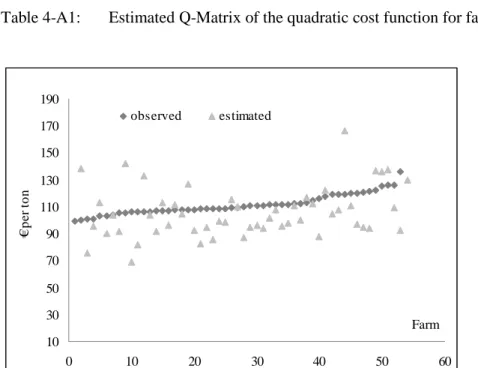
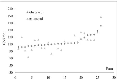
Chapter 4 develops an estimation method for the specification of crop-specific

input coefficients in MP models. The lack of information about input allocations for different crop levels, e.g., fertiliser inputs for wheat or the level of pesticides used for sugar beets, provides a challenge for the specification of aggregated farm type models. In farm accounting records available for farm group models, often only total inputs per farm are reported. In aggregated MP farm type models, the explicit

(10)

representation of input allocation plays an increasingly important role, for example in the representation of environmental effects such as nitrogen intake, and subsequently in the modelling of policy alternatives. In the past, crop-specific inputs were either implemented ad hoc in MP models based on management handbooks, or were based on total input levels that were estimated with input-output regressions. This chapter presents an approach that combines the regression approach with the estimation of a farm supply model using single farm data. The relationship between the MP and the linear regression model is defined, and an estimation approach based on the optimal condition of the farm is presented. The developed estimation approach is applied to Belgian FADN data, where input allocations for various crop levels are collected in the database. A comparison of observed and estimated data is possible to validate the suggested method. The results show that the developed estimation approach successfully models the observed values of input allocation, in contrast to the regression estimation. Furthermore, this approach leads to a crop-specific breakdown of variable inputs and a representation of the resulting farm type with a fully specified non-linear component.

Chapter 5 presents the farm type module developed in the modelling system

CAPRI (Common Agricultural Policy Regional Impact). The integration of farm types into the modelling system CAPRI provides the chance to directly quantify the effects of market policies and developments on the farm level and to reduce the aggregation bias, resulting in an improved localisation of farm type related environmental effects. The farm types in CAPRI are based on data from the European Farm Structure Survey (FSS). For several reasons, these data are not consistent with the CAPRI database. One possible way to overcome these inconsistencies would be a simple linear up- and down-scaling of FSS to the quantity structure of the CAPRI database. However, this method could lead to a loss of information about the type and size of the farm group from FSS. To avoid this effect, an estimation approach is developed covering EU-27 that does not violate the type of farming or the economic size of the farm types.

(11)

The Common Agricultural Policy (CAP) of the European Union led to increased agricultural production in Europe during the 1960s and 1970s, resulting in structural overproduction, expensive storage costs, and negative environmental effects. In the 1980s, the EU began systematic reforms to remove overproduction, consider negative impacts on the environment, and avoid dumping excess production into world markets. At the beginning of the 20th century, the CAP increased its focus on externalities of agricultural production and the contribution of the farming sector to rural development. To satisfy legally required impact assessments (IA) of the European Commission (COM, 2002) and also to support national governments, the research community developed and applied tools to support and accompany the policy-making process. Multi-commodity country-specific models such as those reported in Banse et al. (2004), OECD (2007), and Bartova et al. (2007) were complemented with regionalised assessment tools (see, e.g., Britz & Witzke, 2008; Gömann et al., 2007) as responses to the CAP movement from price to direct income support. However, regionalised supply models consider all farms in a region as a territorial aggregation, which can lead to bias given the evolution and growing importance of policy instruments and legislation and their differential impact depending on individual farm characteristics such as farm revenues, herd sizes, stocking densities, or fertiliser applications. To account for the heterogeneity in the agricultural sector and to be able to conduct IA to evaluate the consequences of policy implementations on the farm level within the various farming systems across Europe, methods in economic farm modelling were developed. Economic farm modelling is based on micro-level data on agricultural firms, and differentiates decision-makers through properties such as crop patterns, type of farming, animal density, economic size, and legal form. The development and evaluation of farm tools for IA requires a great deal of data to represent the heterogeneous structure of the farming level and to infer information on input-output relationships and income. Official statistics for agricultural farm level analysis mainly come in two forms. The first is the Farm Structure Survey (FSS), which aims to survey the structure of agricultural holdings. This survey contains country and regional level information on land use, animal head sizes, and the work force. This survey is available from Eurostat and is collected every three years as a sample survey and every ten years as a complete survey. The second data source is the European Commissions Farm Accountancy Data Network (FADN), which collects accounting information at the farm level and is the most important source when conducting country-wide farm

(16)

related IA. The European FADN is collected annually and is sourced by national accounting data. The two databases are accessible for developing policy IA tools under specific rules that regulate the transmission of data, subject to statistical confidentiality.

1.2 Objectives and methodological approaches

Against this background, the aim of this dissertation is to contribute to the research field of economic farm modelling by developing methods that improve tools for IA of the CAP in Europe. The thesis gives special attention to four different methods in farm economics. The first method deals with the problem of measuring and comparing the performance of farmers, given that a farm produces more than one output and uses more than one input. The heterogeneity of the farming system with respect to the composition and economic size of an individual farm makes it difficult to differentiate economic performance. Data Envelopment Analysis (DEA) as a frontier method defines an efficiency score for a farm relative to the best farms in the sample. The objective of the study is to answer whether DEA as a non-parametric approach yields robust efficiency rankings with respect to statistical significance (Chapter 2). A further topic of this thesis is the assessment of the impact of different calibration methods on the explanatory power of mathematical farm group models, which are often superior to econometric estimated models because they are better able to include policy instruments such as quotas and environmental restrictions (Chapter 3). However, these models need to be calibrated, using Positive Mathematical Programming (PMP) methods. Also, problems of missing information and inconsistent databases arise. One research question results from the lack of information on the input allocation per enterprise. Since input allocation is not available, this study aimed to develop a possible extension of the standard linear regression approach to estimate the input allocation (Chapter 4). Methodological development is also required when confronting the inconsistencies in data sources that are often caused by the statistical confidentiality regulations or by differences in time dimensions and definitions (Chapter 5). The objectives and the methods used to accomplish them are briefly introduced in the remainder of this section.

1.2.1 Efficiency analysis with DEA

In efficiency analysis, each farm receives an efficiency score relative to the best practice, represented by a frontier (Farrell, 1957). There are two main techniques used to estimate the frontier and to calculate the efficiency score - namely, the stochastic frontier approach and DEA. The former uses statistical methods to estimate the frontier and the latter uses mathematical programming to calculate efficiency scores compared to the best observed praxis. The efficiency score is a

(17)

performance indicator. Often, a second stage regression of those scores on explanatory variables such as off-farm earnings and tenure status is used to identify the reasons for the efficiency or inefficiency. The DEA methodology is a technique widely used in agricultural applications. The importance of performing statistical inference on efficiency scores is concerned applying Simar & Wilson’s (2004) smoothed homogeneous bootstrap procedure to investigate bias, variance and confidence intervals for the attained DEA efficiency scores. Based on confidence intervals for efficiency scores, the effect of input aggregation and returns to scale on the efficiency ranking is demonstrated using a statistic that facilitates a comparison of the quality of the efficiency rankings.

1.2.2 Response behaviour of PMP methods

Heckelei & Wolff (2003) have analytically shown the arbitrariness of the response of PMP calibration methods for MP models. Against this backdrop, the effect of the PMP calibration method on the supply response is investigated using the German wide farm model FARMIS1 in an ex post framework. The resulting response of the different calibration methods is compared to the observed behaviour. The approach uses 845 identical farms over eight years from the German FADN; these farms were aggregated into 45 farm groups. The groups are calibrated for the accounting year 1996/97, and the observed gross margins from the year 2002/03 were applied as impacts. All investigated calibration approaches rely on the assumption that an observed production activity of a farm group is the result of profit maximising behaviour. The production economic criterion - marginal revenue equals marginal cost - is used to derive the calibration parameters for the PMP approach. When the PMP methodology was published by Howitt (1995), only the diagonal elements of the additional cost matrix were identified. The first three PMP calibration methods considered in this investigation belong to that group of calibration approaches, and were introduced by Howitt & Mean (1983), Paris (1988), and Helming et al. (2001). The other calibration approaches try to recover cross-activity relationships. The literature has already provided some examples (Paris & Howitt, 1998; Heckelei & Britz, 2000). For this ex post assessment, the maximum entropy techniques proposed by Paris & Howitt (1998) are considered. Furthermore, a method proposed by Heckelei & Wolff (2003) to estimate rather than calibrate the model based on the first order condition, is presented for a selected farm group. Although Jansson (2007) applied a similar method using Bayesian estimation with sector data, this approach represents the first use of time series data from FADN while employing General Maximum Entropy (GME) as an estimator.

1

(18)

1.2.3 Input allocation problem

The ability to explicitly define input demand per activity is one advantage of MP models compared to econometrically estimated farm models with implicit representations of input demand. Additionally, the link between economic models and explicit bio-physical models makes the reliability of input coefficients such as fertiliser and pesticide application rates per crop very important. While official statistics provided in FADN unfortunately do not contain information about the input allocations for production activities, FADN does offer data on the total farm or sector purchases of various input categories. The total amount of inputs per farm and the output per crop were often used to estimate the input allocation for activities by using linear regression (Errington, 1989; Ray, 1985; Midmore, 1990; Léon et al. 1999). Thus, crop-specific inputs in supply models are rarely based on real observations, but instead are estimated before the actual supply model is set up. This regression approach is extended by proposing and applying an innovative estimation approach for farm group programming models using GME. The proposed set-up simultaneously determines the cost function parameters and the input allocations for production activities. This methodology is applied to Belgium FADN data on arable farms, for which the available input allocations allow for a validation of the estimation approach.

1.2.4 Consistent disaggregation of a sector model into farm types

Disaggregation of the supply models of the Common Agricultural Policy Regional Impact model (CAPRI) into farm group models was previously performed by Adenäuer et al. (2006a, 2006b). The major disadvantage of this approach is that during the disaggregation, the farm group data, previously derived from FADN and used as disaggregation information, could lose the characteristics of the type of farming and economic size because regional sectors had to be disaggregated as consistent break-down. This is necessary for maintaining a harmonised database across scales, which allows for an iterative link between supply and market modules. A comparison of the differences between FADN and FSS in comparison to the sector model data has shown that FSS fits the sector model data better. Therefore, an estimation approach is developed to smoothly integrate the information from FSS with the top-down disaggregation approach. FSS is a well-established statistical database that is harmonised across Europe and has suitable coverage by farm type. However, even when using FSS, which itself underlies as source of many of the regional statistics for CAPRI, there are still inconsistencies when compared with regional CAPRI data. First, regional models consider a three-year average, whereas FSS is available for different Member States and different years, so that no three-year average is available. Additionally, regional supply models deviate from official statistics because they are already consistent (e.g., closed market balances), complete

(19)

(i.e., data gaps have been filled using econometric routines), and harmonised over time with regards to product/activity classifications (e.g., aggregation of the cheese or wheat market commodities). Furthermore, regulations on statistical confidentiality define the transmission of FSS data. Specifically, all FSS data on farm groups used as disaggregation information are rounded to the tenth digit, and individual farm data, which accounts for more than 80 percent of a variable, is deleted from the farm group. Production statistics in CAPRI thus differ slightly compared to the original statistics. Therefore, deviations exist between sector models and matching annual FSS data. These inconsistencies in the data could be easily removed by multiplying each production level in FSS with a variable-wise correction factor that is calculated from the given regional level and the sum of the farm types from FSS. However, this approach could first lead to a violation of political requirements for set-aside in the farm groups. Second, and more importantly, correction of activity levels could change the farming patterns such that a different type of farming or a different economic size results. The resulting farm types would no longer represent the actual farming structure observed in FSS. Last but not least, these changes could generate unrealistic farm programs. To avoid this, it is necessary to replace the simple scaling approach with a statistical estimator that ensures regional consistency and compliance with set-aside obligations but prevents changes in the type of farming and economic size of the farm groups. We propose the application of a Bayesian motivated estimation framework that treats the available FSS disaggregated information as a random variable. The disaggregated data provides prior information composed of consistency and definition based conditions. The combination of these parameters provides posterior estimates that fulfil the top-down disaggregation requirement while exhausting the information content of the FSS data. As result the farm type models in CAPRI have two unique attributes. First, the reduction of the aggregation bias leads to more profound impact assessments for farm and agri-environmental related policy changes and reduces the difficulty in bridging results from very highly aggregated models and bio-physical models. Second, the integration of farm types in CAPRI, compared to a standalone farm type approach, gains from endogenous price feedback through the global market model in CAPRI, and enables a direct assessment of the effect of EU-wide market policies on farming systems.

1.3 Structure of the thesis

This thesis contains six chapters. Chapter 1 outlines the background, the objective, and the methodological approaches.

Chapter 2 begins with a review of the concept of efficiency, explains the

(20)

confidence intervals in Section 2.2, and introduces model specification and summary statistics in Section 2.3 that are used to measure the degree of overlapping confidence intervals. Section 2.4 then discusses the estimation results. The final section concludes and points to promising future research opportunities. The author’s interest in the research topic of this chapter began during his study at the Imperial College at Wye, where his master’s degree focused already on DEA methods. The work presented in this chapter and the resulting publication is mainly the outcome of the work the author did during his time at the von Thünen Institute (former FAL) Institute for Farm Economics in Braunschweig. The paper of this chapter has been published as Gocht & Balcombe (2006) in Agricultural Economics.

Chapter 3 investigates the response behaviour of selected PMP approaches using

an ex post framework on German FADN time series data from 1996/97 to 2002/03. After the introduction, Section 3.2 explains the concept of PMP and points out the methodology used to calibrate MP farm models to observed production. The following Section 3.3. describes the ex post approach by first describing the methods used to calibrate the parameters of the cost function, and then introduces the data and discusses implementation of the calibration methods. Afterwards, Section 3.4 discusses the findings and conclusions are drawn in Section 3.5. This chapter is a modified version of Gocht (2005) published as part of the proceedings of the 89th European Seminar of the European Association of Agricultural Economists. Although relevant literature that emerged after this article’s publication was included in the current chapter, the ex post evaluation was not further developed since publication.

Chapter 4 proposes and applies an innovative estimation approach for farm group

programming models using GME. After the introduction Section 4.2 reviews the literature. Section 4.3 presents the derivation of the conceptual farm group model. Section 4.4 develops the empirical model based on the aforementioned discussion, introduces the data, and describes the estimation approach. A discussion about Non-sample information is also included. Section 4.5 evaluates how the simultaneous estimation of input allocations and behavioural models compares with a separate linear regression, as employed in the literature. The results are discussed with respect to the resulting input allocation and the fit of the behavioural model. Furthermore, a sensitivity analysis of the results is performed in order to validate the support point design. Section 4.6 concludes the chapter and discusses further promising research directions. A prior version of this work was presented at the 107th EAAE Seminar by Gocht (2008). The current version of the chapter was developed with T. Heckelei and submitted to the Journal of Agricultural Economics.

Chapter 5 motivates and explains the EU-wide farm type model in CAPRI through its characterisations and develops an estimation approach to consistently disaggregate the sector models in CAPRI into farm type models using FSS. The chapter starts with an introduction and continues with the motivation for the

(21)

development of the model with respect to agricultural policy. Section 5.3 discusses the characteristics of the farm types in CAPRI. The disaggregation problem is outlined in Section 5.3.1, which follows a detailed discussion on the layout of the disaggregation estimator by starting with data constraints before defining the estimator. Section 5.5 presents the FSS data and presents a comparison to FADN data. Section 5.6 analyses the extent to which the proposed estimator leads to an improved presentation of the farming structure by comparing the finding to a fixed variable-wise number scaling approach. Section 5.7 discusses the results and draws conclusions. A report about the farm types in CAPRI will be available in Gocht (forthcoming). Furthermore, Adenäuer et al. (2006a) and Adenäuer at al. (2006b) are prior studies closely related to the work presented in this chapter. The paper of the chapter was written with W. Britz (University of Bonn) and has been submitted for a special issue organised by JRC-IPTS Seville for the Journal of Policy Modelling.

At the end Chapter 6 concludes and identifies areas worth further investigation.

1.4 References

Adenäuer, M., Britz, W., Gocht, A., Gömann, H. & Ratinger, T., 2006a. Development of a regionalised EU-wide operational model to assess the impact of current Common Agricultural Policy on farming sustainability. Final Report J05/30/2004 Bonn, Braunschweig, Seville.

Adenäuer, M., Britz, W., Gocht, A., Gömann, H. & Ratinger, T., 2006b. Modelling impacts of decoupled premiums: building-up a farm type layer within the EU-wide regionalised CAPRI model. In: 93rd seminar of the EAAE "Impacts of Decoupling and Cross Compliance on Agriculture in the Enlarged EU" September 22nd-23rd 2006, Prague, Czech Republic. Prague, pp. 24.

Banse. M., Grethe, H. & Nolte, S., 2004. European Simulation Model (ESIM) in GAMS: Model: Documentation. Available at http://wwwuser.gwdg.de /~mbanse/publikationendokumentation-esim.pdf.

Bartova L., M'barek R. & AGMEMOD Partnership, 2007. Impact Analysis of CAP Reform on the Main Agricultural Commodities. Report II AGMEMOD - Member States Results. JRC Scientific and Technical Report. EUR Number: 22940 EN/2. 10/2007. Available at http://www.jrc.es/publications.

Britz, W. & Witzke, P., 2008. CAPRI model documentation 2008. Available at http://www.capri-model.org/docs/capri_documentation.pdf, pp. 181.

COM, 2002. Communication from the Commission on impact assessment, Brussels, 5.6.2002, 276 final. Available at http://eur-lex.europa.eu/LexUriServ/LexUri Serv.do?uri=COM:2002:0276:fin:en :pdf.

(22)

Errington, A., 1989. Estimating Enterprise Input-Output Coefficients from Regional Farm Data. Journal of Agricultural Economics 40, 52-56.

Farrell, M. J., 1957. The Measurement of productive efficiency. Journal of Royal Statistical Society ACXX (3), 253-290.

Gocht, A., 2005. Assessment of simulation behavior of different mathematical programming approaches. In: Arfini Filippo (ed.). Modelling agricultural policies: state of the art and new challenges; proceedings of the 89th European Seminar of the European Association of Agricultural Economists (EAAE), Parma, Italy, February 3rd-5th, 2005. Parma : Monte Universita Parma Editore, pp. 166-187.

Gocht, A. & Balcombe, K. 2006. Ranking efficiency units in DEA using bootstrapping an Applied analysis for Slovenian farm data. Agricultural Economics 35, 223-229.

Gocht, A., 2008. Estimation input allocation for farm supply models, In: EAAE Seminar: Modeling of Agricultural and Rural Development Policies. Sevilla (Spain), January 29th -February 1st, 2008, pp. 31.

Gocht, A., (forthcoming). Update of a quantitative tool for farm systems level analysis of agricultural policies (EU FARMS) Final Report. JRC-Scientific and Technical Report. Seville, http://www.jrc.es/publications, pp. 101.

Gömann, H., Kreins, P. & Müller C., 2004. Impact of nitrogen reduction measures on nitrogen surplus, income and production of German agriculture. Water Science & Technology 49(3), 81–90.

Heckelei, T., & Britz, W., 2000. Positive Mathematical Programming with Multiple Data Points: A Cross-Sectional Estimation Procedure. Cahiers d'Economie et Sociologie Rurales 57, 28-50.

Heckelei, T. & Wolff, H., 2003. Estimation of Constrained Optimisation Models for Agricultural Supply Analysis Based on Generalised Maximum Entropy. European Review of Agricultural Economics 30(1), 27-50.

Helming, J. F. M., Peeters, L. & Veendendaal, P. J. J., 2001. Assessing the Consequences of Environmental Policy Scenarios in Flemish Agriculture. In: Heckelei, T., H. P. Witzke & W. Henrichsmeyer (eds.). Agricultural Sector Modelling and Policy Information Systems. Proceedings of the 65th EAAE Seminar, March 29 31, 2000 at University of Bonn, Vauk-Verlag Kiel, pp. 237- 45.

Howitt, R. E. & Mean, P., 1983. A Positive Approach to Microeconomic Programming Models, Working Paper (6). Department of Agricultural Economics, University of California, Davies.

(23)

Howitt, R. E., 1995. Positive Mathematical Programming. American Journal of Agricultural Economics 77(2), 329-42.

Hüttel, S., Küpker, B., Gocht, A., Kleinhanß, W., Offermann, F., 2006. Assessing the 2003 CAP reform impacts on German agriculture. Schriften der Gesellschaft für Wirtschafts- und Sozialwissenschaften des Landbaues 41, 293-303.

Isermeyer, F., Gocht, A., Kleinhanß, W., Küpker, B., Offermann, F., Osterburg, B., Riedel, J. & Sommer, U., 2005. Vergleichende Analyse verschiedener Vorschläge zur Reform der Zuckermarktordnung : eine Studie im Auftrag des Bundesministeriums für Verbraucherschutz, Ernährung und Landwirtschaft. Braunschweig : FAL, pp. 116, Landbauforschung Völkenrode: Special Issue 282.

Jansson, T., 2007. Econometric specification of constrained optimization models. Ph.D. Thesis, Universität of Bonn. Available at http://hss.ulb.uni-bonn.de /diss_online/, pp. 162.

Kleinhanß, W., Gocht, A. & Kovacs, G., 2006. Assessing the impacts of the CAP reform in Hungary and Germany. In: Sandor M. & Laszlo D. (eds.). 10. Nemzetközi agrarökonomiaiudomanyos napok "Agraralkal mazkodas a valtozo gazdasaghoz", Gyöngyös, 2006, marcius 30-31. Gyöngyös : no pub., pp. 8. Léon, Y., Peeters, L., Quinqu, M., & Surry, Y., 1999. The use of Maximum Entropy

to estimate Input-Output coefficients from regional farm accounting data. Journal of Agricultural Economics 50, 425-39.

Midmore, P., 1990. Estimating Input-Output Coefficients from Regional Farm Data. Journal of Agricultural Economics 41, 108-11.

OECD, 2007. Documentation of the AGLINKCOSIMO model. Available at http://www.olis.oecd.org/olis/2006doc.nsf/LinkTo/NT00009066/$FILE/JT0322 3642.PDF.

Offermann, F., Gocht, A., Hüttel, S., Kleinhanss, W. & Kuepker, B., 2006. Assessing The Impacts Of The 2003 Cap Reform In Different EU Member States, presented at the annual conference of the 80th Agricultural Economics Society, 30th and 31st March 2006 PARIS, France.

Paris, Q., 1988. PQP, PMP, Parametric Programming and Comparative Statics. Chapter 11 in Notes for AE 253. Department of Agricultural Economics, University of California, Davis.

Paris, Q. & Howitt, R. E., 1998. An Analysis of Ill-Posed Production Problems Using Maximum Entropy. American Journal of Agricultural Economics 80(1), 124-38.

(24)

Ray, S. C., 1985. Methods of estimating the input coefficient for linear programming models. American Journal of Agricultural Economics 67, 660-65

Simar, L. & Wilson, P. W., 2004. Performance of the bootstrap for DEA estimators and interating the principle. In: Cooper, W. W., Seiford, L. M., Zhu, J. (eds.). Handbook on Data Envelopment Analysis. Kluver, Norwell, MA, pp. 265-298.

(25)

Chapter 2. Ranking efficiency units in DEA using bootstrapping an applied analysis for Slovenian farm data∗∗∗∗

Abstract

This article explores how data envelopment analysis (DEA), along with a smoothed bootstrap method, can be used in applied analysis to obtain more reliable efficiency rankings for farms. The main focus is the smoothed homogeneous bootstrap procedure introduced by Simar and Wilson (1998) to implement statistical inference for the original efficiency point estimates. Two main model specifications, constant and variable returns to scale, are investigated along with various choices regarding data aggregation. The coefficient of separation (CoS), a statistic that indicates thedegree of statistical differentiation within the sample, is used to demonstrate the findings. The CoS suggests a substantive dependency of the results on the methodology and assumptions employed. Accordingly, some observations are made on how to conduct DEA in order to get more reliable efficiency rankings, depending on the purpose for which they are to be used. In addition, attention is drawn to the ability of the SLICE MODEL, implemented in GAMS, to enable researchers to overcome the computational burdens of conducting DEA (with bootstrapping). JEL classifications: C15, D31, Q10

Keywords: Data envelopment analysis; Bootstrapping; Agriculture; Technical efficiency; Confidence intervals; Slice DEA model; GAMS

2.1 Introduction

Data Envelopment Analysis (DEA) is a potentially useful technique for measuring efficiency. But some concerns need to be addressed before DEA can be accepted as a routine tool in applied analysis. Since DEA is an estimation procedure which relies on extremal points, it could be extremely sensitive to data selection, aggregation, model specification and data errors. These points must be borne in mind when investigating the efficiency of farms. Since DEA is a technique which is widely used in agricultural applications, this paper aims to show the importance of performing

∗_{This paper has been published together with K. Balcombe in Agricultural Economics 35 (2006)}

(26)

statistical inference on efficiency scores in that context, because the performance of farms can be heavily influenced by measurement errors and effects like weather, shocks and diseases. Furthermore most agricultural scientists have ignored the sampling noise in DEA estimates, despite the growing literature on the statistical properties of DEA estimators.

Therefore, this paper addresses how the Simar and Wilson (SW) smoothed homogeneous bootstrap procedure1 can be used to investigate bias, variance and confidence intervals for the attained efficiency scores in order to get more reliable efficiency rankings. Based on the confidence intervals for the efficiency scores, it is demonstrated how the choice of input aggregation and returns to scale affect the ranking of the Decision Making Units (DMU). A Slovenian data set will serve as the background against which these issues are discussed. To analyse the findings, a statistic called coefficient of separation (CoS) is introduced, which facilitates a comparison of the quality of the efficiency rankings for the sample farms used in the investigation. In addition, attention is drawn to the ability of the SLICE model, implemented in GAMS, to enable researchers to overcome the computational burdens of conducting DEA (with bootstrapping).

The article is structured as follows: in Section 2.2, the “concept of efficiency” is introduced briefly along with some history regarding DEA analysis. Further, the statistical model and the smoothed homogeneous bootstrap procedure are reviewed briefly. In Section 2.3, the data, the model specifications and the methods used to compare the findings are introduced. Finally, the findings are discussed in Section 2.4, along with implications for the practical implementation of DEA. At the end, conclusions are drawn and areas worth further investigation are identified.

2.2 Methods

2.2.1 The concept of efficiency

The concept of economic efficiency is generally assumed to consist of two components: technical efficiency and allocative efficiency. Broadly, the former is defined as the capacity and willingness of an economic unit to produce the maximum possible output from a given bundle of inputs and technology. The latter is defined as the ability and willingness of an economic unit to equate its specific marginal value

1

Bootstrap procedures suggested by Ferrier and Hirschberg (1999) or Löthgren (1998) are not taken into account, because SW (1999a, 1999b, 2000) have shown that these procedures give inconsistent estimators.

(27)

product with its marginal cost. Farrell (1957) developed an isoquant method to measure efficiency in frontier models. He suggested either the use of a nonparametric piecewise linear convex isoquant or the use of a parametric function fitted to the data in a way that no point should lie to the left of or below the frontier.

Farrell (1957) introduced technical efficiency as a relative notion, relative to best-observed practices in the group. To get the “relative” technical efficiency of the kth firm, we have to calculate the actual output divided by the maximum feasible observable output. Because the actual output is observable, the maximum output must be estimated. To get the maximal output, there are different methods.

The majority of early economists followed a parametric approach. However, economists at Berkeley advanced a programming approach for piecewise linear frontier production functions that went largely unnoticed by the research community (Forsund and Sarafoglou, 2002).

Charnes et al. (1978) (CCR) showed that the Farrell unit isoquant model was a special case of the ordinary linear programming problem. At first, in operational research and management science, but later also within economics, CCR started a new active research field, popularly called DEA. For the applied economists, the great advantage compared to the aforementioned frontier approaches was the possibility for using multiple outputs in a primal approach. DEA encompasses a variety of related models for evaluating performance of the DMU. Another advantage of the DEA approach is that it places no restrictions on the functional form of the frontier and it does not impose any (explicit) distributional assumption on the firm specific efficiency. DEA can accommodate multiple outputs and inputs but is extremely sensitive to variable selection and errors.

DEA focuses on deriving results for each DMU. On the other hand, the stochastic frontier analysis (SFA) approach, as originally proposed by Aigner et al. (1977) and subsequent refinements (e.g., the Bayesian Frontier Approaches in Fernández et al., 1997, 2000, and classical approaches in Coelli et al., 1998), of this model can test hypotheses about the underlying technology and determinants of efficiency. Banker (1996) and Grosskopf (1996) collectively provide a survey of statistical inference on nonparametric, deterministic, linear programming-based frontier models. Several researchers have tried to compare results of applications of different estimation methods based on the same set of data. De Borger and Kerstens (1996) and Bauer et al. (1998) attempt to give guidelines about what sort of methodology should be employed. Banker et al. (1985), Sharam et al. (1999), and Plessmann (2000) compared DEA with other estimation methods, whereby the structure of production was unknown. Gong and Sickles (1992) utilized Monte Carlo techniques to control the underlying technology and compared SFA with DEA. The overarching conclusion is that if the functional form is close to the underlying technology, SFA outperforms DEA. However, DEA seems to be more appropriate when the knowledge about the underlying technology is weak (Kalirajan and Shand, 1999). The practical advantage

(28)

of dealing with multiple outputs is also very real. While stochastic frontier multiple-output “distance functions” have been estimated in the literature (Morrison Paul et al., 2000), the choice and use of appropriate instruments to deal with problems of endogeneity has not been sufficiently addressed.

From these surveys, it becomes evident that for DEA to be viewed as a true competitor to SFA, point estimates of efficiencies are not enough. Fortunately, there is now a considerable body of research that has characterised the statistical property of DEA estimators. SW (1998) proposed a general methodology for bootstrapping in frontier models to conduced confidence intervals, and in subsequent articles (e.g., SW, 2000a, 2000b) the method has been further elucidated and developed. More recent work has also examined the properties of two-step estimators explaining efficiency and adaptations of the standard bootstrap (SW, 2003). However, the question of which method, SFA or DEA, is the best very much dependent on the nature of and knowledge about the data-generating process (DGP). Without a priori knowledge of the DGP, a nonparametric approach such as DEA would seem to have distinct advantages, since the constraints that it imposes on the technology are arguably less severe than parametric methods. Nevertheless, the choice of DEA does not completely decide on the nature of model choice. The premise of this article is that there is still room for guidance on the nature of model choice, particularly with regard to the choice of constant return to scale (CRS) or variable returns to scale (VRS), and its subsequent impact on the confidence intervals derived from bootstrapping.

Finally, from a practical point of view, the application of bootstrapping methods needs to be efficient in terms of computational time. Within the economics literature, the applications of bootstrapping methods have been constrained for this reason. With standard approaches, DEA becomes excessively time consuming to bootstrap as the sample size grows (growing at a rate approximately related to the sample size squared). Here, unlike most existing studies, we employ the SLICE module within GAMS. When using this method, computational expense can no longer be considered a reason for not conducting statistical inference on DEA results with bootstrapping.

2.2.2 Bootstrapping in DEA

Bootstrapping is a method of testing the reliability of a data set by creating a pseudo- replicate data set. Bootstrapping allows you to assess whether the distribution has been influenced by stochastic effects and can be used to build confidence intervals for point estimates, which normally cannot be derived analytically. Random samples are obtained by sampling with replacement from the original data set, which provides

(29)

an estimator of the parameter of interest. SW (1998)2 introduced a DEA bootstrap where the DGP is repeatedly simulated by re-sampling the sample data and applying the original estimator to each simulated sample. The bootstrap method is based on the idea that the bootstrap distribution will mimic the original unknown sampling distribution of the estimators of interest (using a nonparametric estimate of their densities). Hence, a bootstrap procedure can simulate the DGP by using Monte Carlo approximation and may provide a reasonable estimator of the true unknown DGP.

The efficiency for a given point (x y_k, _k)is

{

}

min | ( )

k xk X yk

θ = θ θ ∈

where X y( _k)is a input requirement set. If θ_k =1, the unit k is input efficient.

1 k

θ ≤ represents the feasible proportionate reduction of inputs the DMU could realize, if y were produced efficiently. SW (1998) denote the efficient level of input _k

corresponding to the output levely as_k x xθ( _k|y_k)=θ_kx_k. Note thatθ_kis a radial measure of the distance between (x y_k, _k) and the corresponding frontier. Unfortunately,θ_kis unknown because X y and ( ) θ_kx_kare unknown.

2.2.3 The data generating process

Suppose the DGP, P generates a random sampleχ=

{

(

x_k,y_k|k=1,...,n

)

}

. Using the data χ with a nonparametric method

1 1 1 ˆ _min _| n _| n _| n _1, _{0 |} _{0 |} _1,..., k k i i k i i i i i i i y y x x i n θ θ γ θ γ γ γ θ = = =   =  ≤ ≥ = ≥ ≥ =  

∑

. (2.1)

To obtain ˆX y( ), ∂X yˆ( ), it is possible to estimate its efficiency

{

}

ˆ _min _| ˆ₍ ₎

k xk X yk

θ = θ θ ∈ .

Because the DGP P is unknown, the bootstrap procedure is used to determine the DGP ˆP as a reasonable estimator of the true unknown DGP generated through the

dataχ. The efficiency estimates can be considered as a new population, from which it is possible to draw a new data set

(

)

{

}

* *_, * _| _1,..., i i x y i n χ = = .

This pseudo-sample defines the corresponding quantities Xˆ ( )* y and ∂Xˆ ( )* y . Note that conditionally onχ, the sampling distribution of the estimators Xˆ ( )* y and

2

(30)

* ˆ ( )

X y

∂ are known, since ˆP is known. Analytically, ˆP could be difficult to

compute, therefore Monte Carlo Approximation is employed to obtain the sampling distributions using ˆP to generate B pseudo-samples *

b

χ , where b =1, …, B and

estimates of the efficiency scores. The empirical distribution of these pseudo-estimates gives an approximation of the unknown sampling distribution of the efficiency scores.

2.2.4 Smoothed bootstrap procedure

Unfortunately, this "naïve" bootstrap yields inconsistent estimates. Therefore, SW introduced a homogeneous smoothed bootstrap procedure. An easily implemented algorithm for consistently generating the bootstrap values θˆ_b*from a kernel density estimate is given in SW (1998) and is summarized in the following steps:

(a) First, for each DMU k given the input-output data (x y_k, _k) k=1,...,n, compute ˆ

k

θ by the linear program to get the efficiency estimators. Here the linear model specifications are different estimators of the same unknownθ_k. Hence,

ˆ k

θ estimators are random variables and merely specific realizations of different random variables.

(b) Generate the smoothed bootstrap sample θ₁*,...,θ_n*for i=1,...,n by letting

* *

1 ,..., n

β β , a simple bootstrap sample from θˆ₁*,...,θˆ_n*obtained by drawing uniformly with replacement.

Define sequences * * * * * * * if 1, 2 otherwise i i i i i i i h h β ε β ε θ β ε  ₊ ₊ _≤   =  − −     ɶ _, _(2.2)

and obtain the corrected bootstrap sample by

) ~ )( ˆ / 1 /( 1 ˆ2 * * 2 * *

β

σ

θ

β

θ

_i = + +h _θ i − , (2.3)

with β*=1 /n

∑

_in₌₁β_i* and σˆ_θˆ2 is the sample variance of

* *

1 ˆ _,..., ˆ

n θ θ .

Making these corrections ensures that the sample values have the same mean and variance as the original values. Here h is called the bandwidth factor and

* i

ε is a random deviate drawn from the standard normal. SW discussed in detail how to calculate the bandwidth factor. If the data ( ˆθ) is normal

(31)

distributed, then one may use the normal reference rule and set the bandwidth by 1/5 ˆ ˆ _1.06_ˆ h= σ_θn−

In cases where the data is not normal distributed, as in the case of DEA estimates, SW (2004) suggested the to employ least square cross-validation, which involves choosing the bandwidth that minimizes an approximation to mean integrated square error; see Silverman (1986) for details. In order to obtain h in our study, the least square cross-validation approach3 was applied. (c) Next, use the smoothed bootstrap sample sequence to compute new data

(

)

{

}

* * , | 1,..., b xib yi i n χ = = , where

{

}

* _ˆ _ˆ* ( / ) , 1,..., ib i ib i x = θ θ x i= n and

(d) compute the bootstrap efficiency estimates

{

_{ˆ |}*

}

1, ,

i i n

θ = …

by solving the DEA model for each DMU but using the new dataχb*. For example, for DMU k the bootstrap estimates θˆ*_{k b}_, can be obtained by solving

* * , , 1 1 1 ˆ _min _{0 |} n _| n _| n _1, _{0, ,...,} k b k i i k i i b i i i i i y y x x i n θ θ γ θ γ γ γ = = =   =  > ≤ ≥ = ≥  

∑

. (2.4)

Finally, repeat step (b)-(d) B times to provide for k =1,…, n a set of estimates

{

*

_}

,

ˆ _1,...,

k bb B

θ = .

In our case, we set B = 2,000 to ensure adequate coverage of the confidence intervals. The bootstrap efficiency scores θˆ_k* represent approximations to the ˆθ_k, just as the DEA efficiency scores ˆθ_krepresent approximations to θ_k.

3

(32)

2.2.5 Bootstrap bias corrections

The empirical bootstrap distribution can be used to estimate the bias. An estimate of the bias is defined as the difference between the empirical mean of the bootstrap distribution and the original efficiency point estimates. As shown above, the bootstrap estimates {θˆ_{k b}*_, =1,..., }B are biased by construction (SW, 2000a).

By definition,

( ) ( )

ˆ ˆ

k k

BIAS θ =E θ −θ

the empirical bootstrap bias for the original estimator ˆθ_k is therefore

1 * , 1 ˆ ˆ ˆ ( ) B B k k b k b BIAS θ B− θ θ =   =  − 

∑

 .

The bias-corrected estimator is obtained by subtracting the bias from the original efficiency estimates. However, the bias correction introduces additional noise and could have a higher mean square error than the original point estimates, which can be avoided for the interval estimation using the automatic correction below.

2.2.6 Confidence intervals

To find confidence intervals, SW proposed the modified percentile method. They introduce an improved procedure to derive confidence intervals, which automatically corrects for bias without explicit use of a noisy biased estimator. Using the bootstrap score, we can build confidence intervals for each k. If we know the distribution of

( ) ( )

(

_ˆ*

)

, ,

x y x y

θ −θ , it would be possible to find a b_α, _αsuch that

α

θ

α α ≤ − ≤− = − − ˆ ( , ) ( , ) ) 1 Pr( b k x0 y0 x0 y0 a (2.5)

Because a b_α, _αare unknown, we use

{

*

}

,

ˆ _1,...,

k bb B

θ =

to find values ˆb a_α,ˆ_αsuch that *

, 0 0 0 0

ˆ ˆ ˆ _ˆ ˆ

Pr(− ≤b_α θ_{k b}(x y, )−θ_k(x y, )≤ −α_α | (P χ_n)) 1= −a. (2.6) Finding ˆb a_α,ˆ_α entails sorting the values θˆ*_{k b}_, ( ,x y₀ ₀)−θˆ_k(x y₀, ₀), b =1,…, B in increasing order and then deleting [( / 2) 100]%α × of the rows at either end of the list and setting −bˆ_α,−aˆ_αto the endpoints of the array withaˆ_α ≤bˆ_α. The 1−α percent confidence interval is then;

(33)

0 0 0 0 0 0 ˆ

ˆ _{( ,} ₎ _ˆ _{( ,} ₎ ˆ _{( ,} ₎

k x y aα x y k x y bα

θ + ≤θ ≤θ + _. _(2.7)

This procedure is repeated n times to obtain n confidence intervals, one for each

farm. As a side note, the ˆa_α ≤0,b_α ≤0 and the ˆθ_kwill lie above the confidence interval. For proof, see Voelker (2002).

2.3 Data and model specification

2.3.1 Data

This article uses Slovenian farm cross-sectional data to investigate how efficiency ranking depends on the model specifications and how confidence intervals can be used to give further insights into the validity of the efficiency scores. The data used in this study is based on the Research Institute for Agricultural and Food Economics farm cost database in Slovenia in 1996. Sixty-nine Slovenian arable farms were selected for the investigation. After the data set was corrected for outliers, the mean normalized procedure (Sarkis, 2002) was applied. The four inputs are (1) purchased seed, home grown seed; (2) purchased fertilizer, manure; (3) chemicals, other direct costs, wages; and (4) services and other cost (all inputs are in monetary terms). Output was defined as production of wheat in metric tons.

2.3.2 Coefficient of separation

In order to provide a summary statistic of the degree of overlap between confidence intervals, a useful measure is introduced in this study, which is called “the CoS” (Latruffe et al., 2005). This statistic is calculated by taking each farm in turn and then identifying the farms in the sample that are significantly more efficient than it, that is to say the farms with a lower bound strictly greater than the upper bound for the farm in question.

More precisely, let N_n= no. of farms “significantly” greater than n other farms where n=1, 2, ...N−1and N=total number of farms. Thus, N₁=is the number of farms significantly greater than one farm, N₂is the number of farms significantly greater than two farms. Under perfect separation, we would observe

(

)

n

N = N−n , (2.8)

for n=1, 2...N−1. Noting the identity

(

)

1 1 2 1 1 2

∑

− + = − = N n N N N n , (2.9)

(34)

a “CoS” can be constructed as 1 2 1 2 N 1 n n CoS N N N − = =

∑

+ . (2.10)

Under perfect separation this will be one from the identity above

(

)

1 2 1 2 1 1 N n CoS N n N N − = =

∑

− + = . (2.11)

Obviously, if N_n=0for all N , then CoS=1 /N(nearly zero for a large number of farms). Hence, the CoS is a summary statistic which is calculated by taking each firm and identifying the farms in the sample that are significantly more efficient (at a given significance level). The statistic tells us (approximately) what percentage of the sample is significantly less efficient than a given percentage of the sample, after the sample has been ranked. The CoS serves to demonstrate the fact that wider intervals mean higher probability of overlapping intervals. In essence, the smaller the CoS (at a given level of significance), the less we can differentiate between farm efficiencies, given the confidence intervals obtained by the bootstrap.

2.4 Estimation and results

DEA was performed using both CRS and VRS for a 2-input/1-output and 4-input/1-output case. For the 2-input cases, the inputs 1/2 and 3/4 were aggregated. The confidence intervals and the bias-corrected efficiencies were estimated using the homogeneous smoothed bootstrap procedure introduced in previous sections with 2,000 bootstrap draws.

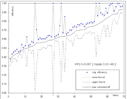
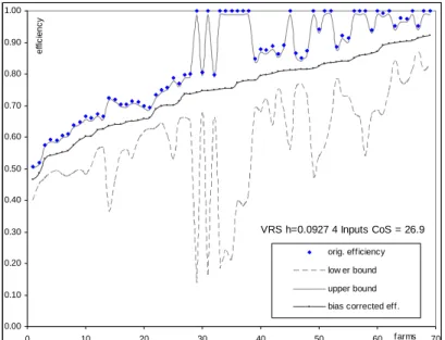
The results for the estimated confidence interval for the 2-input case, VRS/CRS, are shown in Fig. 2-1.

(35)

Fig. 2-1 a: Confidence intervals and point estimates for VRS with two inputs

Fig. 2-1 b: Confidence intervals and point estimates for CRS with two inputs. Fig. 2-1 depicts the sample observations ordered by the bias-corrected efficiency score. The 95% confidence intervals for each farm are represented by the lower dashed line and the upper solid line, and original efficiencies are indicated by the respective symbols. It is evident that the original efficiencies are not included in the confidence interval. This result is not dependent on any particular DGP and is an

Methods in Economic Farm Modelling

Methods in Economic Farm Modelling

Acknowledgements

Kurzfassung

Methoden zur ökonomischen Modellierung landwirtschaftlicher

Betriebe

Abstract

Methods in Economic Farm Modelling

Table of contents

{

}

{

(

)

}

∑

∑

∑

{

}

(

)

{

}

β

σ

θ

β

θ

∑

(

)

{

}

{

}

{

}

∑

∑

∑

{

}

( ) ( )

∑

( ) ( )

(

)

α

θ

θ

{

}

(

)

(

)

∑

∑

(

)

∑

_}