Bayesian Mixture Models For Semi-Supervised Clustering

HAL Id: hal-02372337

https://hal.archives-ouvertes.fr/hal-02372337

Submitted on 20 Nov 2019

HAL

is a multi-disciplinary open access

archive for the deposit and dissemination of

sci-entific research documents, whether they are

pub-lished or not. The documents may come from

teaching and research institutions in France or

abroad, or from public or private research centers.

L’archive ouverte pluridisciplinaire

HAL

, est

destinée au dépôt et à la diffusion de documents

scientifiques de niveau recherche, publiés ou non,

émanant des établissements d’enseignement et de

recherche français ou étrangers, des laboratoires

publics ou privés.

Bayesian Mixture Models For Semi-Supervised

Clustering

Amine Echraibi, Joachim Flocon-Cholet, Stéphane Gosselin, Sandrine Vaton

To cite this version:

Amine Echraibi, Joachim Flocon-Cholet, Stéphane Gosselin, Sandrine Vaton. Bayesian Mixture

Mod-els For Semi-Supervised Clustering. 2019. �hal-02372337�

Bayesian Mixture Models For Semi-Supervised

Clustering

Amine Echraibi

,

Joachim Flocon-Cholet

,

St´ephane Gosselin

, and

Sandrine Vaton

1

_{Orange Labs, France.}

_{

_{amine.echraibi, joachim.floconcholet, stephane.gosselin}

_}

_@orange.com

_{IMT Atlantique, France. [email protected]}

Abstract. In most real-world applications of clustering, data is par-tially labeled by an expert. Classical clustering approaches have been extensively studied in the presence of partial labels, however little work has been done to treat the general case of Bayesian mixture models. In this paper, we propose a new approach to perform semi-supervised clustering using parametric and non parametric mixture models. We show how our approach generalizes mixture models with different types of emission distributions and priors under the same theoretical framework for semi-supervised clustering. The partial la-bels intervene in the clustering in the form of a Hidden Markov Ran-dom Field (HMRF) that introduces a penalty if the partial labels are not respected. We demonstrate how to perform inference in both the finite and infinite case with priors on the mixture components and the parameters using variational inference. Our experimental evalu-ations on synthetic data show how the method can leverage the par-tial labels to choose the correct clustering and the correct number of clusters. We also show that by introducing a small fraction of partial labels our method improves the clustering accuracy and outperforms a strong baseline in the literature on benchmark datasets.

1

Introduction

Semi-supervised learning gained considerable interest from re-searchers recently due to the availability of large amounts of unla-beled data and a small fraction of launla-beled data [7]. A sub task of semi-supervised learning is semi-supervised clustering i.e clustering on partially labeled datasets. These partial labels are usually set by an expert who spent considerable time working on the data and develop-ing some knowledge about the domain [1]. Although this knowledge represented by the partial labels is limited, it could be useful during the clustering analysis. These partial labels can help to identify the number of clusters or the correct view of the clustering, for example. In the semi-supervised learning literature, two approaches to as-sign classes to samples with prior knowledge have been extensively studied. The first approach supposes that all the different classes are present in the labeled part of the dataset, thus the number of classes is known. The model then attempts to propagate the labels to the un-labeled set, by respecting some notion of similarity. Two noteworthy methods of such kind are Transductive Support Vector Machines [10] and label propagation [4] and [17]. The Transductive Support Vector Machine model leverages the unlabeled data in the learning of the decision boundary between classes unlike classical support vector machines where only the labeled data is used. Label propagation, on the other hand, is a graph based approach where the labeled and

un-labeled data points represent nodes of the graph, and edges represent similarities between the nodes. The known labels are then propagated through the graph to label the unlabeled nodes. However, in some real world applications of data mining and information retrieval, the num-ber of possible clusters is unknown and not all clusters are partially labeled. Therefore, we can not use these methods.

The second approach is based on the classical KMeans clustering algorithm, where constraints are added in order to guide the clus-tering, and improve the performance [13]. The constraints are con-structed from the partial labels, must-link constraints assure that two samples must have the same label, and cannot-link constraints assure that two samples shouldn’t be labeled the same. [2] proposed a Hid-den Markov Random Field (HMRF) formulation of this model and later introduced distance learning to identify relevant features to the clustering [3]. In this approach it is possible to find a hidden cluster not present in the partial labels. However, because it is based on the KMeans algorithm, the number of clusters must be known or some sort of model selection needs to be applied to estimate it. For a detail review of these approaches, we refer the reader to [7].

In this paper, we generalize the semi-supervised clustering ap-proach with Hidden Markov Random Fields to the broader range of Bayesian mixture models. This is particularly interesting from a practical perspective, since in some cases we may need to consider various types of probability distributions for clustering, such as cat-egorical distributions or Dirichlet priors for text clustering. Further-more, by considering Bayesian priors on the mixture weights such as Dirichlet distributions [11] or Dirichlet process priors [6], we can estimate the number of clusters from the data itself.

Our contributions1in this paper are the following:

• We propose a general framework to perform semi-supervised clus-tering with Bayesian mixture models, by introducing a Hidden Markov Random Field prior on the hidden class variables.

• We formulate the pairwise potentials of the HMRF using distances between distributions, which allows for the same definition to be applied to different kinds of mixture models.

• We show how to perform inference on the model using variational inference and the mean field approximation [14].

• We show, in the experiments and results, that our model outper-forms a strong baseline on benchmark datasets. We also show that it is capable of identifying the correct view of the clustering and the correct number of clusters, and how it can also improve per-formance of classical unsupervised Bayesian mixture models.

The remainder of this paper is organized as follows. First, we present the theoretical framework of semi-supervised clustering in the general case of exponential family mixture models. We develop the Hidden Markov Random Field formulation that allows for a gen-eralization over different types of probability distributions. Then, we show how to use variational approximation methods to perform in-ference on the model. Finally, we present some didactic examples to give an intuition on how the model behaves in simple situations, and we show how the semi-supervision can improve the clustering performance of classical Bayesian mixture models.

2

Semi-Supervised Bayesian Mixture Models

2.1

Notations

First we introduce some notations that we will use throughout the paper. Let us consider a datasetx1:N = {xn}Nn=1composed ofN

i.i.d. samples of the random variableX. Letz1:NbeNlatent random variables whereznrepresents the class of samplexn. We denote by

θ1:K the random variables representing the parameters of the emis-sion distributions of the mixture model, and byπthe random vari-ables representing the mixture weights, whereK ∈ N∪ {∞}. We

denote byp_θk the prior on the kthparameterθk. A Bayesian mixture model is defined for allkandnas:

π ∼ Dir(K, α)or GEM(η)

θk ∼ p_θk(·) prior onθk zn|π ∼ Cat(·|π)

xn|zn=k, θ ∼ p_X(·|zn=k, θ) emission distribution where the mixture weightsπfollow a Dirichlet distribution in the case of a finite mixture model, or a Dirichlet process in the case of an infinite mixture. In this case, we adopt thestick-breaking construc-tiondefinition [12] whereπ∼GEM(η)is equivalent to:

∀k βk ∼ Beta(1, η) πk = βk k−1 Y l=1 (1−βl)

In the semi-supervised case, some instances of the dataset are la-beled. Let us denote byl1:Nthe partial labels, whereln∈ {1, ..., K} ifxnis labeled,ln=−1otherwise. For the rest of the paper, to sim-plify notation, we simply write for the probability distribution of a random variableX:pX(x) =p(x).

2.2

Supervision in the form of a HMRF

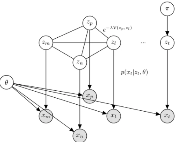
In order to incorporate the information provided by the partial labels into the model, we define a pairwise Hidden Markov Random Field over{z1:N,x1:N}(Figure 1). The HMRF introduces a statistical de-pendency between the random variablesznwith the same labelln:

znneighbor ofzm ⇐⇒ ln=lm

and eachxnis independent ofxmgivenznandθ. We writen∼m

ifznis a neighbor ofzm, The neighborhood of thenth

sample is defined as :

Nn={m∈ {1, ..., N}\{n}s.tm∼n}

The statistical dependency introduced by the neighborhood is later used to construct a joint prior overz1:N in such a way that samples

xn xm xl xp zn zm zl zp xt zt π θ p(xt|zt, θ) e−λV(zp,zl) ...

Figure 1: Overview of the probabilistic graphical model. The unlabeled sam-ples are treated as a classical mixture model wherextdepends onθandzt, andztdepends onπ. The partially labeled samples create dependencies be-tween the hidden variablesz1:N. For each connected pair(zp, zl)we

asso-ciate a factore−λV(zp,zl)_.

in the same neighborhood should be assigned the same label. The definition of the neighborhood can be adapted to other formulations of semi-supervised clustering, such as, the must-link constraint and cannot-link constraints used in [3].

2.3

Semi-Supervised Mixture Models

The Hidden Markov Random Field introduces dependencies be-tween the latent variablesz1:N. The generative process of the semi-supervised mixture model in this case becomes:

π ∼ Dir(K, α)or GEM(η)

θk ∼ p_θk(·) z1:N|π ∼ pz1:N(·|π)

xn|zn=k, θ ∼ pX(·|zn=k, θ)

wherep(z1:N|π)is the joint distribution over the latent variables de-fined by the HMRF. According to the Hammersley–Clifford theorem [8], this joint distribution can be written as :

p(z1:N|π) = 1 Γ N Y n=1 π1[Nn=∅] zn Y n∼m e−λV(zn,zm)

whereV represents the pairwise potentials of the HMRF, andλis a scaling parameter that can be tuned empirically. Given how the HMRF is factored, we can write the normalization constantΓas (proof in appendix B): Γ = X zn,∀ns.tNn6=∅ Y n∼m e−λV(zn,zm)

The main idea behind the HMRF prior, is that neighboring samples should have the same label, otherwise the log-likelihood of the data is penalized by a factor proportional to the pairwise potentials. Other works in the literature proposed various definitions of the potentials, these definitions are often domain or data specific [16]. Others at-tempted to learn these potentials by introducing a parameterized dis-tance [3]. In the following section, we show how to perform inference on the model, and we propose a definition for the potentialsV con-structed from the variational approximating distributions. Therefore this definition can be applied to all types of mixture models.

2.4

Variational Approximation

In order to perform inference on the model, we need to compute or estimate: p(z1:N, θ, π|x1:N)∝p(z1:N,x1:N, θ, π) ∝ N Y n=1 p(xn|zn, θ)p(z1:N|π)p(θ)p(π)

Performing exact inference on this model is intractable. In order to approximate the joint distributionp(z1:N,x1:N, θ, π), we use varia-tional inference and the mean field approximation:

q(z1:N, θ, π) = N Y n=1 q(zn) T Y k=1 q(θk)q(π)

whereT is a truncation level for the number of clusters [6]. The optimal approximate distributionq∗satisfies:

q∗= arg min

q D

KL[q||p] (1)

Solving equation (2) leads to the following mean field update equa-tions:

logq(zn) = const+E{z−n,θ,π}∼q[logp(z1:N,x1:N, θ, π)]

logq(θk) = const+E{z1:N,θ−k,π}∼q[logp(z1:N,x1:N, θ, π)]

logq(π) = const+E{z1:N,θ}∼q[logp(z1:N,x1:N, θ, π)]

By substituting the expression ofp(z1:N,x1:N, θ, π)in the previous equations we have:

q(zn) =Cat(zn;φn) where:

logφnk=const+Eθ∼q[logp(xn|zn=k, θ)] (2) +1[Nn=∅]Eπ∼q[logπk]−λ X m∈Nn T X l=1 φmlV(k, l)

and for the mixture parameters:

logq(θk) =const+ N X n=1 φnklogp(xn|zn=k, θ) + logp(θk) logq(π) =const+ N X n=1 T X k=1 1[Nn=∅]φnklogπk + logp(π)

Usually the prior and the emission distribution are conjugate soq(θk) is in the same exponential family asp(θk). Therefore we can derive fixed point update equations for the variational parameters ofq(π) andq(θk)in the finite and infinite case. However in order to have a closed form for the update equation of the local variational parameter

φnk, we need to propose a definition ofV(k, l), which can be com-puted in close form, and have the property of introducing a penalty in the form of a distance between the clusters. Hence:

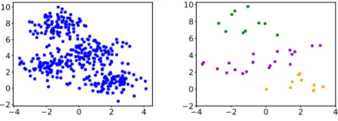
V(k, l),DsymKL [q(θk)||q(θl)] (3) 4 2 0 2 4 2 0 2 4 6 8 10 4 2 0 2 4 2 0 2 4 6 8 10

Figure 2: Samples from 4 Gaussians (left). Partial labels (right).

2.5

Intuition behind the model

The mean field update equations show that the model behaves the same as a classical unsupervised Bayesian mixture model, except in the case of the mean field update forφnk . The first two terms of equation (3) are the same as a classical unsupervised model, where

q(zn = k) depends on the emission probability and the mixture weights. The third term however, introduces the supervision cap-tured in the Hidden Markov Random Field, where for each sample

min the neighborhood ofna penalty is introduced proportional to

φmlV(k, l). Therefore if a samplemin the neighborhood takes a dif-ferent label:l6=k(φml≈1) a penaltyV(k, l)equivalent to the dis-tance between the approximating distributionsq(θk)andq(θl)forces the samples in the same neighborhood to have the same labels. Which in turn constrains the mixture parameters in the following fixed point updates to respect the partial labels.

3

Experiments and Results

We verify through experiments on synthetic data that the model is capable of identifying the correct number of clusters and the cor-rect view of the clustering by leveraging information from the partial labels. We generate 400 samples from a mixture of Gaussian distri-butions of two dimensions. We label a random subset of the samples and we set them as the partial labels. In all the following experiments we adopt the Semi-Supervised Dirichlet Process Gaussian Mixture Model presented in appendix A. In our implementation we initialize the values of the local variational parametersφnkusing the distance from the centers of a fitted KMeans on the data:

φnk∝exp

−1

2||xn−µk||

3.1

Identifying the Correct Clustering

In the first experiment, we generate data from 4 Gaussian distribu-tions, 5 % of the samples of the two clusters at the bottom and the top are labeled, for the two clusters in the middle we label 10 % of all the samples with the same label different from the previous two (Figure 2).

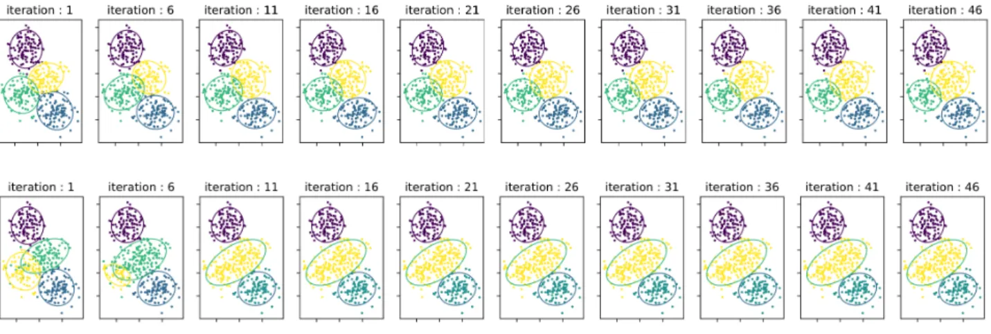
We apply a classical Dirichlet Process Gaussian Mixture Model, and our Semi-Supervised Dirichlet Process Gaussian Mixture Model on this dataset. We set the truncation level of the number of clus-ters toT = 4and then toT = 10, with the same value for the concentration parameterη = 1of the Dirichlet Process. We depict the clustering process across iterations for both the Dirichlet Process Gaussian Mixture Model and our Semi-Supervised Dirichlet Process Gaussian Mixture Model with the truncation level ofT = 4in Figure 3 and forT= 10in Figure 4.

In both cases the semi-supervised DPGMM identifies the correct number of clusters (K= 3) given the partial labels, unlike the classi-cal DPGMM where the number of clusters identified depends on the concentration parameter and the initialization. The intuition gained from this experiment is that the partial labels help the Dirichlet pro-cess to squeeze out unnepro-cessary clusters to explain the data, even if the concentration parameter is high (tendency to produce high num-ber of clusters).

3.2

Identifying the Correct View

In the second experiment, in the same fashion, we generate 400 sam-ples from 4 Gaussian distributions as shown in Figure 6. In this case the clusters are arranged in such a way that ifK = 2, two possible views of the clustering are possible. To identify the correct clustering some information about the view is needed. We suppose that we have two sets of partial labels, and as Figure 7 shows these partial labels encode which view is the correct one in both cases.

We apply the semi-supervised DPGMM in both cases (Figure 5), we set the truncation level of the number of clusterT = 3. We notice that in both cases starting from a KMeans initialization the semi-supervised DPGMM adapts to reach the clustering that respects the view imposed by the partial labels.

3.3

Improving the Clustering Accuracy

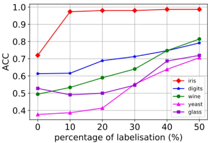
In the last experiment, we apply the semi-supervised DPGMM on the classical UCI datasets (wine, digits, iris, glass, yeast). We consider that the true number of clusters is unknown. We set the truncation level toT = 10for wine, and iris, andT = 20for digits, glass, and yeast. The evaluation metric used to evaluate the clustering is the clustering accuracy [15] defined as :

ACC= max

m∈M

PN

n=11[ln=m(cn)]

N

wherecnis the cluster assignment,lnthe true label andMthe set of all possible one-to-one mappings. we vary the percentage of par-tially labeled samples from 0% (no labels known, fully unsupervised) to 50%, by a step of 10% . On each dataset we report the best accu-racy over 10 reruns of the model, and we plot the evolution of the accuracy for each dataset as a function of the percentage of partial labels (Figure 8). We notice that the clustering accuracy improves as we add labels. For the iris dataset, for example, we notice that the introduction of 20% of the labels improves the accuracy from 72% to 98%. In table 1 we report the clustering accuracy for the classical DPGMM, the semi-supervised DPGMM at 20% of partial labels and at 50% of partial labels. Datasets DPGMM (0%) SS-DPGMM (20%) SS-DPGMM (50%) Iris .72 .98 .98 Wine .49 .58 .81 Glass .52 .5 .71 Yeast .37 .41 .70 Digits .61 .68 .79

Table 1: Accuracy score of the Semi-Supervised Dirichlet Process Gaussian Mixture Model (SS-DPGMM) for multiple percentages of partial labels.

0

10

20

30

40

50

percentage of labelisation (%)

0.4

0.5

0.6

0.7

0.8

0.9

1.0

ACC

Figure 8: Accuracy of the semi-supervised DPGMM on the UCI datasets. The percentage of partial labels varies from 0 to 50 % of the true labels.

3.4

Comparison with HMRF-KMeans

In this section, we compare our approach to the HMRF-KMeans semi-supervised clustering algorithm [3] which is a strong baseline for the semi-supervised clustering task. Similarly to the previous experiment we evaluate the HMRF-KMeans on the classical UCI datasets. We fix the number of clusters to the true number of classes in the dataset and we report the clustering accuracy for different per-centages of partial labels. Figure 9 shows the evolution of the clus-tering accuracy for each dataset.

Our approach clearly outperforms the HMRF-KMeans in terms of clustering accuracy. For example, we can see that for50% labeli-sation the clustering accuracy for all datasets is between [0.5, 0.7], while for our method the accuracy is above 0.7. Furthermore, HMRF-KMeans uses Iterated Conditional modes [5] during the E-Step. This algorithm increases the complexity and therefore the time of exe-cution for each iteration of the EM, unlike our approach, which is based on the classical Variational EM. Our method can identify new separate unlabeled clusters, and thus learn the number of clusters au-tomatically thanks to the Dirichlet Process prior. Unlike the HMRF-Kmeans where the true number of clusters has to be set in advance.

10 15 20 25 30 35 40 45 50

percentage of labelisation (%)

0.2

0.3

0.4

0.5

0.6

ACC

Figure 9: Accuracy of the HMRF-KMeans algorithm on the UCI datasets. The percentage of partial labels varies from 10 to 50 % of the true labels.

Figure 3: Visualization of the clustering process across iterations of the classical DPGMMT = 4(top), and the semi-supervised DPGMMT = 4(bottom).

Figure 4: Visualization of the clustering process across iterations of the classical DPGMMT= 10(top), and the semi-supervised DPGMMT = 10(bottom).

2 0 2 4 6 8 2 0 2 4 6 8

Figure 6: Samples from 4 Gaussian distributions, ifK = 2two views of clustering using a linear boundary are possible: horizontal (two top clusters separated from the bottom clusters) and vertical (the two clusters on the left separated from the clusters on the right).

2 0 2 4 6 8 2 0 2 4 6 8 2 0 2 4 6 8 2 0 2 4 6 8

Figure 7: Partial labels corresponding to the horizontal clustering (left), par-tial labels corresponding to the vertical clustering (right).

4

Conclusion

In this paper, we introduced a new method to perform semi-supervised clustering with Bayesian finite and infinite mixture mod-els. This approach allows the introduction of prior knowledge in the form of partial labels set by an expert to guide the clustering pro-cess towards the correct solution. We have shown that the model can identify the correct view of the clustering and the correct number of clusters, we also demonstrated that by introducing a small fraction of partial labels we can improve the overall accuracy of a classical mixture model. Our approach is general, and can easily be applied to other types of mixture models like the categorical mixture model, latent Dirichlet allocation or topic models. In future work, we will ex-plore how we can extend this approach to more complex probabilistic graphical models. We will also investigate stochastic variational in-ference [9] in order to apply the approach to large scale datasets.

A

Semi-Supervised Dirichlet Process Gaussian

Mixture Model

In this section, we develop the mean field update equations in the case of the Dirichlet Process Gaussian Mixture Model. In what follows we adopt the formulation presented in [11].

The generative process of the model is the following:

∀k βk ∼ Beta(1, η) πk = βk k−1 Y l=1 (1−βl) µk|Λk ∼ N(·|m0,(κ0Λk) −1 ) Λk ∼ W(·;L0, ν0) z1:N|π ∼ pz1:N(·|π) xn|zn=k, µ,Λ ∼ N(·|µk,Λ −1 k )

WhereWis the Wishart distribution. By substituting in the mean field update equations, we have∀k∈ {1, .., T}:

q(βk) = Beta(βk;γ1,k, γ2,k)

q(µk|Λk) = N(µk;mk,(κkΛk)−1)

q(Λk) = W(Λk;Lk, νk)

q(zn) = Cat(zn;φn)

The variational parameters have the following fixed point equations:

γ1,k = 1 + N X n=1 φnk γ2,k=η+ N X n=1 T X l=k+1 φnl κk = κ0+ N X n=1 φnk νk=ν0+ N X n=1 φnk+ 1 mk = κ0m0+PN_n=1φnkxn κk L−_k1 = L−01+κ0(mk−m0)(mk−m0)T + N X n=1 φnk(xn−mk)(xn−mk)T logφnk = − 1 2 d κk +νk(xn−mk)TLk(xn−mk) + 1 2 " _d X i=1 ψ νk+ 1−i 2 + log|Lk| # + ψ(γ1,k)−ψ(γ1,k+γ2,k) + k−1 X l=1 [ψ(γ2,l)−ψ(γ1,l+γ2,l)] − λ X m∈Nn T X l=1 φmlV(k, l) +const

whereψis the digamma function and as defined in (4) the expression ofVis :

V(k, l) =DsymKL [q(µk,Λk)||q(µl,Λl)]

which we can compute in close form as a function of the variational parameters ofq(µk,Λk)andq(µl,Λl), using the standard formulas for the kullback-leibler divergences between two Gaussian distribu-tions and between two Wishart distribudistribu-tions:

V(k, l) = d(κl κk +κk κl −2) +1 2(νk−νl)(log(|Lk|)−log(|Lk|)) + Tr(νkLk+νlLl)(mk−ml)(mk−ml)T + 1 2(νk−νl) " d X i=1 ψ νk+ 1−i 2 # + 1 2(νl−νk) " _d X i=1 ψ νl+ 1−i 2 # + 1 2Tr νkL −1 l Lk+νlL−k1Ll −d 2(νk+νl)

B

The Normalizing Constant

Γ

By definition the normalizing constantΓcan be written as :

Γ = X z1:N N Y n=1 π1[Nn=∅] zn Y n∼m e−λV(zn,zm) = X zn∀n s.tNn6=∅     X zn∀n s.tNn=∅ N Y n=1 π1[Nn=∅] zn     Y n∼m e−λV(zn,zm)

Let’s denote bySthe set containing all points with empty neighbor-hoods : S ={ns.tNn=∅} We have: X zn∀n s.tNn=∅ N Y n=1 π1[Nn=∅] zn = X zn ∀n∈S Y n∈S πzn =Y n∈S X zn πzn = 1 Thus: Γ = X zn,∀ns.tNn6=∅ Y n∼m e−λV(zn,zm)

REFERENCES

[1] Eric Bair, ‘Semi-supervised clustering methods’, Wiley Interdisci-plinary Reviews: Computational Statistics,5(5), 349–361, (2013). [2] Sugato Basu, Arindam Banerjee, and Raymond J Mooney, ‘Active

semi-supervision for pairwise constrained clustering’, inProceedings of the 2004 SIAM international conference on data mining, pp. 333– 344. SIAM, (2004).

[3] Sugato Basu, Mikhail Bilenko, and Raymond J Mooney, ‘A probabilis-tic framework for semi-supervised clustering’, inProceedings of the tenth ACM SIGKDD international conference on Knowledge discovery and data mining, pp. 59–68. ACM, (2004).

[4] Yoshua Bengio, Olivier Delalleau, and Nicolas Le Roux, ‘11 label prop-agation and quadratic criterion’, (2006).

[5] Julian Besag, ‘On the statistical analysis of dirty pictures’,Journal of the Royal Statistical Society: Series B (Methodological),48(3), 259– 279, (1986).

[6] David M Blei, Michael I Jordan, et al., ‘Variational inference for dirich-let process mixtures’,Bayesian analysis,1(1), 121–143, (2006).

[7] Olivier Chapelle, Bernhard Scholkopf, and Alexander Zien, ‘Semi-supervised learning (chapelle, o. et al., eds.; 2006)[book reviews]’,

IEEE Transactions on Neural Networks,20(3), 542–542, (2009). [8] John M Hammersley and Peter Clifford, ‘Markov fields on finite graphs

and lattices’,Unpublished manuscript,46, (1971).

[9] Matthew D Hoffman, David M Blei, Chong Wang, and John Paisley, ‘Stochastic variational inference’,The Journal of Machine Learning Research,14(1), 1303–1347, (2013).

[10] Thorsten Joachims, ‘Transductive inference for text classification using support vector machines’, inIcml, volume 99, pp. 200–209, (1999). [11] Kevin P Murphy,Machine learning: a probabilistic perspective, MIT

press, 2012.

[12] Jayaram Sethuraman, ‘A constructive definition of dirichlet priors’, Sta-tistica sinica, 639–650, (1994).

[13] Kiri Wagstaff, Claire Cardie, Seth Rogers, Stefan Schr¨odl, et al., ‘Con-strained k-means clustering with background knowledge’, inIcml, vol-ume 1, pp. 577–584, (2001).

[14] Martin J Wainwright, Michael I Jordan, et al., ‘Graphical models, expo-nential families, and variational inference’,Foundations and TrendsR

in Machine Learning,1(1–2), 1–305, (2008).

[15] Junyuan Xie, Ross Girshick, and Ali Farhadi, ‘Unsupervised deep em-bedding for clustering analysis’, inInternational conference on ma-chine learning, pp. 478–487, (2016).

[16] Yongyue Zhang, Michael Brady, and Stephen Smith, ‘Segmentation of brain mr images through a hidden markov random field model and the expectation-maximization algorithm’,IEEE transactions on med-ical imaging,20(1), 45–57, (2001).

[17] Xiaojin Zhu and Zoubin Ghahramani, ‘Learning from labeled and un-labeled data with label propagation’, (2002).