Robustness and multivariate
analysis
Fatimah Salem Alashwali
Submitted in accordance with the requirements for the degree of Doctor of Philosophy
The University of Leeds
Department of Statistics
The candidate confirms that the work submitted is her own and
that appropriate credit has been given where reference has been
made to the work of others.
This copy has been supplied on the understanding that it is
copyright material and that no quotation from the thesis may be
published without proper acknowledgement.
Copyright c
2013 The University of Leeds and Fatimah Salem
Alashwali
The right of Fatimah Salem Alashwali to be identified as Author
of this work has been asserted by her in accordance with the
Copyright, Designs and Patents Act 1988.
i
Abstract
Invariant coordinate selection (ICS) is a method for finding structures in mul-tivariate data using the eigenvalue-eigenvector decomposition of two different scatter matrices. The performance of the ICS depends on the structure of the data and the choice of the scatter matrices.
The main goal of this thesis is to understand how ICS works in some situa-tions, and does not in other. In particular, we look at ICS under three different structures: two-group mixtures, long-tailed distributions, and parallel line struc-ture.
Under two-group mixtures, we explore ICS based on the fourth-order moment matrix, ˆK, and the covariance matrix S. We find the explicit form of ˆK, and the ICS criterion under this model. We also explore the projection pursuit (PP) method, a variant of ICS, based on the univariate kurtosis. A comparison is made between PP, based on kurtosis, and ICS, based on ˆK and S, through a simulation study. The results show that PP is more accurate than ICS. The asymptotic distributions of the ICS and PP estimates of the groups separation direction are derived.
We explore ICS and PP based on two robust measures of spread, under two-group mixtures. The use of common location measures, and pairwise differencing of the data in robust ICS and PP are investigated using simulations. The sim-ulation results suggest that using a common location measure can be sometimes useful.
The second structure considered in this thesis, the long-tailed distribution, is modelled by two dimensional errors-in-variables model, where the signal can have a non-normal distribution. ICS based on ˆK and S is explored. We gain insight into how ICS finds the signal direction in the errors in variables problem. We also compare the accuracy of the ICS estimate of the signal direction and Geary’s fourth-order cumulant-based estimates through simulations. The results suggest
ii
that some of the cumulant-based estimates are more accurate than ICS, but ICS has the advantage of affine equivariance.
The third structure considered is the parallel lines structure. We explore ICS based on the W-estimate based on the pairwise differencing of the data, ˆV, and
S. We give a detailed analysis of the effect of the separation between points, overall and conditional on the horizontal separation, on the power of ICS based on ˆV and S.
iii
Acknowledgments
All thanks and praise to Allah for helping me through this journey.
I would like to express my thanks and gratitude to my supervisor Professor John T. Kent for his help, support, and patience during my PhD years. It has been a great pleasure to work with him.
I am profoundly grateful to my husband Abdulaziz for his continuous encour-agement and support. My thanks are also to my children Omar and Albaraa who bring joy to my life.
Lastly, I would like to express my heartfelt thanks and appreciations to my parents, sisters, brothers, nieces and nephews for their support and prayers.
Contents
Abstract i
Acknowledgements iii
Contents iv
List of Figures viii
List of Tables x
1 Introduction 1
1.1 Multivariate analysis . . . 1
1.1.1 Transformations . . . 2
1.1.2 Summary statistics . . . 4
1.1.3 Exploratory data analysis . . . 5
1.2 Location vectors and Scatter matrices . . . 7
1.3 Robust statistics . . . 8
1.3.1 Measuring robustness . . . 8
1.3.2 Robust location and scale estimates . . . 11
1.4 Thesis outline . . . 13
2 Invariant coordinate selection and related methods 16 2.1 Introduction . . . 16
Contents v
2.3 Projection pursuit as a variant of invariant coordinate selections . 19
2.4 Univariate kurtosis . . . 19
2.5 Common location measure . . . 23
2.6 Role of differencing . . . 24
2.7 Types of non-normal structures . . . 24
2.8 How to choose the pair of scatter matrices . . . 25
2.9 Notation . . . 27
3 Using ICS and PP based on fourth-order moments in two-group mixtures 30 3.1 Introduction . . . 30
3.2 The model: Mixtures of two bivariate normal distributions . . . . 31
3.2.1 The model assumptions . . . 31
3.2.2 Univariate moments . . . 34
3.3 Invariant coordinate selection based on fourth-order moments ma-trix in population . . . 38
3.4 Relationship between ICS:kurtosis:variance and Mardia’s multi-variate kurtosis measure . . . 42
3.5 Projection pursuit based on kurtosis in population . . . 43
3.6 A comparison between ICS and PP . . . 45
3.6.1 In population . . . 45
3.6.2 In sample . . . 47
3.7 Axis measure of dispersion . . . 51
3.8 Simulation study . . . 53
3.9 Discussion . . . 56
4 An analytical comparison between ICS and PP 59 4.1 Introduction . . . 59
4.2 The model . . . 60
Contents vi
4.2.2 Moments . . . 60
4.3 The asymptotic theory of sample moments . . . 62
4.4 The asymptotic distribution of the ICS estimates . . . 63
4.5 The asymptotic distribution of PP:kurtosis:variance estimate . . . 69
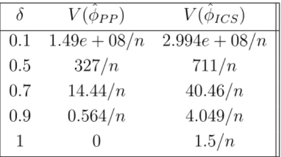
4.6 A comparison betweenV( ˆφICS) and V( ˆφPP) . . . 73
5 Robust ICS and PP 75 5.1 Introduction . . . 75
5.2 The behavior of robust ICS and PP in sample case . . . 76
5.3 Analysis of the problems arising in robust ICS and PP . . . 80
5.3.1 PP:variance:lshorth . . . 80
5.3.2 PP:t2M-estimate:lshorth . . . 82
5.3.3 ICS:t2M-estimate:MVE . . . 84
5.4 Using common location measures . . . 84
5.4.1 PP(Mean):variance:lshorth . . . 84
5.4.2 PP(lshorth):t2M-estimate:lshorth and ICS(MVE):t2M-estimate:MVE 85 5.5 Using pairwise differencing . . . 85
5.5.1 PPd:variance:lshorth and ICSd:variance:MVE . . . . 85
5.5.2 PPd:t 2M-estimate:lshorth and ICSd:t2M-estimate:MVE . . 86
5.6 Conclusion . . . 86
6 ICS in the errors in variables model 89 6.1 Introduction . . . 89
6.2 The errors in variables model . . . 90
6.3 Normal signals . . . 93
6.3.1 Unknown error variances . . . 93
6.3.2 Known error variances . . . 95
6.4 Non-normal signals . . . 97
Contents vii
6.4.2 Joint moments and cumulants . . . 99
6.4.3 Cumulants in EIV . . . 101
6.4.4 The effect of rotation on cumulant based formulas . . . 104
6.5 ICS:kurtosis:variance in EIV . . . 107
6.6 Simulation study . . . 109
6.7 Conclusion . . . 112
7 ICS for RANDU data set 113 7.1 Introduction . . . 113
7.2 ICS for RANDU data set . . . 114
7.2.1 RAND data set . . . 114
7.2.2 RANDU example . . . 115
7.3 Randu-type model . . . 119
7.4 The behaviour ofV in pdimensions . . . 122
7.5 A detailed analysis ofV in two dimensions . . . 125
7.5.1 Projected normal model analysis . . . 126
7.5.2 Cauchy model . . . 129
7.6 The behaviour ofV under mixtures of normal distributions . . . . 134
8 Conclusions, and potential applications 137 8.1 Conclusions . . . 137
8.1.1 ICS vs. PP . . . 137
8.1.2 Common location measures . . . 138
8.1.3 The role of differencing . . . 138
8.1.4 A new insight into the parallel line structure . . . 139
8.1.5 A new insight into the errors in variables . . . 139
8.2 Applications of ICS . . . 139
8.2.1 Principal curves . . . 140
List of Figures
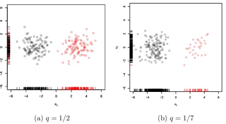
2.1 Bivariate data points generated from (2.11) with,q= 1/2,q= 1/7,
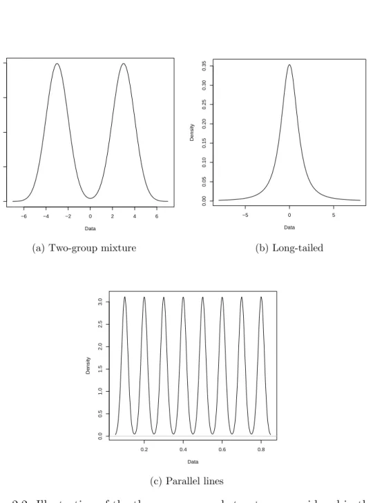
n= 200, α= 3, and a= (1,0)T. . . 23 2.2 Illustration of the three non-normal structures considered in the
thesis. . . 26
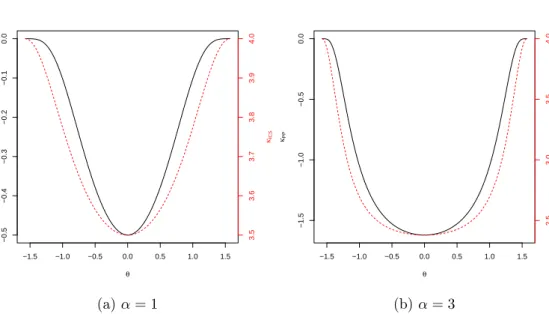
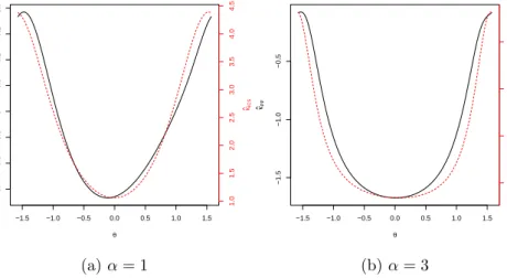
3.1 Plot of the population criteriaκICS(θ) (red dotted line), andκPP(θ)
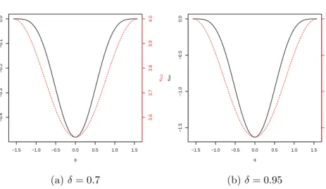
(solid black line) versusθ, for q= 1/2, α= 1, and 3. . . 46 3.2 Plot of the population criteriaκICS(φ) (red dotted line), andκPP(φ)
(solid black line) versusφ, forq = 1/2,δ = 0.7, and 0.95. . . 47 3.3 Plot of ˆκICS(θ) (red dotted line), and ˆκPP(θ) (solid black line)
ver-susθ, forq = 1/2, α= 1, and 3. . . 48 3.4 Plots of θ and φ, when c1 = 3, c2 = 1. . . 51
3.5 For α = 1,3 and q = 1/2, 1/4, the plots of ˆv(ˆθPP) (black solid
curves) and ˆv(ˆθICS) (red dashed curves). . . 55
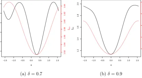
5.1 Plot of ICS criteria ˆκICS(θ) (red dotted line), and PP criteria ˆκPP(θ)
(solid black line) versusθ, for q= 1/2, δ= 0.7, and 0.9. . . 79 5.2 Histograms of 0◦,15◦,30◦ and 90◦ projections, with the vectors of
data contained in the shorh interval (the lower red lines), and in ¯
x±s interval the (upper blue lines). . . 82 5.3 Histograms of 0◦,15◦,30◦ and 90◦ projections, with shoth interval
List of Figures ix
5.4 The plot of ICS:variance:mve (red dashed curve) and PP(Mean):variance:lshorth (black solid curve) using a common mean ¯x. . . 85
5.5 The plot of ICS(MVE):t2M-estimate:MVE and PP(lshorth):t2
M-estimate:lshorth. . . 86
5.6 The plots of PPd:variance:lshorth (the black solid curve), and ICSd:variance:MVE (the red dashed curve). . . 87
5.7 The plots of PPd:t2M-estimate:lshorth (the black solid curve) and
ICSd:t
2M-estimate:MVE (the red dashed curve). . . 87
7.1 The scatter plot of RANDU data set (a) and the transformed data set (b). . . 116 7.2 The scatter plot of a subset of RANDU data set. . . 117 7.3 The histograms of θij. . . 119 7.4 The density plots of the projected normal density function gj(θ),
for |j|= 0.1,0.5,1,3. . . 128 7.5 Histograms ofθ of data points simulated fromN(0,1) lying on two
parallel lines separated by j = 0.1,0.5,1,3. . . 129 7.6 Histograms ofθ of data points simulated from C(0,1) lying on two
parallel lines separated by j = 0.5,2,4. . . 133
8.1 (a) Illustration of the algorithm withh= 0.2 and l = 0.2, and (b) the local means that form the principal curve. . . 141 8.2 Illustration of the solutions of the local PCA and ICS at a selected
iteration, for two parallel curves with step length l = 0.1, and radius h= 0.1. . . 143 8.3 A full fingerprint image of dimension 379×388. . . 144 8.4 A subset, of dimension 40×40, from the full fingerprint image that
shows the parallel ridges. . . 144 8.5 The direction of the smallest eigenvector of S−1Vˆ, for the parallel
List of Tables
4.1 The values of asymptotic variances of ˆφICSand ˆφPP, forδ= 0.1,0.5,0.7,0.9,1. 73
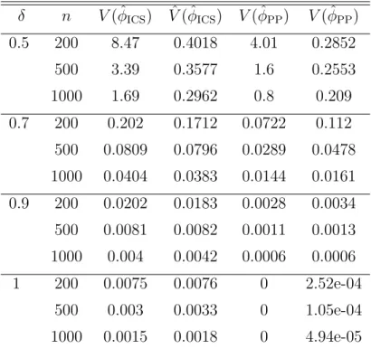
4.2 The sample variances and asymptotic variances of ˆφICS and ˆφPP,
for different δ and n . . . 74
6.1 Variances of different estimates ofθ, where the true signal direction isθ = 0◦. . . 111 6.2 Variances of different estimates ofθ, where the true signal direction
isθ = 45◦. . . 111 6.3 Variances of different estimates ofθ, where the true signal direction
isθ = 90◦. . . 111 6.4 Percentage of picking the right eigenvector. . . 111
7.1 The means of axis squared distance of the smallest eigenvector of ˆ
V for simulated bivariate data consists k = 10 parallel lines, with dimensions p= 2,3,4,6, and sample sizes 40p,160p,400p. . . 126 7.2 The accuracy of the estimate of ICSd:W-estimate:variance, for
Chapter 1
Introduction
The subject of this thesis is the invariant coordinate selection (ICS) method, de-veloped to discover structures in multivariate data using the eigenvalue-eigenvector decomposition of two different scatter matrices. The performance of the ICS method depends on the structure of the data and the pair of scatter matrices used.
The main goal of this thesis is to understand why ICS works in some situations, and not others. Another goal is to compare ICS to the projection pursuit method (PP).
The general tools used in this thesis are multivariate analysis and robust statistics. We start by giving a brief introduction of these two topics.
1.1
Multivariate analysis
Multivariate analysis is concerned with the analysis of data of dimensionphigher than one. References in multivariate analysis include Mardia et al. (1980), and Everitt (2005).
A p-dimensional dataset, with n observations can be represented by ann×p
data matrix, X, say. Each row is denoted by xT
Chapter 1. Introduction 2
matrix X can be written in terms of its rows as
X = xT 1 .. . xT n , where xTi = (xi1, . . . , xip).
1.1.1
Transformations
As a preliminary step of the analysis, multivariate data can be transformed using one of the following transformations:
(1) Non-singular transformation: for a non-singular p×p matrix, Q, say, and a vector b ∈Rp, suppose that X is transformed as follows
X →XQT + 1nbT, (1.1)
where 1n is a vector of lengthn with all its components equal to one. Standardization is an example of affine transformation. In standardization, each row ofXis shifted to have zero mean, and scaled to have unit variance,
X →(X−1nx¯)S−1/2,
where ¯xis the mean vector, defined in (1.5), andS−1/2 is the inverse square
root of the sample covariance matrix S, defined in (1.8), and (1.6), respec-tively. Standardization removes the correlation effect between variables, and scale the variance of each variable to 1. In this case the covariance matrix of the standardized data is equal to the identity matrix.
Chapter 1. Introduction 3
aj 6= 0, j = 1, . . . , p. Suppose thatX is transformed as follows:
X →XA. (1.2)
For example, if the components of X are measured in different scales, we can unify the measurement scales by choosing A as diag(1/sjj), where sjj is the standard deviation of the jth component of X, j = 1, . . . , p.
(3) Orthogonal rotation: LetR be ap×protation matrix, such thatRTR=I p, and |R|= 1. A rotation ofX is defined as
X →XRT. (1.3)
The two dimensional rotation matrix is equal to
R = cos(ω) −sin(ω) sin(ω) cos(ω) . (1.4)
It is often important that multivariate techniques are affine equivariant. A mul-tivariate technique is said to be affine equivariant if under any of transformations (1), (2), and (3), the results of the analysis are not affected. As we have mentioned earlier, if the scales of the measurements are unified, or the data is standardized, it is desirable that the performance of method is not affected by the transformation. Methods that are equivariant under non-singular transformations in (1) are preferable. Most methods are equivariant under at least one of the transforma-tions (1), (2) or (3).
For example, Mahalanobis distances, and linear discriminant analysis are equivariant methods under non-singular transformations. Factor analysis is equiv-ariant under scale change transformation in (2). PCA is equivequiv-ariant under or-thogonal transformations.
Chapter 1. Introduction 4
1.1.2
Summary statistics
The sample mean vector is defined as
¯
x= 1
nX
T1
n. (1.5)
The sample covariance matrix is defined as
S= 1
n(X−1nx¯
T)T(X−1
nx¯T). (1.6)
The spectral decomposition of S is given by
S =U LUT, (1.7)
whereL=diag(l1, . . . , lp) is a diagonal matrix containing the ordered eigenvalues, and U = (u1, . . . , up) is a p×p matrix whose its columns are the corresponding eigenvectors.
The inverse square root of S can be defied as follows
S−1/2 =U L−1/2UT, (1.8) where L−1/2 =diag(l1−1/2, . . . , l−p1/2).
The sample mean and the sample covariance matrix are affine equivariant under linear transformations. Consider the non-singular transformation in (1.1). The sample mean and covariance matrix are given by
¯
x→Qx¯+b, S→QSQT.
Chapter 1. Introduction 5
1.1.3
Exploratory data analysis
Usually, the first step of the analysis is to explore the multivariate data. Ex-ploratory analysis helps to
• choose appropriate models by detecting departure from normality, including groups, and outliers;
• reduce the dimension of the data by assessing the linear relationships be-tween variables.
In the following we define some of the classical methods that can be used to explore multivariate data.
Principal component analysis
Principal component analysis finds the linear combination for which the data have maximal variance. The aim is to reduce the dimension, and understand the covariance structure of the data.
Consider the linear transformation Xa, where a ∈ Rp is a unit vector. The mean of Xa is equal toaTx¯, and the variance is equal to aTSa.
PCA reduces the dimension by projecting the data onto the subspace spanned by the k eigenvectors corresponding to the k < p largest eigenvalues,
Y = (X−1nx¯T)V,
where V is a p ×k matrix, its columns are the k largest eigenvectors. The dimension of the reduced dataset Y is n×k.
Factor analysis
In Factor analysis it is assumed that each measurement depends on unobservable common factors. The goal is to find the linear relationship between the
com-Chapter 1. Introduction 6
mon factors and the measurements. This relationship can be used to reduce the dimension of the data.
In a factor model, a p-variate random vector is written as the sum of a linear combination of k < p dimension vector of common factors plus unique factors. Let xbe a p-variate random vector, the factor model is given by
x= Λf+u,
where Λ is a p×k (k < p), matrix of constants, f is a k×1 vector of common factors, and u is a p×1 vector of unique factors.
The model assumptions are
E(x) = E(f) = 0,var(f) = Ik,
E(u) = 0,var(u) = Ψ = diag(ψ1, . . . , ψp),cov(f, u) = 0. Thus, the covariance matrix can written as
Σ = ΛΛT + Ψ, where σii = k X j=1 λ2ij +ψi. (1.9)
This means that the variance of each variable can be divided into two parts: the communalities, h2i = k X j=1 λ2ij,
and the unique variance ψi.
Given multivariate data, there are two methods to estimate Λ and Ψ: the first is the principal factor analysis and the second is the maximum likelihood method, where the common factors and unique factors are assumed to be normally
Chapter 1. Introduction 7
distributed. We explain briefly the first method in the following paragraph. Since the factor model is equivariant under the change of scale, as in (1.2), the variables can be scaled to have unit variances. Hence, the covariance matrix of the scaled data is equal to the correlation matrix ˆR.
The method is based on finding the reduced correlation matrix as follows
ˆ
R−Ψ = ˆˆ Λ ˆΛT.
We need first to estimate the cummunalitesh2i, which can be estimated iteratively using the previous equation and the following equation, from (1.9),
ˆ
ψi = 1−h2i. The spectral decomposition of ˆR−Ψ is given byˆ
ˆ R−Ψ =ˆ p X i=1 aiγiγiT,
where a1 ≥ . . . ≥ ap are the eigenvalues of ˆR−ψˆ, and ˆγ1, . . . ,ˆγp are the corre-sponding eigenvectors.
The k eigenvectors corresponding to the largest k eigenvalues can be used as an estimate of Λ.
1.2
Location vectors and Scatter matrices
A vector-valued function T(X)∈Rp is a location vector if it is equivariant under affine transformations, which is defined in (1.1), as follows
Chapter 1. Introduction 8
A matrix-valued function S(X) is a scatter matrix if it is positive definite p×p
symmetric matrix, and affine equivariant
S(X)→QS(X)QT.
1.3
Robust statistics
Many statistical methods rely on the normality assumption of the data. In prac-tice, however, the normality assumption holds at best approximately. This means that the model describes the majority of the data, but a small proportion of the data do not fit into this model. This kind of atypical data are called outliers. Outliers are not always bad data, but may contain significant information.
Using classical statistical methods in the presence of outliers would give un-reliable results. Many robust statistical methods have been developed to tackle this problem. Maronna et al. (2006) and Jureckova and Picek (2005) are general references in robust statistics.
Maronna et al. (2006), page xvi, gives the following definition of robust meth-ods:
The robust approach to statistical modeling and data analysis aims at deriving methods that produce reliable parameter estimates and associated tests and confidence intervals, not only when the data fol-low a given distribution exactly, but also when this happens approxi-mately. . . .
1.3.1
Measuring robustness
Letx1, . . . , xn be an independent identically distributed replicate of a univariate random variablex. LetF(x;ϕ) be the distribution function ofx, whereϕ=T(x)
Chapter 1. Introduction 9
is an unknown parameter. The parameter ϕcan be written as a functional
ϕ=T(F).
An estimator of ˆϕn =T(x1, . . . , xn), can be written as ˆ
ϕn=T(Fn),
where Fn is the empirical distribution function defined as follows
Fn(t) = 1 n n X i=1 I(xi ≤t),
where I(A) is the indicator random variable which equals 1 when A holds. The -contamination distribution is defined as follows,
F = (1−)F +δx◦, (1.10)
where 0≤ ≤1, δx◦ is the point mass distribution where Pr(x=x◦) = 1.
Sensitivity curve
The effect of on the estimator ˆϕn = T(x1, . . . , xn) adding a new observation x◦
can be measured by the difference
SC(x◦;T, Fn) =T(x1, . . . , xn, x◦)−T(x1, . . . , xn) =T(Fn+1)−T(Fn).
The empirical distribution function of the contaminated sampleFn+1 is given by
Fn+1(t) = 1 n+ 1( n X i=1 I(xi ≤t) +I(x◦ ≤t)) = n n+ 1Fn+ 1 n+ 1δx◦.
Chapter 1. Introduction 10
Hence the sensitivity curve is defined by
SC(x◦;T, Fn) =T[
n
n+ 1Fn+ 1
n+ 1δx◦]−T(Fn). (1.11)
For example, the sample mean ˆϕn=T(Fn) is defined as
ˆ ϕn =T(Fn) = Z xdFn= Pn i=1xi n = ¯x. Define ˆϕn+1 =T(Fn+1) as follows ˆ ϕn+1 =T(Fn+1) = n n+ 1x¯+ 1 n+ 1x◦. The sensitivity curve is given by
SC(x◦;T, Fn) = n ( n n+ 1)¯x+ ( 1 n+ 1)x◦ −x¯ o = 1 n+ 1(x◦−x¯).
From the sensitivity curve of ¯x, as the value of the outlier x◦ increases, the
sensitivity curve becomes unbounded.
Influence function
The influence function for an estimator ˆϕn =T(Fn) is the population version of its sensitivity curve. To derive the influence function, consider the contaminated distribution in (1.10). The influence function is defined as
IF(x0;T, F) = lim →0 T ((1−)F +δx0)−T(F) = ∂ ∂ T ((1−)F +δx0)|=0 . (1.12) For example, the expected value as the parameter of interest: ϕ = T(F) =
Chapter 1. Introduction 11
E(X). Then,
T(F) =T ((1−)F +δx0) = (1−)T(F) + T(δx0)
= (1−)E(X) + x0.
The influence function of the expected value is
IF(x0;T, F) = lim →0 (1−)E(X) + x0−E(X) =x0−E(X). Breakdown point
The breakdown point of an estimator ˆϕ = T(x1, . . . , xn) is the largest possible fraction of contamination such that the estimator remains bounded.
An estimator with a high breakdown point means it is a robust estimator. For example the breakdown point of the mean is 0, since changing a single observation may increase the mean without bound, while the for the median is equal to 1/2.
1.3.2
Robust location and scale estimates
If the data are normally distributed, then the sample mean and the sample vari-ance are the optimal location and scale estimates. Since we only knowF approx-imately, we want the estimates of location and scale to be reliable in the presence of outliers.
In the following we discuss briefly some of robust location and scale estimates. We consider first univariate estimates. After that, we discuss the multivariate analogues of some of the univariate estimates discussed in this section.
Univariate estimates
The simplest alternative to the sample mean is the median (Med); alternatives to the sample variance include the interquartile range (IQR) and mean absolute
Chapter 1. Introduction 12
deviation (MAD).
In the following, we define the univariate robust estimates that are used in this thesis.
• M-estimate: Suppose that ϕ = (µ, σ2). The M-estimates of location and scale are the solutions of the following estimation equations
ˆ µ= Pn i=1w1(ri)xi Pn i=1w1(ri) , σˆ2 = Pn i=1w2(ri) n , (1.13)
where w1 and w2 are non-negative weight functions, and
ri =
xi−µˆ ˆ
σ .
For example, the maximum likelihood estimate of tν-distribution have the following weight functions
w1(ri) =w2(r1) = (ν+ 1)/(ν+r2).
Equations (1.13) are solved iteratively, i.e we start by assigning initial values to ˆµ and ˆσ2 to compute the weights. Then we can solve equations (1.13)
iteratively, update the weights in each iteration, until convergence.
• The lshorth: The lshorth is defined as the length of the shortest interval that contains half of observations. Its associated location measure is the midpoint of the shortest interval (shorth).
The shorth was first introduced by Andrews et al. (1972) as the mean of data points in the shortest interval which contains half of observations. An-drews et al. (1972) showed that the mean of the shorth has bad asymptotic performance, its limiting distribution is not normal, and its rate of conver-gence is of order n−3. Grubel (1988) suggested the use of the shorth as a
Chapter 1. Introduction 13
scale measure, lshorth. The lshorth is defined as follows
ln(x1, . . . , xn) = min{x(i+j)−x(i) : 1≤i≤i+j ≤n,(i+j)/n≥1/2}.
(1.14)
Multivariate estimates
• M-estimate: The multivariate M-estimate of location and scale are the solution of the following two equations:
ˆ µ= Pn i=1w1(ri)xi Pn i=1w1(ri) , ˆ Σ = Pn i=1w2(ri)(xi−µˆ)(xi−µˆ) T n , (1.15) where ri = (xi −µˆ)TΣ(ˆ xi−µˆ).
• The minimum volume ellipsoid (MVE): The minimum volume ellipsoid, Van Aelst and Rousseeuw (2009), is defined as the smallest ellipsoid con-taining at least half of observations. The MVE is the multivariate version of the lshorth. Like the lshorth, MVE has a high breakdown point, but bad asymptotic behavior with n−1/3 rate of convergence. In practice, MVE is
computationally expensive.
1.4
Thesis outline
When investigating ICS and PP, we need to specify: • pair of spread measures;
• structure of the data;
• The computation of the measures of spread: based on the associated lo-cation measures, based on a common lolo-cation measure, or based on the
Chapter 1. Introduction 14
pairwise differencing of the data to force the symmetry of the data around the origin.
In Chapter 2, we explore the rationale of the ICS method. We also link PP to ICS.
In Chapter 3, we explore the ICS criterion based on the fourth-order moment matrix and the covariance matrix and the PP based on kurtosis, under two-group mixtures of bivariate normal distributions. We also compare the accuracy of the two methods through a simulation study.
Under equal mixtures of two bivariate normal distributions, we derive the asymptotic distributions of the ICS and PP estimates of the group separation direction in Chapter 4.
ICS and PP kurtosis criteria are not robust, in the sense that they are highly affected by outliers. Both ICS and PP criteria can be defined based on two robust measures of scale. In Chapter 5, we investigate the feasibility of using robust measures of spread in ICS and PP. We also explore the effect of using a common location measure in the measures of spread used in ICS and PP criteria, and the role of pairwise differencing of data.
The errors in variables model, EIV, is a regression model with both mea-surements are subject to errors. In Chapter 6 we explore using ICS based on the fourth-order moment matrix and the variance in fitting EIV line. We also compare the ICS method to Geary’s fourth-order cumulant-based estimators.
The performance of ICS depends on the choice of the pair of scatter matrices, and the structure of the data at hand. For example, ICS based on the fourth-order moment matrix is not able to find the structure direction in the RANDU data set. The points in the RANDU data set are arranged on 15 parallel planes, lying in three dimensional space. The structure direction in the RANDU data set is the direction that views the parallel line structure. In Chapter 7, we explore the choice of the two scatter matrices in ICS that can find such the parallel line structure in such data. Namely, the W-estimate and the covariance matrix. We
Chapter 1. Introduction 15
also explore the effect of using the pairwise differencing of the data in W-estimate. Two potential applications of ICS are discussed in Chapter 8. We discuss the role ICS can play in finding principal curves and in the analysis of fingerprint images.
Chapter 2
Invariant coordinate selection
and related methods
2.1
Introduction
Suppose we have a multivariate data set that has a lower dimensional struc-ture. One way to detect structure is by projecting the data onto a line for which the data is maximally non-normal. Hence, methods that are sensitive to non-normality can be used to detect structure. Two such methods from the lit-erature: invariant coordinate selection (ICS), introduced by Tyler et al. (2009), and projection pursuit(PP), introduced by Friedman and Tukey (1974).
ICS and PP find structure direction by optimizing criteria sensitive to non-normality. Any summary statistic that is sensitive to non-normality can be used as a criterion. For example, the univariate kurtosis is zero when a random variable has normal distribution. For normal distributions the kurtosis is mostly non-zero, positive or negative.
Motivated by kurtosis, the ICS and PP optimality criteria can be defined as ratios of any two measures of spread.
The structure of this chapter is as follows. In Section 2.2, we explore the rationale of the ICS method. After that we link the ideas of ICS to PP in Section
Chapter 2. Invariant coordinate selections and related methods 17
2.3. In Section 2.4, the use of kurtosis as a criterion to identify non-normal directions of the data is reviewed. In Section 2.5, the idea of using a common location measure in the calculations of the pair of spread measures in ICS and PP is introduced. In Section 2.6, the role of differencing on ICS and PP is discussed. In Section 2.7, we go through non-normal structures, considered in this thesis, and their corresponding models. In Section 2.8, we discuss how to choose the pair of spread measures for ICS and PP. Notations are introduced in Section 2.9.
2.2
Rationale of the invariant coordinate
selec-tion method
LetX be ann×pdata matrix, where its rows arexTi = (xi1, . . . , xip),i= 1, . . . , n. ICS finds a direction a ∈ Rp for which Xa is maximally non-normal, using the relative eigenvalue-eigenvector decomposition of two affine equivariant scatter matrices with different level of robustness.
Let S1 = S1(X) and S2 =S2(X), be two affine equivariant scatter matrices.
Each scatter matrix is associated with a location measure, ˆµ1 = ˆµ1(X) and
ˆ
µ2 = ˆµ2(X), say.
The ICS criterion, based on S1 and S2, is to find a direction a that
mini-mizes/maximizes the following criteria
ˆ κICS(a) = aTS 1a aTS 2a . (2.1)
The minimum/maximum value of (2.1) is the smallest/largest eigenvalue ofS2−1S1,
obtained when a is the corresponding eigenvector.
An eigenvalue λ and eigenvector a of S2−1S1 are the solution of the following
equation
Chapter 2. Invariant coordinate selections and related methods 18
Suppose that X is transformed by the affine transformation in (1.1). Denote the transformed data matrix by X∗. Then, the scatter matrices S1∗ = S1(X∗),
and S2∗ =S2(X∗) become
S1∗ =QS1QT
S2∗ =QS2QT,
since S1(·) and S2(·) are affine equivariant.
Let
b=Q−Ta. (2.3)
The eigenvalues and eigenvectors ofS2∗−1S1∗ are the solution of the following equa-tion S2∗−1S1∗b =Q−TS2−1Q−1QS1QTQ−Ta =Q−TS2−1S1a. From (2.2), S2∗−1S1∗b=Q−Tλa =λb. (2.4)
From (2.2) and (2.4), the eigenvalues ofS2∗−1S1∗ andS2−1S1 are the same, whereas
the eigenvectors ofS2∗−1S1∗ are the eigenvectors of S2−1S1 scaled by Q−T.
The PCA can be related to (2.2), with S2 taken as the identity matrix. Since
ICS is affine equivariant, as we have shown earlier in (2.2) to (2.4), we may standardize X with respect to Q = S2−1/2, such that S2∗ = Ip. In this case, ICS can be seen as applying the PCA of the standardized dataX∗ with respect toS1∗.
Chapter 2. Invariant coordinate selections and related methods 19
2.3
Projection pursuit as a variant of invariant
coordinate selections
As ICS, PP finds a direction a, such that the projection Xa is maximally non-normal. The PP criterion can be defined as a ratio of two univariate affine equivariant measures of scale, s1 and s2, say:
κPP(a) =
s1(Xa)
s2(Xa)
. (2.5)
In contrast to ICS, minimizing/maximizing (2.5) is computationally expensive because it is carried out numerically. PP method searches in all projection direc-tions to find the direction that minimizing/maximizing (2.5).
Suppose that X is standardized as in (1.1). Criterion (2.5) based on the standardized data X∗ becomes
κPP(b) =
s1(X∗b)
s2(X∗b)
. (2.6)
Where b is as in (2.3), and can be noted by comparing the following two linear transformations,
Xa∝X∗b
=XQTQ−Ta. (2.7)
We explore the effect of standardization on PP in Section 3.6.
2.4
Univariate kurtosis
The kurtosis of a univariate random variable u, say, is defined as follows.
kurt(u) = E{(u−µu)
4}
[E{(u−µu)2}]
Chapter 2. Invariant coordinate selections and related methods 20
where µu, is the mean value of u.
The kurtosis takes the following possible values:
(1) kurt(u) = 0: satisfied under normality.
(2) kurt(u)<0: this case is called sub-Gaussian.
(3) kurt(u)>0: this case is called super-Gaussian.
The Sub-Gaussian case appears in distributions flatter than the normal and have thinner tails; examples include the uniform distribution. On the other hand, the super-Gaussian case appears in distributions that are more peaked than the normal distribution and have longer tails; examples include t, and Laplace distri-butions.
The extreme case of sub-Gaussianity occurs for two-point distribution. That is, letsbe a random variable that has a two-point distribution, defined as follows.
s= 1 with probability q −1 with probability (1−q) . (2.9)
The kurtosis of s is equal to
kurt(s) = −3[4q(1−q)]
2+ 16q(1−q)
(4q(1−q))2 −3
= 1
q(1−q)−6. (2.10)
The minimum value of kurt(s) is−2, attained whenq = 1/2. The value of kurt(s) increases as q increases away from 1/2, as shown in the following lemma.
Lemma 2.4.1. The kurtosis of any random variable takes the values between −2
and ∞.
Proof. This lemma can be proved using the Cauchy-Schwarz inequality. The Cauchy-Schwarz inequality for a random variable u, where E(u) = 0, is given as
Chapter 2. Invariant coordinate selections and related methods 21
follows
(E{u2})2 ≤E{u4}.
Dividing both sides by (E{u2})2 and subtracting 3
E{u4}
(E{u2})2 −3≥1−3
kurt(u)≥ −2.
The kurtosis has been used as a criterion for identifying non-normal projec-tions of multivariate data in PP and independent component analysis (ICA); see for example, Huber (1985), Jones and Sibson (1987), Pe˜na and Prieto (2001), and Bugrien and Kent (2005).
Pe˜na and Prieto (2001) suggested that minimizing kurtosis is appropriate if the purpose is identifying clusters, whereas maximizing kurtosis can be used to detect outliers. In particular, if q is near half, minimizing kurtosis is more useful than maximizing it; if q is far from half maximizing kurtosis is more useful than minimizing it. Pe˜na and Prieto (2001) also gave a threshold ofqthat distinguishes
q from being far from half or near half. The threshold can be noted from (2.9). Namely, if q(1−q) = 1/6 the kurtosis equals to zero, otherwise the kurtosis will be negative or positive.
To illustrate the idea of minimizing and maximizing kurtosis, consider n bi-variate data points generated by adding a bibi-variate isotropic noise to points gen-erated fromsin (2.9). That is, the data pointsxiare generated from the following model xi =si α 0 +i, (2.11)
Chapter 2. Invariant coordinate selections and related methods 22
a bivariate normal isotropic noise. The structure direction in this model is the direction that best separate the two groups, at the horizontal direction, and the noise direction is in the direction the data are normally distributed, the vertical direction, as shown in Figures 2.1(a) and (b), with q= 1/2 and 1/7, andα = 3.
Chapter 2. Invariant coordinate selections and related methods 23 ●● ● ● ● ● ● ● ● ● ● ● ● ● ● ● ● ● ● ● ● ● ● ● ● ● ● ● ● ● ● ● ● ● ● ● ● ● ● ● ● ● ● ● ● ● ● ● ● ● ● ● ● ● ● ● ● ● ● ● ● ● ● ● ● ● ● ● ● ● ● ● ● ● ● ● ● ● ● ● ● ● ● ● ● ● ● ●● ● ● ● ● ● ● ● ● ● ● ● −6 −4 −2 0 2 4 6 −6 −4 −2 0 2 4 6 x1 x2 ● ● ● ● ● ● ● ● ● ● ● ● ● ● ● ● ● ● ● ● ● ● ● ● ● ● ● ● ● ● ● ● ● ● ● ● ● ● ● ● ● ● ● ● ● ● ● ● ● ● ● ● ● ● ●● ● ● ● ● ● ● ● ● ● ● ● ● ● ● ● ● ● ● ● ● ● ● ● ●● ● ● ● ● ● ● ● ● ● ● ● ● ● ● ● ● ● ● ● −6 −4 −2 0 2 4 6 −6 −4 −2 0 2 4 6 x1 x2 (a)q= 1/2 ● ● ● ● ● ● ● ● ● ● ● ● ● ● ● ● ● ● ● ● ● ● ● ● ● ● ● ● ● −6 −4 −2 0 2 4 6 −6 −4 −2 0 2 4 6 x1 x2 ● ● ● ● ● ● ● ● ● ● ● ● ● ● ● ● ● ● ● ● ● ● ● ● ● ● ● ● ● ● ● ● ● ● ● ● ● ● ● ● ● ● ● ● ● ● ● ● ● ● ● ● ● ● ● ● ● ● ● ● ● ● ● ● ● ● ● ● ● ● ● ● ● ● ● ● ● ● ● ● ● ● ● ● ● ● ● ● ● ● ● ● ● ● ● ● ● ● ● ● ● ● ● ● ● ● ● ● ● ● ● ● ● ● ● ● ● ● ● ● ● ● ● ● ● ● ● ● ● ● ● ● ● ● ● ● ● ● ● ● ● ● −6 −4 −2 0 2 4 6 −6 −4 −2 0 2 4 6 x1 x2 (b)q= 1/7
Figure 2.1: Bivariate data points generated from (2.11) with, q = 1/2, q = 1/7,
n = 200,α = 3, and a= (1,0)T.
In (a), the value of the sample kurtosis in the horizontal direction is −1.7, while in the vertical is 0.2. In (b), the sample kurtosis in the horizontal direction is 1.3, while in the vertical direction is −0.8.
The structure direction is in the direction that minimizes or maximizes the kurtosis relative to the kurtosis of the data in the noise direction.
2.5
Common location measure
The computation of each measure of spread in criterion (2.1) and (2.6) is based on an associated location measure. Sometimes different location measures are used in the denominator and numerator, which makes the methods unreliable.
One possible way to solve this problem is by using a common location measure in the denominator and numerator. Another way is by computing the scale measures based on pairwise differencing of the data to force the symmetry of the data around the origin. The pairwise differencing of the data is defined in the following section. This problem is explored in Chapter 5.
Chapter 2. Invariant coordinate selections and related methods 24
2.6
Role of differencing
Let X be an n×p data matrix, with its rows xTi = (xi1, . . . , xip), i = 1, . . . , n. The pairwise differencing of X, denoted byXd, is defined as follows,
xdk=xi−xj, i6=j = 1, . . . , n, (2.12)
where k = 1, . . . , n(n−1).
As we noted earlier in Section 2.5, pairwise differencing can be used to force the symmetry of the data around the origin.
Another problem that involves differencing of the data is when the structure is similar to the RANDU example from Tyler et al. (2009). The data points in RANDU data set, explained in Section 7.2, are arranged in 15 parallel planes, evenly spaced. The structure direction in this data set is the direction that views the parallel lines structure.
The pairwise differences of RANDU-like data produce inliers. Inlers are points with small lengths, arise as a result of the difference of two points with small distance.
A sensible choice of the pair of scatter matrices for such data should accen-tuates inliers to emphasize the parallel line structures. Chapter 7 discusses the choice of the pair of scatter matrices in this kind of structure.
2.7
Types of non-normal structures
Examples of departure from non-normality include skewed, long-tailed, and mix-ture distributions. The focus in this thesis will be on the following non-normal structures:
(I) Two-group mixtures: this structure is defined in Section 3.2. Figure 2.2 (a) shows plot the two-group structure.
Chapter 2. Invariant coordinate selections and related methods 25
(II) Long-tailed: this structure can be defined by the errors-in-variables model in Section 6.2, when the signal has non-normal distribution. The long-tailed structure is shown in Figure 2.2 (b).
(III) Parallel lines structure: this structure is defined in the RANDU-type model defined in Section 7.3. The parallel line structure is shown in Figure 2.2 (c).
2.8
How to choose the pair of scatter matrices
In this Section, we largely follow the classification of scatter matrices from Tyler et al. (2009), who divided the scatter matrices into three classes. We have added a new class, Class I. The classes of scatter matrices are given as follows:
• Class I is the class of highly non-robust scatter matrices, with zero break-down point and unbounded influence function. The scatter matrices in-cluded in this class are highly affected by inliers or outliers. Examples include weighted scatter matrices that up-weight outliers, or inliers, such as the fourth-order scatter matrix ˆK, defined in (3.23), and the one-step W-estimate ˆV, defined in (7.1).
• Class II is the class of non-robust scatter matrices with zero breakdown points and unbounded influence function. Examples include the covariance matrix.
• Class III is the class of scatter matrices that are locally robust, in the sense that they have bounded influence function and positive breakdown points not greater than p+11 . An example from this class is the class of multivariate M-estimators, e.g M-estimate for t-distribution, Arslan et al. (1995).
• Class IV is the class of scatter matrices with high breakdown points such as the Stahel-Donoho estimate, the minimum volume ellipsoid, Van Aelst
Chapter 2. Invariant coordinate selections and related methods 26 −6 −4 −2 0 2 4 6 0.00 0.05 0.10 0.15 0.20 Data Density
(a) Two-group mixture
−5 0 5 0.00 0.05 0.10 0.15 0.20 0.25 0.30 0.35 Data Density (b) Long-tailed 0.2 0.4 0.6 0.8 0.0 0.5 1.0 1.5 2.0 2.5 3.0 Data Density (c) Parallel lines
Figure 2.2: Illustration of the three non-normal structures considered in the the-sis.
Chapter 2. Invariant coordinate selections and related methods 27
and Rousseeuw (2009) and the constrained M-estimates, Kent and Tyler (1996).
Motivated by the univariate kurtosis, the ICS pair of scatter matrices can be chosen from different classes. By convention, the scatter matrix in the denomi-nator is more robust that the one in the numerator.
In the following, we list the scatter matrices that are used in ICS:
1. The fourth-order moment matrix, defined in (3.23).
2. The covariance matrix, defined in (1.6).
3. The M-estimator fort2 distribution, defined in Section 1.3.2.
4. The minimum volume ellipsoid, defined in Section 1.3.2.
5. The one-step wighted scatter matrix , defined in (7.1), usually computed based on pairwise differencing.
Similarly, in PP the univariate analogues of some of the scatter matrices, listed above, are used,
1. The univariate kurtosis, defined in (2.8).
2. The variance.
3. The univariate M-estimate for t2 distribution, defined in (1.13).
4. The lshorth, defined in (1.14).
2.9
Notation
Throughout the thesis the following notation will be used:
• Univariate random variables and multivariate random vectors, and their realizations, are denoted by small letters, x, say.
Chapter 2. Invariant coordinate selections and related methods 28
• Data matrices will be denoted by capital letters, X, say.
• The notations of ICS and PP methods are as follows:
– ICS and PP, based on two different measures of scales, computed with respect to the associated location measures, are denoted by
ICS : Spread 1 : Spread 2,
PP : Spread 1 : Spread 2.
For example, ICS and PP based on kurtosis and variance are denoted by
ICS : kurtosis : variance,
PP : kurtosis : variance.
– ICS and PP with respect to a common location measure will be de-noted by
ICS(Location) : Spread 1 : Spread 2,
PP(Location) : Spread 1 : Spread 2.
– ICS and PP with respect to differenced data are given the superscript
d, i.e
ICSd: Spread 1 : Spread 2,
PPd: Spread 1 : Spread 2.
• The ICS criterion based on any pair of scatter matrices will be denoted by: inp-dimensionκICS(a), as function of the unit vectora∈Rp; two-dimension
Chapter 2. Invariant coordinate selections and related methods 29
• Similarly, PP criterion is denoted by κPP(a) in p-dimension, and κPP(θ) in
Chapter 3
Using ICS and PP based on
fourth-order moments in
two-group mixtures
3.1
Introduction
In this chapter we explore the theory and practice of ICS:kurtosis:variance and PP:kurtosis:variance, under mixtures of two bivariate normal distributions. The ICS and PP methods are defined in Sections 2.2 and 2.3. The main goal is to compare the accuracy of ICS and PP in identifying the group separation direction. The structure of this chapter is given as follows. In section 3.2, we define the model, mixtures of two bivariate normal distributions. In Section 3.3 we discuss the theory of ICS:kurtosis:variance. In Section 3.4, the relationship between Mardia’s multivariate measure of kurtosis and ICS:kurtosis:variance. In Section 3.5, the theory of PP:kurtosis:variance under the mixture model is discussed. In Section 3.6, we define ICS:kurtosis:variance, and PP:kurtosis:variance criteria in population and sample cases. We define a measure of spread between axes in Section 3.7, that is used to compare the accuracy of the two methods. In Section 3.8, a simulation study is conducted to compare ICS and PP.
Chapter 3. Using ICS and PP based on fourth-order moments in
two-group mixtures 31
3.2
The model: Mixtures of two bivariate
nor-mal distributions
3.2.1
The model assumptions
Let z = (z1, z2)T be a bivariate random vector, with mean µ and covariance
matrix Σz, distributed as a mixture of two bivariate normal distributions, with mixing proportion q.
Assume for simplicity that the two groups have equal within-group covariance matrices, Wz. The density function of z is given by
f(z) =qg(z;µ1, Wz) + (1−q)g(z, µ2, Wz). (3.1) where µ1 and µ2 are the group mean vectors, and g is the marginal normal
distribution given by g(z;µi, Wz) =|2πWz|−1/2exp{− 1 2(z−µi) TW−1 z (z−µi)}. where |Wz|>0.
Since ICS and PP are equivariant methods, under translation, rotation, and affine transformations, we may, without loss of generality, assume the following
(1) The random vector z is translated and rotated such that the group means lie on the horizontal direction, and become symmetric around the origin,
z0 =Rz,
Chapter 3. Using ICS and PP based on fourth-order moments in
two-group mixtures 32
matrix and the total covariance matrix of z0 are
Wz0 =RWzRT,
Σz0 =RΣzRT.
(2) The random vectorz0 is standardized in either of two ways: with respect to
Wz0; or with respect to Σ
z0. Each standardization method gives a different coordinate system, as shown in the following.
(i) Suppose that z0 is standardized with respect to Wz0, as follows:
x=W−1/2
z0 z
0
. (3.2)
The group means are given by
µ1 = (α,0)T, µ2 = (−α,0)T, (3.3)
where the parameter α ≥ 0 is used here as a separation parameter between the group means. If α = 0, the distribution of x will be normal, and as α increases the groups become more separated.
The total mean vector is given by
µx =qµ1+ (1−q)µ2 = ((2q−1)α,0)T. (3.4)
The total covariance matrix is given by
Chapter 3. Using ICS and PP based on fourth-order moments in
two-group mixtures 33
whereBx is the between-group scatter matrix,
Bx =q(µ1−µx)(µ1−µx)T + (1−q)(µ2−µx)(µ2−µx)T = 4q(1−q)α2 0 0 0 . (3.6) Substituting (3.6) in (3.5) gives Σx = 1 + 4q(1−q)α2 0 0 1 . (3.7)
The standardized random vector x = (x1, x2)T can be written as
fol-lows x1 x2 =s α 0 + 1 2 . (3.8)
where= (1, 2)T is a normally distributed random vector, with zero
mean vector and covariance matrixWx =I2, and the random variable
s has a two-point distribution, defined in (2.9).
(ii) Suppose that z0 is standardized with respect to Σz0, as follows:
y= Σ−1/2 z0 z
0
. (3.9)
The group means are given by
µ1 = (δ,0)T, µ2 = (−δ,0)T,
where 0≤δ≤1. The total mean vector is given by
Chapter 3. Using ICS and PP based on fourth-order moments in
two-group mixtures 34
The between-group variance is given by
By = 4q(1−q)δ2 0 0 0 . (3.11)
The within-group variance Wy is equal to
Wy =I2−By = 1−4q(1−q)δ2 0 0 1 . (3.12)
The standardized random vectory= (y1, y2)T can be written as
y1 y2 =s δ 0 + ∗1 ∗2 . (3.13)
where∗ = (∗1, ∗2)T is a normally distributed random vector, with zero mean vector and covariance matrixWy, and the random variableshas a two-point distribution, defined in (2.9).
3.2.2
Univariate moments
In this section, we derive the univariate moments of the components of x, x1, x2,
and the components of y,y1, y2, up to fourth order, to use them in the derivation
of ICS:kurtosis:variance and PP:kurtosis:variance criteria in Sections 3.3 and 3.4. Let the rth-order non-central moment of a univariate random variableu, say, be denoted by µ0u(r), and the rth order central moment be denoted by µu(r), defined as follows, respectively
µ0u(r) = E{ur},
Chapter 3. Using ICS and PP based on fourth-order moments in
two-group mixtures 35
Let the (h+j)-order non-central cross moment of a bivariate random variable
u= (u1, u2)T, say, be denoted by µ
0
u1u2(h, j), and the (h+j) central order cross
moment about the mean vector be denoted by µu1u2(h, j), defined as follows,
respectively, µu1u2(h, j) = E{u h 1u j 2}, µu1u2(h, j) = E{(u1−µ 0 u1(1)) h(u 2 −µ 0 u2(1)) j}. (3.15)
If u1 and u2 are independent,µu1u2(h, j) =µu1(h)µu2(j).
From (3.8), the components of x are independent; the first component is distributed as a mixture of two normal distributions,
x1 ∼qN(α,1) + (1−q)N(−α,1),
and the second component is distributed as N(0,1). Similarly, from (3.13), the first component of y is distributed as
y1 ∼qN(δ,1−4q(1−q)δ2) + (1−q)N(−δ,1−4q(1−q)δ2),
and the second component ofyis distributed asN(0,1). We begin by finding the moments of s.
Moments of s
• The mean of s is equal to
µ0s(1) = 2q−1.
• All odd non-central moments are equal toµ0s(1).
Chapter 3. Using ICS and PP based on fourth-order moments in
two-group mixtures 36
• The central moments are given by
µs(2) = 4q(1−q),
µs(3) =−8q(1−q)(2q−1),
µs(4) =−48q2(1−q)2+ 16q(1−q). (3.16)
• The kurtosis of s is defined in (2.10).
Moments of x1 and x2
Since= (1, 2)T is normally distributed with mean zero, and covariance matrix
Wx =Ip,
• all odd moments of 1 and 2 are equal to zero,
• the fourth-order moments are µ1(4) =µ2 = 3.
• Since x2 =2, the moments ofx2 are equal to the moments of 2.
• The kurtosis of x2 is equal to zero.
From (3.8), since the variable x1 can be written as
x1 =αs+1,
the moments of x1 can be computed with the help of the moments of sand 1 as
follows.
• The non-central moments of x1 are given by
µ0x1(1) = E{αs+1}=α(2q−1),
µ0x1(2) = E{αs+1}2 = 1 +α2,
µ0x1(3) = E{(αs+1)3}= (2q−1)(3α+α3),
Chapter 3. Using ICS and PP based on fourth-order moments in
two-group mixtures 37
• Using (3.17), the central moments of x1, up to fourth order are given by:
µx1(2) = E{(x1 −µ 0 x1(1)) 2}= 1 + 4α2q(1−q), µx1(4) = E{(x1 −µ 0 x1(1)) 4} = 3 + 24α2q(1−q) +α4[−48q2(1−q)2+ 16q(1−q)]. (3.18) • The kurtosis of x1 is kurt(x1) = 16q(1−q)α4{1−6q(1−q)} {1 + 4α2q(1−q)}2 . (3.19) Moments of y1 and y2
From (3.13), the variable y1 can be written as
y1 =δs+∗1,
the moments of y1 can be computed using the moments of s and ∗1.
• The non-central moments of y1 are given by
µ0y1(1) = E{δs+1∗}=δ(2q−1), µ0y1(2) = E{(δs+∗1)2}= 1 +δ2{1−4q(1−q)}, µ0y1(3) = E{(δs+∗1)3}= (2q−1){3δ+δ3(1−12q(1−q))}, µ0y 1(4) = E{(δs+ ∗ 1) 4}=δ4+ 6δ2{1−4q(1−q)δ2}+ 3{1−4q(1−q)δ2}2. (3.20)
• The central moments of y1, up to fourth order, using (3.20), are given by:
µy1(2) = E{(y1−µ 0 y1(1)) 2}= 1, µy1(4) = E{(y1−µ 0 y1(1)) 4}= 3 + 16δ4q−112δ4q2+ 192δ4q3−96δ4q4. (3.21)
Chapter 3. Using ICS and PP based on fourth-order moments in
two-group mixtures 38
• The kurtosis of y1 is
kurt(y1) = 16δ4q(1−q){1−6q(1−q)}. (3.22)
3.3
Invariant coordinate selection based on
fourth-order moments matrix in population
Letx= (x1, x2)T be a bivariate random vector distributed as model (3.1).
With-out loss of generality, assume that x is standardized beforehand with respect to the within-group scatter matrix, as in (3.2). Th total mean vector µx and the total covariance matrix Σx are given in (3.4) and (3.7), respectively.
The fourth-order moment matrix, denoted byKx =K(x), Tyler et al. (2009), is defined as follows
Kx =K(X) = E{(x−µx)TΣ−x1(x−µx)(x−µx)(x−µx)T}. (3.23) The ICS:kurtosis:variance optimality criterion is to minimize/maximize the following criterion κICS(θ) = aTKxa aTΣ xa , (3.24)
where a, a unit vector, can be written as
a= (cos(θ),sin(θ))T. (3.25)
The minimum/maximum value of (3.24) is the smallest/largest eigenvalue of Σ−1
x Kx, obtained whena is the corresponding eigenvector.
To gain an insight into criterion (3.24), we find its explicit formula under the mixture model (3.1). To proceed, we first find the form of Kx, as follows.
Chapter 3. Using ICS and PP based on fourth-order moments in
two-group mixtures 39
The first factor in Kx, from (3.23) is given by
(x−µx)TΣx−1(x−µx) =
(x1−α(2q−1))2
1 + 4q(1−q)α2 +x 2
2. (3.26)
The second factor in Kx is given by
(x−µ)(x−µ)T = {x1 −α(2q−1)}2 {x1−α(2q−1)}x2 {x1 −α(2q−1)}x2 x22 . (3.27)
Multiplying (3.26) and (3.27), and taking the expectation, gives
Kx = E (x1−α(2q−1))4 1+4q(1−q)α2 + (x1−α(2q−1))2x22 (x1−α(2q−1))3(x2) 1+4q(1−q)α2 + (x1−α(2q−1))x32 (x1−α(2q−1))3x 2 1+4q(1−q)α2 + (x1−α(2q−1))x32 (x1−α(2q−1))2(x2 2) 1+4q(1−q)α2 +x 4 2 .
The matrix Kx can be expressed in terms of moments, as follows
Kx = µx1(4) 1+4q(1−q)α2 +µx1(2)µx2(2) 0 0 µx1(2)µx2(2) 1+4q(1−q)α2 +µx2(4) . (3.28)
Substituting by the moments of x1 and x2, from Section 3.2, in (3.28) gives
Kx = 3+24q(1−q)α2+[−48q2(1−q)2+16q(1−q)]α4 1+4q(1−q)α2 + (1 + 4q(1−q)α2) 0 0 (1+41+4αα22qq(1(1−−qq))) + 3 . = 3+24q(1−q)α2+[−48q2(1−q)2+16q(1−q)]α4 1+4q(1−q)α2 + 1 + 4q(1−q)α2 0 0 4 . (3.29)
Substituting (3.7) and (3.29) in (3.24) gives an explicit form ofκICS(θ), as follows
κICS(θ) = 4 +
16q(1−q)(1−6q(1−q))α4cos2(θ)
{1 + 4q(1−q)α2}{1 + 4q(1−q)α2cos2(θ)}. (3.30)
Minimizing or maximizingκICS(θ) in (3.30) depends onq, as discussed in Section
Chapter 3. Using ICS and PP based on fourth-order moments in
two-group mixtures 40
far from half, θ is in the direction that maximizes κICS(θ).
The form of Σ−1K is given as follows
Σ−1K = 3+24q(1−q)α2+[−48q2(1−q)2+16q(1−q)]α4 (1+4q(1−q)α2)2 + 1 0 0 4 = 4 + 16q(1[1+4−q)αα24q(1(1−−6qq)](12−q)) 0 0 4 . (3.31)
Note that (3.31) can be written as follows
Σ−1K = 4 + kurt(x1) 0 0 4 . (3.32)
The eigenvalues and eigenvectors of Σ−1K are
λ1 = 4 + kurt(x1), λ2 = 4,
γ1 = (1,0)T, γ2 = (0,1)T. (3.33)
From (3.32) and (3.33), the group separation direction θ is in the direction of the eigenvector, γ1, corresponding to the eigenvalue 4 + kurt(x1). The value of
kurt(x1) depends on the group separation parameterα, and the mixing proportion
q. If α = 0, kurt(x1) = 0. And as α → ∞, kurt(x1) reduces to kurt(s), defined
in (2.10), which in turn depends on q as explained earlier.
Now, we follow similar calculations to derive Ky, where y = (y1, y2) is
stan-dardized with respect to Σ−1/2 as in (3.9), such that Σ
y =I2.
The definition of the fourth-order moment matrix in (3.23),Ky =K(y),reduces to
Chapter 3. Using ICS and PP based on fourth-order moments in
two-group mixtures 41
By following similar calculations to (3.26)-(3.29), Ky takes the following form
Ky = 4 + 16δ4q(1−q){1−6q(1−q)} 0 0 4 .
From (3.22), Ky can be written as
Ky = 4 + kurt(y1) 0 0 4 . (3.35)
The ICS:kurtosis:variance criterion (3.24) reduces to
κICS(φ) = bTKyb
= 4 + 16δ4q(1−q){1−6q(1−q)}cos2(φ)
= 4 + kurt(y1) cos2(φ). (3.36)
where
b= (cos(φ) sin(φ))T. (3.37)
The minimum/maximum value of (3.36) is the smallest/largest eigenvalue of Ky when φ is in the direction of the corresponding eigenvector.
The eigenvalues and eigenvectors of Ky are
λ1 = 4 + kurt(y1), λ2 = 4
γ1 = (1,0)T, γ2 = (0,1)T. (3.38)
As we have shown in Section 2.2, the eigenvalues of Σ−x1Kx and Ky are the same. In our model, the eigenvectors of Σ−x1Kx and Ky are also the same, since Σx and Kx are diagonal. The effect of standardization is explored in Section 3.6.
Chapter 3. Using ICS and PP based on fourth-order moments in
two-group mixtures 42
3.4
Relationship between ICS:kurtosis:variance
and Mardia’s multivariate kurtosis measure
ICS:kurtosis:variance can be related to Mardia’s measure of kurtosis, Mardia et al. (1980). Consider the bivariate random vectory, defined in (3.13), Mardia’s kurtosis is defined as follows
β2,2 = E{(y−µy)T(y−µy)}2. (3.39) Then β2,2 can be expressed in terms of moments as follows
β2,2 =µy1(4) +µy2(4) + 2µy1y2(2,2)
=µy1(4) + 5 = kurt(y1) + 8. (3.40)
From (3.40) and (3.35), and as Pe˜na et al. (2010) pointed out,
β2,2 = trace(Ky). (3.41)
This means thatβ2,2 cannot be used as a criterion to identify the groups
separa-tion direcsepara-tion, since it gives the aggregate fourth-order moments and cross mo-ments of the random vector components. On the other hand, ICS:kurtosis:variance partitions those moments into combination of fourth-order moments that form the eigenvalue corresponding to the eigenvector which is in the direction of the groups separation, and another combination of fourth-order moments that form the eigenvalue corresponding to the eigenvector which is in the direction of the normal noise.
Chapter 3. Using ICS and PP based on fourth-order moments in
two-group mixtures 43
3.5
Projection pursuit based on kurtosis in
pop-ulation
Let x = (x1, x2)T be a bivariate random vector, standardized with respect to
within-group covariance matrix as in (3.2), such that Wx = I2. Consider the
following linear transformation, where the unit vector a ∈ R2 is defined as in
(3.25),
aTx=x1cos(θ) +x2sin(θ). (3.42)
Substituting forx1, as defined in (3.8), aTx becomes
aTx=αscos(θ) +1cos(θ) +x2sin(θ)
=ν+βs, (3.43)
where ν =1cos(θ) +x2sin(θ)∼N(0,1), and β =αcos(θ).
The PP:kurtosis:variance criterion is given as follows
κPP(θ) = kurt(θ) =
E{ν+βs−E(βs)}4
[E{ν+βs−E(βs)}2]2 −3. (3.44)
The numerator can be computed with the help of the central moments of s from (3.16) and the moments of the normally distributed variableν, as follows
E{(ν+βs−E(βs))4}= E{ν+β(s−µ0s(1))
4
}
= E{ν4}+ 6E{ν2}β2E{(s−µs0(1))2}+β4E{(s−µ0s(1))4} = 3 + 24β2q(1−q) +β4(−48q2(1−q)2+ 16q(1−q)).
Substituting by β =αcos(θ) in the previous equation, gives
E{(ν+βs−E(βs))4}= 3 + 24q(1−q)α2cos2(θ) + (16q(1−q)−48q2(1−q)2)α4cos4(θ).
Chapter 3. Using ICS and PP based on fourth-order moments in
two-group mixtures 44
The denominator is given by
[E{(ν+β(s−E(s)))2}]2 = [E{ν2}+β2E{s−µ0 s(1) 2 }]2 = [1 + 4q(1−q)β2]2 = [1 + 4q(1−q)α2cos2(θ)]2. (3.46)
Substituting (3.46) and (3.45) in (3.44) gives a formula for the criterion PP:kurtosis:variance, as follows.
kurt(θ) = {16q(1−q)[1−6q(1−q)]}α
4cos4θ
{1 + 4q(1−q)α2cos2θ}2 . (3.47)
Minimizing or maximizing (3.47) overθ depends on a number of parameters, the mixing proportion q, the group separation parameter α. As α → ∞, kurt(θ) reduces to kurt(s), defined (2.10).
Let y be a random variable, standardized beforehand with respect to the total covariance, as in (3.9), such that Σy = I2. Consider the following linear
transformation
bTy=y1cos(φ) +y2sin(φ)
=δscos(φ) +∗1cos(φ) +y2sin(φ)
=β∗s+ν∗,
whereν∗ =∗1cos(φ)+y2sin(φ)∼N(0,1−4δ2q(1−q) cos2(φ)), andβ∗ =δcos(φ),
0≤δ≤1 is a separation parameter.
The PP:variance:kurtosis criterion is given by
κPP(φ) = kurt(φ) = E{ν∗+β∗s−E(β∗s)}4−3. (3.48)
First, we calculate the fourth-order moment in (3.48) as follows
Chapter 3. Using ICS and PP based on fourth-order moments in
two-group mixtures 45
Substituting (3.49) in (3.48) gives
κPP(φ) = 16q(1−q){1−6q(1−q)}δ4cos4(φ). (3.50)
Like (3.47), optimizing (3.50) requires numerical optimization. The effect of standardization is explored in Section 3.6.
3.6
A comparison between ICS and PP
3.6.1
In population
OptimizationIn this Section we compare κICS(θ) and κPP(θ), from (3.30) and (3.47). We
con-sider the case of equal groups, i.eq = 1/2. In this case, the ICS:kurtosis:variance criterion from (3.30) becomes
κICS(θ) = 4−
2α4cos2(θ)
{1 +α2}{1 +α2cos2(θ)}, (3.51)
and the PP:kurtosis:variance criterion from (3.47) becomes
κPP(θ) =−
2α4cos4(θ)
{1 +α2cos2(θ)}2. (3.52)
To compare ICS:kurtosis:variance and PP:kurtosis:variance criteria, we plot (3.51) and superimpose it onto the plot of (3.52).
From Figure 3.1, the plot of κPP(θ) have a similar behavior to the plot of
κICS(θ), minimized at the group separation directionθ = 0◦. Also, asαincreases,
the ratio of the maximum to the minimum values ofκICS(θ) andκPP(θ) increases.
Chapter 3. Using ICS and PP based on fourth-order moments in two-group mixtures 46 −1.5 −1.0 −0.5 0.0 0.5 1.0 1.5 −0.5 −0.4 −0.3 −0.2 −0.1 0.0 θ κPP 3.5 3.6 3.7 3.8 3.9 4.0 κICS (a)α= 1 −1.5 −1.0 −0.5 0.0 0.5 1.0 1.5 −1.5 −1.0 −0.5 0.0 θ κPP 2.5 3.0 3.5 4.0 κICS (b)α= 3
Figure 3.1: Plot of the population criteria κICS(θ) (red dotted line), and κPP(θ)
(solid black line) versus θ, for q= 1/2,α= 1, and 3.
The effect of standardization
To illustrate the effect of standardization on the ICS:kurtosis:variance and PP:kurtosis:variance, we plot κICS(φ) and κPP(φ) from (3.36) and (3.50), respectively, for q= 1/2.
For q= 1/2,
κICS(φ) = 4−2δ4cos2(φ),
κPP(φ) =−2δ4cos4(φ). (3.53)
Figure 3.2 shows plots of (3.53). From Figures (3.1) and (3.2), standardization does not change the minimum and maximum values of κICS and κPP. The
differ-ence is only in the scale of the angles θ and φ. In particular,φ is a scaled version of θ.