Assessment of air quality microsensors versus reference methods: The
EuNetAir joint exercise
C. Borrego
a,b, A.M. Costa
a, J. Ginja
a,*
, M. Amorim
a, M. Coutinho
a, K. Karatzas
c,
Th. Sioumis
c, N. Katsifarakis
c, K. Konstantinidis
c, S. De Vito
d, E. Esposito
d, P. Smith
e,
N. Andr
e
f, P. G
erard
f, L.A. Francis
f, N. Castell
g, P. Schneider
g, M. Viana
h,
M.C. Minguill
on
h, W. Reimringer
i, R.P. Otjes
j, O. von Sicard
k, R. Pohle
k, B. Elen
l,
D. Suriano
m, V. P
fi
ster
m, M. Prato
m, S. Dipinto
m, M. Penza
maIDADeInstitute of Environment and Development, Campus Universitario, 3810-193 Aveiro, Portugal bCESAM, Department of Environment and Planning, University of Aveiro, 3810-193 Aveiro, Portugal cDepartment of Mechanical Engineering, Aristotle University, 54124 Thessaloniki, Greece dSmart Networks and Photovoltaic Division, ENEA, C.R. Portici, 80055 Portici, NA, Italy eDepartment of Chemistry, University of Cambridge, UK
fInstitute of Information and Communication Technologies, Universite Catholique de Louvain, Belgium gNILU Norwegian Institute for Air Research, Instituttveien 18, 2027 Kjeller, Norway
hIDAEA-CSIC, Spanish Research Council, Jordi Girona 18, 08034 Barcelona, Spain i3SeSensors, Signal Processing, Systems GmbH, 66121 Saarbruecken, Germany jECNeEnergy Research Center of the Netherlands, Petten, Netherlands kSiemens AG, Corporate Technology, Germany
lVITOeVlaamse Instelling voor Technologisch Onderzoek, Mol, Belgium
mENEA, Laboratory of Functional Materials and Technologies for Sustainable Applications, 72100 Brindisi, Italy
h i g h l i g h t s
Several air quality microsensors were tested against reference methods.
Significant differences in the results depending on the platform and on the sensors. Promising results were observed for O3, CO and NO2 sensors.
The sensors can improve spatiotemporal resolution of data to complement existing air quality monitoring networks.
a r t i c l e i n f o
Article history:
Received 25 February 2016 Received in revised form 20 September 2016 Accepted 21 September 2016 Available online 22 September 2016
Keywords:
Air quality monitoring Reference methods Microsensors Experimental campaign Intercomparison
a b s t r a c t
The 1st EuNetAir Air Quality Joint Intercomparison Exercise organized in Aveiro (Portugal) from 13th e27th October 2014, focused on the evaluation and assessment of environmental gas, particulate matter (PM) and meteorological microsensors, versus standard air quality reference methods through an experimental urban air quality monitoring campaign. The IDAD-Institute of Environment and Develop-ment Air Quality Mobile Laboratory was placed at an urban traffic location in the city centre of Aveiro to conduct continuous measurements with standard equipment and reference analysers for CO, NOx, O3, SO2, PM10, PM2.5, temperature, humidity, wind speed and direction, solar radiation and precipitation.
The comparison of the sensor data generated by different microsensor-systems installed side-by-side with reference analysers, contributes to the assessment of the performance and the accuracy of microsensor-systems in a real-world context, and supports their calibration and further development.
The overall performance of the sensors in terms of their statistical metrics and measurement profile indicates significant differences in the results depending on the platform and on the sensors considered. In terms of pollutants, some promising results were observed for O3(r2: 0.12e0.77), CO (r2: 0.53e0.87), and NO2(r2: 0.02e0.89). For PM (r2: 0.07e0.36) and SO2(r2: 0.09e0.20) the results show a poor per-formance with low correlation coefficients between the reference and microsensor measurements. These field observations under specific environmental conditions suggest that the relevant microsensor
*Corresponding author.
E-mail address:[email protected](J. Ginja).
Contents lists available atScienceDirect
Atmospheric Environment
j o u r n a l h o m e p a g e : w w w . e l s e v i e r . c o m / l o c a t e / a t m o s e n v
http://dx.doi.org/10.1016/j.atmosenv.2016.09.050
platforms, if supported by the proper post processing and data modelling tools, have enormous potential for new strategies in air quality control.
©2016 The Authors. Published by Elsevier Ltd. This is an open access article under the CC BY-NC-ND license (http://creativecommons.org/licenses/by-nc-nd/4.0/).
1. Introduction
Clean air is considered to be a basic requirement for human health and wellbeing and is included by the United Nations as one of the Sustainable Development Goals (UN, 2015). However, air pollution continues to pose a significant threat to health worldwide and is a critical environmental issue that cannot be ignored in Europe (EEA, 2013). The World Health Organization (WHO) project ‘Health Risks of Air Pollution in Europe’has recently classified air pollution as carcinogenic to human beings (WHO, 2013).Lim et al. (2012)also classified air pollution as the 9th most significant cause of loss of Disability-Adjusted Life Years in Europe. More specifically, air pollution is the top environmental risk factor for premature death in Europe (EEA, 2014). The increasing global trend towards urbanization results in high levels of air pollutants in urban areas and megacities, decreasing air quality. Road traffic, home heating, industrial emissions, shipping emissions, and other anthropogenic actions are the major emission sources of air pollutants.
Air pollution control and air quality monitoring are needed to implement abatement strategies and stimulate environmental awareness among citizens. For this purpose, there are several techniques and technologies that can be used to monitor air pollution (Penza et al., 2014). One of the strategies is to use data from conventional monitoring stations properly located to assess compliance with Air Quality (AQ) legislation, to study exposure, support AQ management, and develop policy. However, reference instrumentation as operated at traditional air quality monitoring stations tends to be very expensive and requires regular mainte-nance. For these reasons, the number of air quality monitoring stations is generally quite small and the density of the observations is too low to allow detailed spatial mapping of air quality. Another option is to use portable air quality monitors, generally classified as tier 2 (semi-quantitative) instruments in population exposure as-sessments (IUTA et al., 2011). However, when high-quality data are required relatively large economic investments are necessary, whereas the spatial density of the data obtained may still be rela-tively limited (Viana et al., 2015).
There is a current trend worldwide to increase the collection of real-time air quality data that can be used to provide detailed spatial and temporal AQ information, to complement existing air quality monitoring networks and to support decision making and inform the public (Heimann et al., 2015; Van den Bossche et al., 2015). These complementary techniques using the latest micro-sensing technologies are seen as innovative tools for future appli-cations in air quality monitoring (Castell et al., 2013, 2015; Snyder et al., 2013; Kumar et al., 2015; Stojanovic et al., 2015).
The utilisation of microsensors is not currently considered for regulatory purposes in the European legislation, due to strict re-quirements regarding data quality. However, observations from low-cost microsensors can be collected at a greater spatial density than traditional monitoring equipment, so in combination with these measurements they have considerable potential for applica-tions in new strategies for air quality control; spatially detailed mapping of air pollution over small areas, validation of atmospheric dispersion models, and/or evaluation of population exposure. More research needs to be carried out in order to integrate these new technologies, particularly on the quality check of the sensors per-formance against conventional methods infield exercises (De Vito
et al., 2008; Aleixandre and Gerboles, 2012; Castell et al., 2013; Mead et al., 2013; Viana et al., 2015). Although there is significant research and development of microsensors for applications in pollutant monitoring, the interpretation of sensor signals fromfield campaigns remains limited and challenging. Intercomparison of new sensors side-by-side with standard equipment infield studies allows assessment of the reliability and uncertainty of these microsensors, especially accurate detection of peak concentrations. Poor selectivity, cross-sensitivity and the influence of local condi-tions (e.g. temperature, relative humidity) are still challenges pre-venting the widespread adoption of microsensors for ambient AQ monitoring (Afzal et al., 2012; Mead et al., 2013).
In order to assess their reliability and uncertainty, low cost sensing technologies for air quality monitoring are currently being tested against reference monitoring methods with standard equipment in several European initiatives, such as COST TD 1105 (EuNetAir - European Network on New Sensing Technologies for Air-Pollution Control and Environmental Sustainability). The intercomparison of data generated by different microsensor sys-tems with reference analysers will contribute to the assessment of the aforementioned sensors in a real-world context, defined by the Ambient Air Quality EU Directive 2008/50/EC (EUD (European Union Directive), 2008). Additionally, the performance of some commercial sensors has been recently evaluated (Spinelle et al., 2013b, 2013c, 2014) according to a protocol (Spinelle et al., 2013a) for low-cost gas sensor evaluation and calibration. The measure-ment uncertainty is calculated by comparing the sensor results with the reference measurements using theEC WG, 2010 meth-odology. In this case, a gas sensor is accepted as an indicative method if the uncertainty does not exceed the data quality objective.
The purpose of this study is to present the results of an inter-comparison of AQ microsensors with reference methods during an AQ monitoring campaign in Aveiro, Portugal, for two weeks in October 2014. More specifically, it is intended to (a) understand to what extent such microsensors are comparable to reference instrumentation used for compliance with the AQ legislation and the relevant European standards and (b) assess the abilities and limitations of the sensors contributing to their calibration and further development.
The paper is organized into the following sections: Section 2 gives a description of the experimental air quality monitoring campaign; Section3presents the results obtained by the reference methods and micro-sensors and discusses the implications;finally Section4provides the conclusions.
2. Experimental design
2.1. Characterization of the study site
In order to assess the different environmental gas/particulate matter and meteorological microsensors versus the standard AQ reference methods, the 1st EuNetAir Air Quality Joint- Intercom-parison Exercise was undertaken. This experimental air quality monitoring campaign was organized by IDAD - Institute of Envi-ronment and Development in Aveiro, Portugal, from 13the27th October 2014. In this exercise the AQ microsensor systems were installed side-by-side at IDAD Air Quality Mobile Laboratory
(LabQAr) supplied with standard equipment and reference analy-sers for CO (Infrared photometry), NOx(Chemiluminescence), O3
(Ultraviolet photometry), SO2(Ultravioletfluorescence), PM10 and
PM2.5 (Beta-ray absorption).
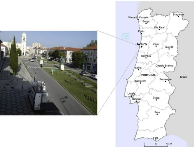
The two-week experimental campaign was conducted in an urban traffic location in Aveiro city centre (Fig. 1). A total of 15 teams originating from various research centres, universities and companies from 12 different countries participated in the campaign.
The city of Aveiro is located in the central region of Portugal (40380N, 8390W), with around 80 000 inhabitants and a total area of approximately 8 km2(INE, 2012) (seeFig. 1). Aveiro is a coastal city, situated on the shores of a coastal lagoon.
Aveiro has a Mediterranean climate, with an annual average temperature of around 15 C, and daily temperature amplitude between 5C and 10C for every month of the year. The annual averages of relative humidity vary from 79% to 88% (IPMA, 2015).
Road traffic is the most significant source of emissions to the atmosphere in the monitoring location, despite the presence of an industrial area located at 10 km from the city centre. The atmo-spheric pollutant concentration, measured in the centre of Aveiro by a traffic station from the national air quality network for 2014, points to annual average values of 31.3
m
g m3 for PM10, 25.1m
g m3for NO2and 211.9m
g m3for CO (QualAr, 2015).2.2. Technical specifications of the reference equipment
During the intercomparison campaign, the IDAD mobile labo-ratory was equipped with standard and reference analysers for
continuous measurement of atmospheric pollutant concentrations and specific sensors for the measurement of meteorological pa-rameters.Table 1shows the measured air pollutants, measurement equipment and their respective methods and measurement range. In addition to the air pollutants, the LabQAr is equipped with a meteorological tower (Vaisala WTX520) containing sensors to conduct continuous measurements of temperature, relative hu-midity, wind speed and direction, atmospheric pressure, precipi-tation and global radiation, at approximately 5 m above ground. The values are acquired instantly in a datalogger that stores the 15-min average per parameter.
2.3. Technical specifications of the sensor nodes
A total of 15 participating teams installed 130 microsensors on LabQAr to monitor various parameters (atmospheric pollutants and meteorological variables) using different measuring principles. Some of the sensors failed during the exercise and the results of others will be used for additional research (examples in sections 2.3.7e2.3.10), thus 27 of the sensors deployed were included in this study.
The different sensor-systems that were installed side-by-side with the reference analysers are based on optical particle coun-ters (OPC), metal oxide semiconductor sensors (MOS), electro-chemical sensors (EC), nondispersive infrared sensors (NDIR) and photoionisation detection sensors (PID). For PM measurements the sensor-systems measure particle counts based on the principle of light scattering.
Table 2presents the measured parameters, technologies and
Fig. 1.Location of the 1st EuNetAir Intercomparison exercise in the city centre of Aveiro. The picture on the left shows the roadside location at which the campaign was carried out.
Table 1
Measured air pollutants, equipment, measurement methods and measurement range of the reference equipment.
Pollutant Equipment Measurement method Measurement range Sulphur dioxide (SO2) Airpointer - Recordum Ultravioletfluorescence (EN 14212) 0e1000mg m3(0e376 ppb)
Nitrogen dioxide/nitrogen oxides (NOx) Environnement AC31M Chemiluminescence (EN 14211) NO: 0e1200mg m3(0e962 ppb)
NO2: 0e500mg m3(0e261 ppb)
Airpointer - Recordum
Carbon monoxide (CO) Environnement CO11M Infrared photometry (EN 14626) 0e100 mg m3(0e86 ppm)
Airpointer - Recordum
Ozone (O3) Environnement O341M Ultraviolet photometry (EN14625) 0e500mg m3(0e250 ppb)
Airpointer - Recordum
PM10 Environnement MP101M Beta-ray absorption method (ISO 10473 equivalent method) 0e200mg m3
PM2.5 Verewa F701
Table 2
Measured parameters, technologies and ranges of the microsensors used in the experimental campaign.
Team Parameter No. Model Type Measurement range
Cambridge CAM10 and 11 boxes NO2 2 Alphasense B4 Electrochemical 0e20 ppm
NO 2 Alphasense B4 Electrochemical 0e20 ppm PM10 2 University of Hertfordshire, CAIR OPC 0.38e17.4mm O3 2 Alphasense B4 Electrochemical 0e5 ppm
CO2 2 SenseAir K30 NDIR 0e5000 ppm
Total VOC 2 Alphasense BH PID 0e5 ppm SO2 2 Alphasense B4 Electrochemical 0e100 ppm
CO 2 Alphasense B4 Electrochemical 0e500 Wind speed 2 Gill WindSonic 2D-Sonic 0e60 ms1
Wind direction 2 Gill WindSonic 2D-Sonic 0e359 Temperature 2 Pt1000 Resistance 30 to 200C
Relative Humidity 2 Honeywell 4000 Thermistor 0e100% RH AUTh-ISAG Temperature 1 MCP9700/9700A Linear Active Thermistor Solid State 40C to 125C
Atmospheric Pressure 1 Motorola MPX4115A Solid State 15e115 kPa Relative Humidity 1 808H5V5 capacitor polymer sensor Solid State 0e100%RH NO2 1 MiCS-2710 Metal oxide 0.05e5 ppm
O3 1 MiCS-2610 Metal oxide 10e1000 ppb
ECN PM10, PM2.5 2 Shinyei ppd42 Optical 0e200mg m3
NO2 2 Citytech3E50 Electrochemical 0e1000 ppb
NanoEnvi NO2 1 Alphasense B4 Electrochemical 0e20 ppm
CO 1 Alphasense B4 Electrochemical 0e1000 ppm O3 1 MiCS-OZ-47 Metal oxide 20e200 ppb
Temperature 1 Sensirion SHT7x Solid State 40 to 123C Relative Humidity 1 Sensirion SHT7x Solid State 0e100% AQMesh NO 3 Alphasense B4 Electrochemical 0e4000 ppb
NO2 3 Alphasense B4 Electrochemical 0e4000 ppb
O3 3 Alphasense B4 Electrochemical 0e1800 ppb
CO 3 Alphasense B4 Electrochemical 0e6000 ppb Temperature 3 Sensirion SHT21 Solid State 20 to 100C Atmospheric Pressure 3 Freescale MPL115A1 Solid State 500e1500 mb Relative Humidity 3 Sensirion SHT21 Solid State 0e100%RH ENEA/Air-Sensor Box CO 1 Alphasense B4 Electrochemical 0e1000 ppm
NO2 1 Alphasense B4 Electrochemical 0e20 ppm
O3 1 Alphasense B4 Electrochemical 0e2 ppm
SO2 1 Alphasense B4 Electrochemical 0e50 ppm
PM10 1 Shinyei PPD20V Optical 0e100mg m3
T 1 Microship TC1047A Solid State 20 to 120C
RH 1 Honeywell HIH5031 Solid State 0e100% VITO/EveryAware SB CO 3 Alphasense CO-BF Electrochemical 0e5000 ppm
CO 3 MiCS-5521 Metal oxide 1e1000 ppm NO2 3 MiCS-2710 Metal oxide 0,05e1 ppm
CO 3 MiCS-5525 Metal oxide 1e1000 ppm Gasoline exh. (CO, H2, HC) 3 Figaro 2201 Metal oxide 10e1000 ppm
Diesel exh. (NO2) 3 Figaro 2201 Metal oxide 0,1e10 ppm
O3 3 MiCS-2610 Metal oxide 10e1000 ppb
VOC 3 AS-MLV Metal oxide NA
T 3 Sensirion SHT21 Solid State 20 to 120C
RH 3 Sensirion SHT21 Solid State 0e100% VITO/Separate sensors CO 1 Alphasense B4 Electrochemical 0e1000 ppm
NO 1 Alphasense B4 Electrochemical 0e20 ppm NO2 1 Alphasense B4 Electrochemical 0e20 ppm
NO2 1 SensorIC NO2 3E 50 Electrochemical 0e50 ppm
NO2 3 AppliedSensor NO2 Metal oxide 0,1e2 ppm
VOC 3 AppliedSensor VOC Metal oxide NA VOC 3 AppliedSensor IAQ Metal oxide NA VOC 3 AppliedSensor IAQ with pulsed heating Metal oxide NA UCL/CCMOSS RH 1 UCL/CCMOSS ImpedimetricMOS 0e100%
measurement ranges of the microsensors used in the experimental campaign.
2.3.1. Cambridge university SNAQ boxes for AQ monitoring
The SNAQ (Sensor Networks for Air Quality) box (henceforth referred to as CAM) is a multi-species instrument package that measures gas phase, particulate and meteorological variables (Table 2). The design is scalable to allow deployment in sensor networks at relatively low cost, and can be operated via mains or battery. They have been successfully deployed for air quality studies in Cambridge (Mead et al., 2013) and London Heathrow Airport (Popoola et al., 2013).
For the purposes of the EuNetAir intercomparison in Aveiro, two boxes were installed on the roof of the IDAD LabQAR. SNAQ10 was mounted approximately 2.5 m above the ground, to a railing on the right-hand side of the vehicle. The Gill sonic on this box was open to all sides. SNAQ11 was installed on the telescopic pole to the left-hand side of the van, at a height of approximately 3.5 m. In this case, the Gill sonic was partially blocked in the westerly direction, due to the mounting pole.
Only the electrochemical (ECC) data from CAM 11 box was used for intercomparison with the IDAD reference instruments and other team's sensors for AQ criteria pollutants. The CAM 10 ECC's showed a very poor response after a power surge around midnight on the 20th October, although the data for CO2, total VOC, OPC and
meteorological variables was unaffected.
Prior to aggregating 20 s data to hourly averages for comparison with the IDAD reference instruments, the following operations were performed on the data: temperature, RH and cross-interference corrections following procedures described inMead et al. (2013); particulate mass loading was derived from the OPC data using the technique discussed and further refined in Di Antonio (2016).
2.3.2. Aristotle university - ISAG-microsensor box
The AUTh-ISAG AQ Microsensor Box (weighting approx. 0.5 kg) was constructed on the basis of the Waspmote™wireless sensor network mote developed by Libellium (http://www.libellium.com) and making use of commercially available sensors. The box design aimed for low power consumption (150 mA when measuring), easy inspection, maintenance, and reduction of thermal noise. Contin-uous airflow is obtained with a microfan installation (consuming 170 mA), while the Box is able to operate via mains or battery. Data were collected on an SD card everyfive minutes and were corrected on the basis of the empirical calibration curves provided by the sensor manufacturers. Data were then averaged over hourly values. The AUTh-ISAG AQ Microsensor Box has been tested in thefield for thefirst time in Aveiro.
2.3.3. ECN - airbox
The AirBox (Hamm et al., 2016) is a weatherproof unit designed to measure a variety of air pollutants in a modular way. The AirBox has been applied since 2013 in the city of Eindhoven in 35 locations to measure PM1, PM2.5, PM10, NO2, O3, UFP, Temp, RH and GPS
coordinates. For PM a modified optical sensor is used (Shinyei PPD42), for NO2a modified electrochemical sensor (Citytech 3E50),
for O3a modified MOS system (based on MiCS 2614) and for UFP the
AeraSense NanoTracer monitor. The PM-sensor is interfaced in such a way that the reflection of individual particles are detected and converted into a mass fraction (see Supplementary Material, Fig. S1). The NO2 sensor is contained in a flow chamber
pro-ceeded by a patented RH and interfering gas conditioning device. The AirBox can be operated via battery or mains. The data is saved temporarily on SD card and is wirelessly communicated by GPRS every 10 min to a network server for on-line validation
purposes and processing. New firmware can be uploaded if requested. A user interface offers data feed, graphical display and metadata. The AirBox can be easily operated on street lighting and requires yearly maintenance.
In the frame of the Aveiro intercomparison exercise the PM and NO2 sensors were evaluated. Due to communication issues, the
equipment did not operate optimally. The modem was not able to contact the mobile network forcing the system to reboot on an hourly basis. Measured data were stored on the SD-card, but due to the rebooting 20 min of data per hour was rejected.
2.3.4. NILUþEnvira -NanoEnvi platform
In collaboration with Envira Ingenieros Asesores, NILU tested the NanoEnvi platform manufactured by Envira. The NanoEnvi platform is a multi-species instrument that measures gas phase variables. In its standard configuration it measures three gases plus ozone, temperature and relative humidity. Depending on the selected configuration it can measure CO, CO2, NO, NO2, O3, H2S,
NH3, COV and SO2. In the configuration for this exercise, NO2, CO
and O3were measured. Data was collected with a temporal
fre-quency offive minutes, and averaged to hourly values if required for the data analysis. The data was not post-processed to correct for temperature and humidity effects or cross-interference with other gases. For the analysis, only the negative concentration values were removed. Negative values were only registered for the NO2sensors
and represented about 20% of the total data. 2.3.5. IDAEA-CSIC - AQMesh node
In collaboration with AQMesh, IDAEA tested the AQMesh pod (22 cm16 cm x 20 cm,<2 Kg) that measured NO, NO2, O3and CO
using Alphasense electrochemical sensors. Pod temperature, RH and atmospheric pressure are also measured using solid-state sensors. A lithium thionyl chloride battery and GPRS communica-tion, with online data access, were used. For the purposes of the EuNetAir intercomparison in Aveiro, four AQMesh pods were installed on the roof of the IDAD Mobile Air Quality Laboratory. Only the data from one of the pods deployed was used given that the other three were affected by RH issues and failed during the exercise. The technical specifications of these sensor nodes (Alphasense, 2013) describe the mechanisms whereby the AQMesh nodes are affected by ambient relative humidity, due to the increasing volume of the internal aqueous acid electrolyte. 2.3.6. ENEA/air-sensor box
In ENEA, at Brindisi Research Centre, a handheld gas sensor system called AirBox based on solid-state gas sensors was designed and implemented. For the purposes of the EuNetAir intercompar-ison in Aveiro, this sensor box (ENEA-AirBox) including CO, NO2, O3,
SO2, PM10, T, RH, was installed on the roof of the IDAD Mobile Air
Quality Laboratory. AirBox uses promising electrochemical gas sensors by Alphasense (CO-B4, NO2-B4, O3-B4, SO2-B4), an Optical
Particle Counter (seeSupplementary Material, Fig. S2) by Shinyei (PPD20V), a relative humidity sensor by Honeywell (HIH5031), and a temperature sensor by Microchip (TC1047A). The AirBox can be operated via battery or mains. The data are saved temporarily on SD card and are wirelessly communicated by GPRS at a programmed sampling rate (in this case, every 15 min) to a network server for validation purposes and post-processing. Over 12 AirBox units have been successfully deployed for air quality studies in Bari (Italy). 2.3.7. VITO - EveryAware SensorBox
The EveryAware SensorBox is a low-cost, portable device to measure the personal exposure to traffic pollution. This device has been developed in the context of the EveryAware FP7 project. Both hardware design and software of the EveryAware SensorBox are
made open source and can be downloaded for free from the project website. This device contains six low-cost gas sensors that react in the presence of traffic pollutants, and O3, VOC, T, and RH sensors for
signal correction purposes. The signals of the 10 sensors are com-bined with machine learning techniques to obtain a more reliable result. The EveryAware SensorBox is equipped with a built-in GPS that determines every second the measurement location, and with a Bluetooth radio allowing transmission of the measurements in real-time to a smartphone. Three EveryAware SensorBoxes have participated in the sensor intercomparison.
Additionally, three NO2, VOC, IAQ, and IAQ with pulsed heating
metal oxide gas sensors from AppliedSensor have been added. Also a number of promising electrochemical gas sensors were installed from AlphaSense (CO-B4, NO-B4, NO2-B4) and SensorIC (NO23D 50).
With additional research the data will be used to evaluate if meteorological conditions and cross sensitivity issues can be overcome by combining the signals of different low-cost gas sensors.
2.3.8. UCL/CCMOSS MOS micro-hotplate for relative humidity sensing
The sensor is based on coated electrodes embedded in a micro-hotplate and a Freescale™KL25Z data logger with its own tem-perature sensor. It exploits an atomic layer deposited 25 nm-thick Al2O3coating, in contrast to conventional polymer-based humidity
sensors (Sensirion, Honeywell, etc.). The relative humidity varia-tions are transduced into capacitance then converted to oscillating voltage period variations with a 200
m
W low power consumption (seeSupplementary Material, Fig. S3). For high (low) relative hu-midity levels, the IDE capacitance increases (decreases), making the oscillating voltage period increase (decrease). The lack of ventila-tion in the package considerably influenced the local atmospheric conditions making the comparison with the relative humidity reference non-direct. However, subsequent measurements per-formed in a climatic chamber gave a±2% relative humidity level accuracy with 2% non-linearity error (Andre et al., 2016).2.3.9. 3S - OdorCheckerOutdoor
Devised to monitor odour-related VOC compositions in thefield, the 3S OdorCheckerOutdoor is an outdoor measurement platform based on experience gained from theMNT-ERA.NETproject VOC-IDS. Temperature cyclic operation of MOX sensors is employed as a key technology which has proved to be both highly sensitive as well as sufficiently selective for low concentrations of pollutants in a high concentration background matrix (Leidinger et al., 2014).
The outdoor device with rugged housing and off-grid power option features two independently controlled MOX sensors and a combined humidity and temperature sensor for reference pur-poses. Outdoor air is actively pumped past the sensors via a closed pneumatic path. Internal measurements and an optional wind sensor are logged to an SD card that also contains an adaptable parameter set for the temperature cycles. The system can be further expanded with sensor modules or a telemetry interface via a general-purpose communication connection.
While the sensor system proved to be quite reliable in a pro-longed field test with distributed installation sites (Reimringer et al., 2015), the device used at Aveiro was affected by shipping damage to the thin-film sensor used for selective measurement. Therefore, no meaningful results could be achieved from the intercomparison experiment.
2.3.10. Siemens AGeGa2O3 based microhotplate sensor
The prototype micro-hotplate sensor installed by Siemens AG is a resistive metal-oxide based gas sensor using Gallium-oxide as the
sensitive layer. It responds non-selectively to a broad range of VOCs and gives an overall indication on VOC concentration in the envi-ronment. The sensor operation temperature is around 800C which is reached using an integrated heater. The novel approach is to manufacture the sensor using a CMOS-compatible process directly on Silicium. Due to its miniaturized size the sensor can be used in pulsed heating mode with a duty cycle of 300 m ONe5s OFF. This greatly reduces the overall power consumption of the sensor sys-tem. Siemens AG has developed the sensors within the project “Environmental Sensors for Energy Efficiency”(ESEE, ENIAC-ED-52, Call 2012-1).
As comparison to state of the art MEMS gas sensors, two different sensing technologies have been operated in parallel to the Ga2O3 based micro-hotplate sensor prototype: two Applied MLV metal oxide sensors using the MOXstick readout platform supplied by JLM Innovation GmbH, and a GAS8616B microsensor from Micronas, measuring temperature and relative humidity as well as employing Platinum (for H2) and Phthalocyanine (for NO2) as gas
sensitive layers for work function based readout.
2.4. Experimental setup
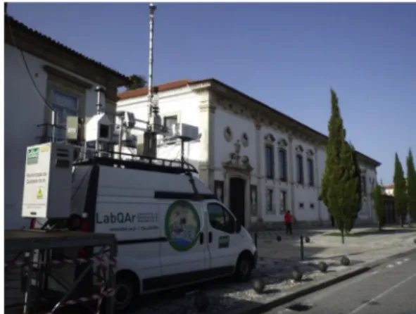
During the intercomparison exercise, the AQ Mobile Laboratory containing reference equipment, micro-sensors and specific sen-sors for the measurement of meteorological parameters was placed on Avenue Santa Joana, near the Cathedral of Aveiro (Fig. 2). The sensors were mainly installed between 2.5 and 3 m above ground on the roof of the mobile laboratory.
The microsensor installations for each team on the top of IDAD LabQAr are presented inSupplementary Material (Fig. S4).
Fig. 2.Set-up of the AQ mobile station and micro-sensors during the 1st EuNetAir
campaign.
Table 3
Results obtained by reference methods. Concentration data are inmg m3(PM10,
PM2.5), ppb (O3, SO2, NO2, NO) and ppm (CO).
Pollutants Average (1 h) Maximum (1 h)
PM10 32 113 PM2.5 15 81 O3 17 44 SO2 1,8 4,2 NO2 16 50 NO 15 139 CO 0,33 1,36
0 25 50 75 100 125 150 175 6: 00 12 :00 18 :00 0:00 6: 00 12 :00 18 :00 0:00 6: 00 12 :00 18 :00 0:00 6: 00 12 :00 18 :00 0:00 6: 00 12 :00 18 :00 0:00 6:00 12 :00 18 :00 0:00 6: 00 12 :00 18 :00 0:00 6: 00 12 :00 18 :00 0:00 6: 00 12 :00 18 :00 0:00 6: 00 12 :00 18 :00 0:00 6: 00 12 :00 18 :00 0:00 6: 00 12 :00 18 :00 0:00 6: 00 12 :00 18 :00 0:00 6: 00 12 :00 18 :00 0:00 6: 00 12 :00 18 :00
13-Oct 14-Oct 15-Oct 16-Oct 17-Oct 18-Oct 19-Oct 20-Oct 21-Oct 22-Oct 23-Oct 24-Oct 25-Oct 26-Oct 27-Oct
PM10 ( μ g.m -3) 0 20 40 60 80 100 120 140 6: 00 12 :00 18 :00 0:00 6: 00 12 :00 18 :00 0:00 6: 00 12 :00 18 :00 0:00 6: 00 12 :00 18 :00 0:00 6: 00 12 :00 18 :00 0:00 6:00 12:00 18:00 0:00 006: 12:00 18:00 0:00 6:00 :0012 18:00 0:00 6:00 12:00 18:00 0:00 6:00 12:00 18:00 000: 6:00 12:00 18:00 0:00 6:00 12:00 18:00 0:00 6:00 12:00 18:00 0:00 6:00 12:00 18:00 0:00 6:00 12:00 18:00 13-Oct 14-Oct 15-Oct 16-Oct 17-Oct 18-Oct 19-Oct 20-Oct 21-Oct 22-Oct 23-Oct 24-Oct 25-Oct 26-Oct 27-Oct
O3 ( μ g.m -3) 0 20 40 60 80 100 120 140 6: 00 12 :00 18 :00 0:00 6:00 12 :00 18 :00 0:00 6:00 12 :00 18 :00 0:00 6:00 12 :00 18 :00 0:00 6:00 12 :00 18 :00 0:00 6:00 12 :00 18 :00 0:00 6:00 12 :00 18 :00 0:00 6:00 12 :00 18 :00 0:00 6:00 12 :00 18 :00 0:00 6:00 12 :00 18 :00 0:00 6:00 12 :00 18 :00 0:00 6:00 12 :00 18 :00 0:00 6:00 12 :00 18 :00 0:00 6:00 12 :00 18 :00 0:00 6:00 12 :00 18 :00 0:00 13-Oct 14-Oct 15-Oct 16-Oct 17-Oct 18-Oct 19-Oct 20-Oct 21-Oct 22-Oct 23-Oct 24-Oct 25-Oct 26-Oct 27-Oct
NO 2 ( μ g.m -3) 0 300 600 900 1200 1500 1800 2100 6: 00 12 :00 18 :00 0:00 6: 00 12 :00 18 :00 0:00 6: 00 12 :00 18 :00 0:00 6: 00 12 :00 18 :00 0:00 6: 00 12 :00 18 :00 0:00 6: 00 12 :00 18 :00 0:00 6: 00 12 :00 18 :00 0:00 6:00 12:00 18:00 0:00 6:00 12:00 18:00 000: 6:00 12:00 18:00 0:00 6:00 12:00 18:00 000: 6:00 12:00 18:00 0:00 6:00 12:00 18:00 000: 6:00 12:00 18:00 0:00 6:00 12:00 18:00 13-Oct 14-Oct 15-Oct 16-Oct 17-Oct 18-Oct 19-Oct 20-Oct 21-Oct 22-Oct 23-Oct 24-Oct 25-Oct 26-Oct 27-Oct
CO (
μ
g.m
-3)
2.5. Data analysis and quality control 2.5.1. Reference methods
After the air quality monitoring campaign, data validation and aggregation was carried out according to the criteria set out in AQD 2008/50/EC.
The timestamp of the measurements is calculated at the upper limit of the integration interval. For example, the average time referenced to 01:00 p.m. is the average concentration observed between 12:00 a.m. and 01:00 p.m.
During the experiment the O3 analyser was checked using a
portable ozone generator SONIMIX 3022-2000. The NOx, SO2and
CO analysers were also checked using certified gas cylinders.
2.5.2. Basic microsensor data analysis
Some of the installed AQ microsensors output results are in concentration units while others provide voltage or frequency data. Therefore, pre-processing of raw data was necessary to proceed to the conversion into concentration units. After the reference data was made available, each team was responsible for the conversion process of their data.
Four temporal sampling frequencies were used by groups participating in the exercise: one, five, 15 min, and one-hour. In order to maximize the dataset made available for analysis, sensor data that were not recorded on an hourly basis were averaged to one-hour values as follows:
Hourly Valuej¼Pni¼j1 Parameteri nj ; j¼1;…;24, And nj ¼ the 0 20 40 60 80 100 0 5 10 15 20 25 30 35 6: 00 12 :00 18 :00 0:00 6: 00 12 :00 18 :00 0:00 6: 00 12 :00 18 :00 0:00 6: 00 12 :00 18 :00 0:00 6: 00 12 :00 18 :00 0:00 6: 00 12 :00 18 :00 0:00 6: 00 12 :00 18 :00 0:00 6: 00 12 :00 18 :00 0:00 6: 00 12 :00 18 :00 0:00 6: 00 12 :00 18 :00 0:00 6: 00 12 :00 18 :00 0:00 6: 00 12 :00 18 :00 0:00 6:00 12 :00 18 :00 0:00 6: 00 12 :00 18 :00 0:00 6:00 12:00 18:00 13-Oct 14-Oct 15-Oct 16-Oct 17-Oct 18-Oct 19-Oct 20-Oct 21-Oct 22-Oct 23-Oct 24-Oct 25-Oct 26-Oct 27-Oct
Rela
ve Humidity (%)
Temperature
(
oC)
Temperature RelaƟve Humidity
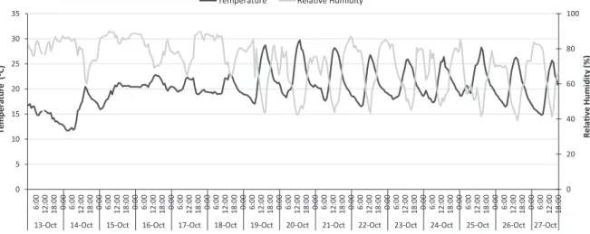
Fig. 4.Temporal distribution of hourly averages of temperature and relative humidity.
Table 4
Statistical indicators comparing the data from the sensor platforms with the reference data. N is the number of values employed in the computation. Concentration data are in
mg m3(PM10, PM2.5), ppb (O
3, SO2, NO2, NO) and ppm (CO).
Pollutants Sensor node Collection efficiency (%) MBE r2 CRMSE N NMSE FB FOEX MAE
PM10 ENEA/AirSensorBox 47 15.3 0.33 25 166 10.27 0.49 15.06 21.15 PM10 CAM_10 93 79.7 0.13 76.9 326 2.41 1.11 43.88 80.91 PM10 CAM_11 93 126.2 0.15 110.9 326 2.15 1.33 49.69 125.10 PM10 ECN_Box_10 82 19.0 0.33 26.3 288 3.56 0.54 29.58 24.57 PM10 ECN_Box_38 90 18.5 0.36 23.8 317 3.51 0.49 31.45 23.61 PM2.5 CAM_10 93 11.1 0.07 19.3 326 3.42 0.56 23.7 17.15 PM2.5 ECN_Box_10 82 2.6 0.23 14 288 4.62 0.27 10.55 11.26 PM2.5 ECN_Box_38 90 3.8 0.27 13.4 317 4.38 0.27 16.03 11.11 O3 ENEA/AirSensorBox 44 19.2 0.13 16.1 155 2.52 0.67 41.61 22.12 O3 NanoEnvi 61 6.5 0.77 7.7 217 3.86 0.33 32.95 7.66 O3 CAM_11 73 15.7 0.14 18.2 257 2.74 0.71 30.23 21.50 O3 AQMesh 37 0.0 0.70 3.3 132 4.25 0.19 7.25 2.40 O3 ISAG 89 356.1 0.12 187.4 314 1.37 1.82 50 360.12 SO2 ENEA/AirSensorBox 44 23.4 0.20 9.2 157 1.26 1.74 48.73 23.47 SO2 CAM_11 93 29.1 0.09 12.4 326 1.27 1.78 50 29.10 NO2 CAM_11 93 2.3 0.84 4.3 326 9.30 0.35 44.15 5.61 NO2 ENEA/AirSensorBox 46 17.7 0.06 15.0 164 2.45 0.69 39.02 20.17 NO2 NanoEnvi 50 13.1 0.57 18.8 174 3.72 0.51 31.03 14.93 NO2 ECN_Box_10 80 1.0 0.89 4.4 266 18.92 0.81 50 4.95 NO2 AQMesh 37 0.0 0.89 1.9 132 5.69 0.58 5.38 1.46 NO2 ISAG 89 349.5 0.02 33.5 312 1.10 1.84 50 16.17 CO ENEA/AirSensorBox 44 0.0 0.76 0,1 154 6.49 0.09 22.08 0.09 CO NanoEnvi 61 0.1 0.53 0,1 217 4.07 0.14 29.72 0.10 CO CAM_11 92 0.2 0.87 0.1 325 14.65 0.72 47.53 0.18 CO AQMesh 99 0.0 0.86 0.1 350 5.03 0.00 0.72 0.05 NO CAM_11 93 9.5 0.34 14.3 328 4.87 0.34 26.62 12.02 NO AQMesh 37 0.0 0.80 1.9 132 6.47 0.99 3.85 1.51
number of samples available for hourj. Thus data from 00:01 up to 01:00 was used for the calculation of the average value for time 01:00, and so on.
The comparison between the available datasets was made with the aid of some basic statistical measures as well as by employing indices that are widely used and accepted for data comparisons, and are presented inSupplementary Material (Table S1): Mean Bias ErroreMBE, Correlation Coefficienter, Centred Root Mean Square ErroreCRMSE, Root Mean Square ErroreRMSE, Normalised Mean
Square ErroreNMSE, Fractional BiaseFB, Factor of Exceedancee FOEX, Mean Absolute ErroreMAE.
2.5.3. Advanced microsensor data analysis
While pre-processing the data, cases with missing values were identified that may prevent further analysis if traditional statistical methods are applied. For this reason, the unsupervised machine learning method of Self Organizing Maps (SOMs) was used, as part of a Computational Intelligence approach for further data analysis
and modelling (Kolehmainen, 2004).
SOMs (one of the best unsupervised neural learning algorithms) are actually a mapping of high-dimensional data inputs onto ele-ments of a low-dimensional array. Their function is tofind proto-type vectors that represent the input data set and at the same time depict a continuous mapping from the input space to a lattice, which is considered to be a mathematical construct topologically representing the“interrelationships”between data from the initial
data set. Thus, SOMs are ideal for compressing information while preserving the topological relationships of the data. SOMs may also be considered as a data analysis and visualization technique that reduces the dimensions of data through the use of self-organizing neural networks, in order to simplify the understanding and interpretation of high dimensional data. The way SOMs proceed in dimension reduction is by the production of a map (of usually two dimensions) which visualizes the“similarities”of data by grouping
similar data items together (Kaltech et al., 2007).
SOMs consist of neurons, each one of which is a set of co-efficients corresponding to the variables of the data set. The SOM Toolbox1 for MATLAB was used to implement the SOMs in the current study. Through the training process, the map of neurons represents (via the weighting vectors) the actual data vectors within the studied dataset. SOMs visualization is commonly sup-ported by the unified distance matrix (U-matrix), which represents the Euclidean distance between neighbouring neurons (data). The U-matrix thus depicts the relations between neighbouring data, where the neuron colour represents the distance from that neuron to its surrounding neighbours. Thus, low values (commonly visualised with the aid of dark blue colours) represent tight clusters of data, and high values (commonly visualised with yellow-red colours) represent a clear separation between neighbouring neurons.
2.5.4. Overall sensor comparison
In addition to the statistical metrics described in 2.5.2, the Target diagram (Jollif et al., 2009) is being used for evaluating sensor data against reference measurements simultaneously. This diagram is an evolution of the Taylor diagram (Taylor, 2001), which was based on the geometrical relation between the CRMSE and the standard deviations of both reference and studied data (here sensor data). The Target diagram allows extending the notion of the Taylor diagram by distinguishing within the RMSE the contributions from (a) the MBE and (b) the CRMSE. In fact, this composite plot repre-sents the normalised RMSE as the quadratic sum of the normalised MBE on the Y-axis versus the normalised CRMSE on the x-axis. The distance between each point and the origin represents the nor-malised RMSE for each platform sensor. Furthermore, target scores are plotted in the left quadrant of the diagram when the standard deviation of the sensor responses is lower than the one of the references measurements and conversely. In the original approach of the Target diagram, RMSE, MBE and CRMSE can be normalised using the standard deviation of the reference measurements
s
0.Finally, sensors with random error equivalent to the variance of the observations stand in the circle area of radius 1. Target scores inside this circle indicate a variance of the residuals between sensor and reference measurement equal or lower than the variance of the reference measurements. In fact, sensors within the target circle are better predictors of the reference measurements than mean
concentrations over the whole sampling period. The target diagram normalised with
s
0has been recently implemented (Spinelle et al., 2015). It established a relaxed quality objective.Thunis et al., 2013 andPernigotti et al., 2013have implemented a modification to this approach, normalizing CRMSE, MBE and RMSE with the measure-ment uncertainty of the sensor and reference values. In this modification, the circle area is used to check a Model Quality Objective corresponding to the Data Quality Objective of the Air Quality directive (2008/50/EC) corresponding to a target level of measurements uncertainty.3. Results and discussion
3.1. Results obtained by reference methods
Results obtained by reference methods during the measurement campaign are summarised inTable 3.
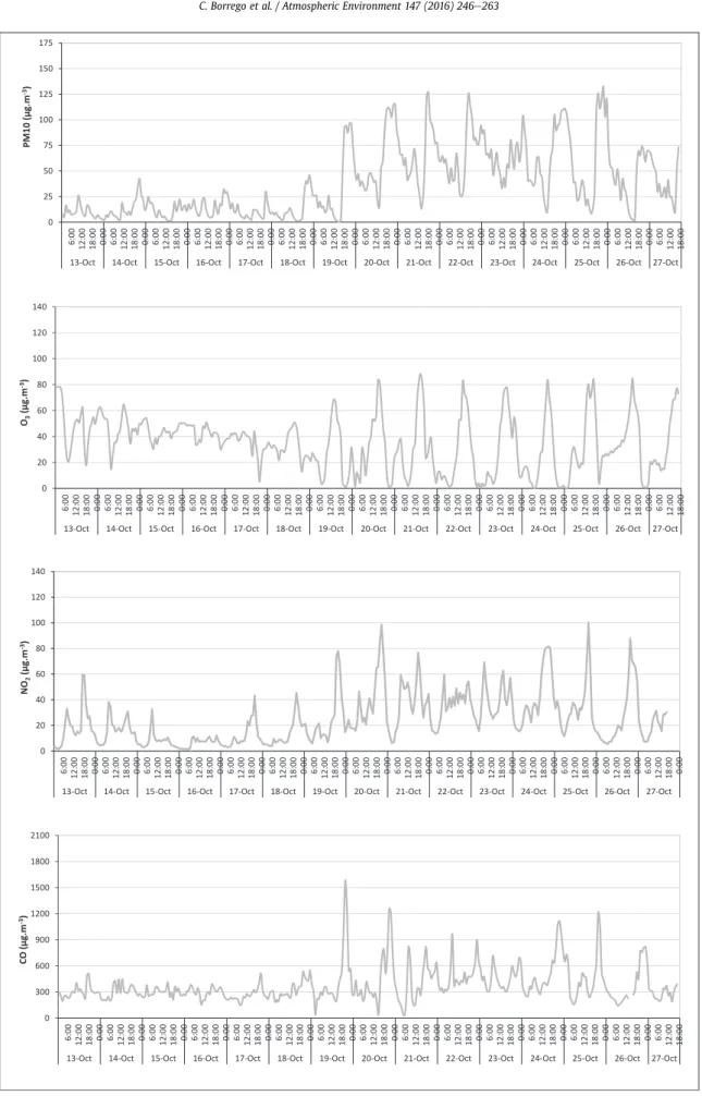
Fig. 3shows the temporal distribution for PM10, O3, NO2and CO
hourly average concentrations. Over the two-week campaign, the PM10 daily limit of 50
m
g m3for the protection of human health was exceeded six times from the 20th to the 25th of October. This was due to the associated traffic emissions and meteorological conditions and also to the simultaneous occurrence of natural events with the transport of particles from North Africa (APA, 2015). Fig. 4presents the obtained values for meteorological parame-ters temperature and relative humidity in the monitoring site for the experimental campaign period. Global radiation, precipitation, wind direction and wind speed profiles are included in Supplementary Material (Figs. S5 and S6).Regarding meteorological conditions, it is noticeable that in the
first week of the experimental campaign, long periods of sustained precipitation were observed (total of 75.4 mm), high relative hu-midity (average: 79%, range: 44e90%), relatively low temperatures between 15C and 20C, and comparatively high wind speeds (average: 2.2 m/s, range: 0.1e5.6 m/s), whereas in the second week the meteorological conditions changed, exhibiting no precipitation, high temperatures (average: 21C, range: 15e30C), lower relative humidity (average: 65%, range: 39e87%) and lower wind velocities (average 0.6 m/s, range: 0.1e1.5 m/s).
3.2. Results obtained by microsensors 3.2.1. Basic statistics and indices
The evaluation of the sensor performance was carried out using the observed data from the sensor platforms and the data from the
Fig. 7.Sensor modules vs. reference instrumentation correlation plots for SO2. All axis units are in ppb.
reference instrumentation to compute descriptive statistics re-ported inSupplementary Material (Table S1). Results are presented inTable 4and discussed in this section.
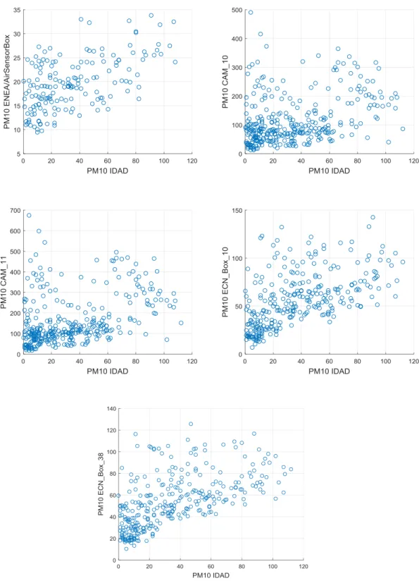
3.2.1.1. PM - particulate matter. For PM10, the results show a poor correlation between the reference and the available measurements, with r2¼0.36 being the maximum value achieved for ECN_Box_38. The lowest absolute value of the CRMSE is found for ECN_Box_38, ENEA/AirSensorBox and ECN_Box_10, while for the MBE the situ-ation is different only for ENEA/AirSensorBox, now being the best.
The CAM sensors demonstrate low correlation and higher MBE and MAE, and a strong tendency for overestimation (FOEX close toþ50), although they also demonstrate lower NMSE. Thefindings are supported byFig. 5, which presents the correlation plots for the aforementioned measurements. The overall poor performance is visible via the scattering of the values and their deviation from the correlation line.
For PM2.5, results are available for only three platforms and are poor in terms of representing the reference measurements: the best performance comes from ECN_Box_38 with r2¼0.27 and a
value of the CRMSE equal to 13.4. The CAM sensor response reveals a low correlation and a higher NMSE (¼10.27) and absolute FB (0.56), as well as higher MBE and MAE. In literature, examples of PM field tests with optical sensors reported higher r2 values ranging from 0,86 to 0,89 (Gao et al., 2015) or 0.55e0.60 (Holstius et al., 2014).
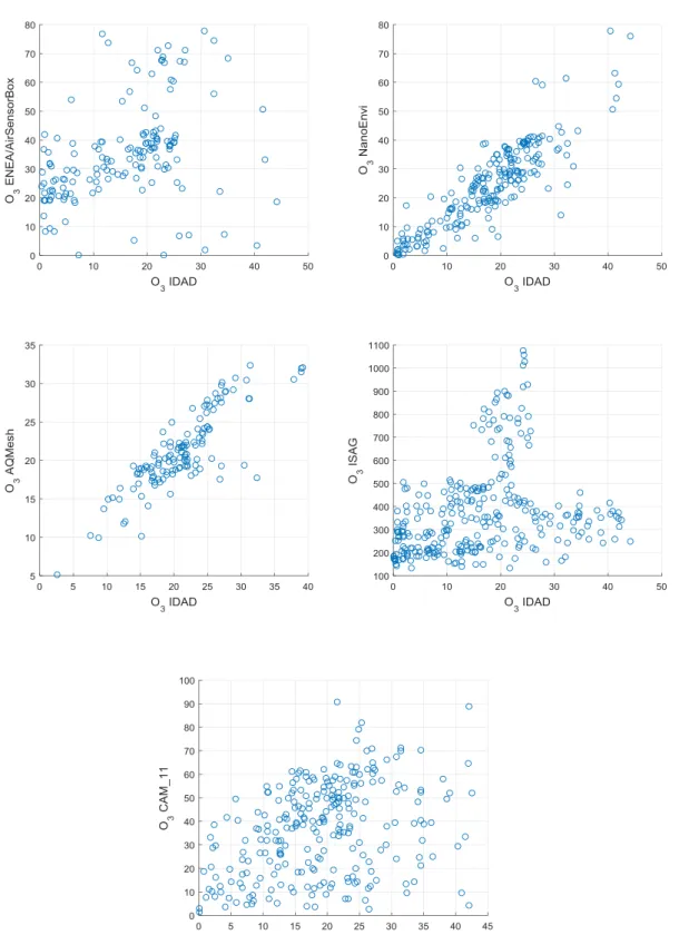
3.2.1.2. O3 e ozone. For O3 the best results come from IDAEA/
AQMesh and NanoEnvi platforms, both of them having the lowest CRMSE and MBE, and the higher r2(above 0.7). All sensors have quite low NMSE, but IDAEA/AQMesh exhibits the lowest MBE and
MAE (followed by NanoEnvi). ENEA/AirSensorBox, ISAG and CAM_11 platforms demonstrate poor correlations coefficients, with r2values below 0.2, while they also present higher CRMSE and MBE, with ISAG being by far the worst (MBE~350).
The fact that ISAG has the overall lowest NMSE but also the lowest r2underlines not only the poor performance of the specific sensor but also the limitations of the classic error-oriented metric in weighting sensor performance. By taking into account FB and FOEX, IDAEA/AQMesh and NanoEnvi have indeed the best perfor-mance, followed by CAM and ENEA/AirSensorBox that have an equivalent performance. These findings are supported by the
Fig. 9.Sensor modules vs. reference instrumentation correlation plots for CO. All axis units are in ppm.
correlation plots (Fig. 6) where IDAEA/AQMesh and NanoEnvi show a clear overall agreement with IDAD, CAM_11 and ENEA/Air-SensorBox demonstrate value scattering, while ISAG demonstrates almost no correlation at all.
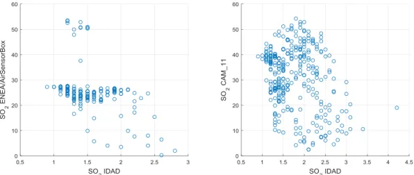
3.2.1.3. SO2- sulphur dioxide. There are only two measurement sets available for SO2, coming from ENEA/AirSensorBox and CAM_11,
both demonstrating poor performance with low correlation
coef-ficient and metrics values (Fig. 7). The best performance comes from ENEA/AirSensorBox with r2¼0.20 and a value of the MAE equal to 23.47. For the CAM_11 sensor responses reveal a low cor-relation coefficient, with r2¼0.09 and a value of the MAE equal to 29.10.
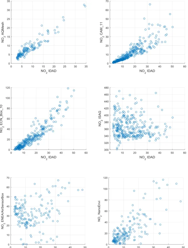
3.2.1.4. NO2- nitrogen dioxide. For NO2, six sensor platforms were
compared; the higher correlations and lowest bias are obtained for IDAEA/AQMesh, ECN_Box_10 and CAM_11 with r2>0.8 andМВЕ
close to zero. The NanoEnvi platform demonstrates a good corre-lation of 0.6, but the ENEA/AirSensorBox and ISAG platforms exhibit a poor correlation of below 0.1. ENEA/AirSensorBox and NanoEnvi demonstrate the higher FOEX values (above 30). IDAEA/AQMesh has the best FOEX index (5.38, suggesting the best balance in terms of over/underestimation), and the best MBE. ISAG demonstrates the worst performance overall.
Thesefindings are supported byFig. 8, which presents the cor-relation plots among reference values for NO2and sensor modules.
A significant correlation is evident for IDAEA/AQMesh, CAM_11 and ECN sensor boxes. Possible non-linearities are suggested in the plot for CAM_11. In the same plot higher absolute errors are found at higher values of reference concentration.
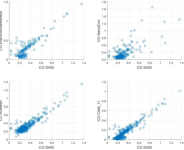
3.2.1.5. CO - carbon monoxide. For CO, four platforms were compared. All the platforms present a satisfactory correlation (r2>0.5). The CAM_11 and IDAEA/AQMesh have the highest cor-relations (r2>0.8).
Fig. 9demonstrates how all the sensor boxes except NanoEnvi exhibit significant correlation and linearity among all the relevant range of values. Highest relative errors can be expected at the low end of the concentration range.
3.2.1.6. NO - nitrogen monoxide. For NO, two platforms were available, IDAEA/AQMesh and CAM_11. Good correlation (r2¼0.8) and small bias is observed for the IDAEA/AQMesh sensor while the results show a weak correlation with r2¼0.3 for CAM_11.
Fig. 10shows correlation plots for IDAEA/AQMesh and CAM_11 sensor boxes. Both express a good correlation with better values obtained by CAM_11. The CAM_11 plot reveals two different areas of relationships, thus suggesting the possibility of drift or strong interference.
3.2.2. Insights on sensor behaviour and performance: SOM results The SOM graph can be used to study the overall behaviour and
profile characteristics of the sensors. It allows investigation of the patterns of sensor data, and to compare them with the patterns of the reference dataset as well as with those of other sensors. The following section focuses on those pollutant datasets that have provided the best statistical metric results in the sensor evaluation presented in chapter 3.2.1, which are O3, NO2and CO. On the basis
of the information provided in chapter 2.5.3 about the SOM method, the “interrelationships” between sensor data are pre-sented as areas of similar colour and shape in the SOM graphs, identified with the aid of the U-matrix graph.
3.2.2.1. SOM of ozone data. The IDAD measurements as well as the U-matrix indicate that there are three main areas of the specific sensor profile, each one related to a different part of the O3
behaviour (marked with red ellipses in the IDAD SOM): the upper area corresponds to low ozone conditions and coincides with me-dium to low temperatures, thus it can be attributed to low ozone productivity dynamics in the Aveiro area, and is roughly repro-duced by each microsensor node (Fig. 11). The lower right area denotes high ozone values and appears in parallel with the highest temperature values, thus suggesting the typical ozone production mechanism with the presence of solar radiation. This area is mostly
represented by NanoEnvi measurements. There is also a third area (lower left on IDAD SOM), that suggests medium to high ozone concentrations, but it appears in parallel with low temperature values, relatively high RH and low NO values (indicating possible ozone transportation in the Aveiro area during the night, and mostly represented in IDAEA/ AQMesh and CAM_11 measure-ments). This suggests that contrasting sensor nodes may have, in addition to varying performance statistics, differences in their behaviour and in their ability to“map”real world phenomena, a
finding that deserves additional research.
3.2.2.2. SOM of NO2data. The IDAD measurements as well as the U-matrix indicate that there are two main areas of the specific sensor profile, each one related to a different part of the NO2
behaviour (marked with red squares in the IDAD SOM): the upper area corresponds to high NO2concentrations and coincides with a
wide range of temperatures yet mostly with medium and high values, thus suggesting a production (in part) by the oxidization of NO in the presence of O3(Fig. 12). Among all sensors with available
data, ECN and IDAEA/AQMesh are closest to the pattern of the IDAD measurements, followed by CAM_11 and NanoEnvi. ENEA/Air-SensorBox follows the basic patterns but demonstrates strange
behaviour in low temperatures, while ISAG is clearly not related to IDAD and to any other sensor data.
3.2.2.3. SOM for CO data. There are two main areas of the specific sensor profile, each one related to a different part of the CO behaviour (marked with red squares in the IDAD SOM): the upper area corresponds to low CO concentrations and coincides with medium temperature ranges (Fig. 13). The highest temperature area does seem to coincide with the absence of high CO values, indi-cating combustion activities during the colder part of the mea-surement campaign as a possible main source. Among sensors with available data, IDAEA/AQMesh and CAM_11 seem to better match the profile of the reference measurements, closely followed by ENEA/AirSensorBox, while NanoEnvi also demonstrates a good response in terms of profile similarities with reference data. 3.2.3. Overall sensor intercomparison: the target diagram
The target diagram for all sensor platforms is presented in Fig. 14. A few platforms fall within the target circle showing a RMSE within the standard deviation of reference measurements for: the O3, NO2, NO and CO IDAEA/AQMesh sensors, the CAM_10 and
CAM_11 NO2 sensors, the ENEA/AirSensorBox and NanoEnvi CO
sensor and the PM2.5 ECN sensors. Another set of sensors, the CO CAM_11, the PM10 ECN and ENEA/AirSensorBox Sensors and the O3
NanoEnvi sensor lay on the edge of the target circle. Conversely, the NO2and O3ISAG sensors and the SO2sensor of ENEA/AirSensorBox
and CAM_11 fall out of the range of the target values with nor-malised RMSE of up to 60 (see Table 4) demonstrating lack of agreement with reference measurements.
No strong pattern can be observed regarding the preponderance of bias or random noise out of the target diagram. In fact, similar ranges of target scores are observed for the normalised bias and CRMSE on both x and y-axis. A set of sensors falls on thefirst di-agonal of the diagram showing equal scores for MBE and CRMSE. Approximately the same number of target scores fall on the right and left quadrants of the diagram, indicating that none of the sensor or reference measurements have a systematic wider range of values. Noticeably, the IDAEA/AQMesh target scores shows the same pattern for O3, NO2, NO and CO sensors: absence of MBE,
lower standard deviations for the sensors values compared to the reference measurements and good correlation with references values. For the rest of the platforms, the sensor scores are more
scattered. 4. Conclusions
Developments in AQ microsensor technologies allow for their comparison with reference instrumentation in order to evaluate their ability to support and complement standard monitoring procedures. This also permits assessment of microsensors for their use in obtaining data with high spatial and temporal resolution and thus to support air quality related, quality of life information ser-vices. In the frame of thefirstfield-based intercomparison exercise in Aveiro, Portugal, both aspects were investigated.
The overall performance of the sensors in terms of their statis-tical metrics and measurement profile suggest that the relevant microsensor platforms, if supported by the proper post processing and data modelling tools, can be used for providing spatially and temporally useful information for air quality levels.
In terms of pollutants, O3, CO, and NO2were the three gases that
were measured in a relatively successful way from the tested platforms, and the gases that were profiled in a satisfactory way. In this case correlations up to approximately 0.9 were achieved for some sensors. For PM and SO2, the results show a poor performance
with low correlation coefficients between the reference and the available measurements.
It should be noted that the results are only representative of the measurements conditions during the campaign. Results may vary under different weather conditions or for longer periods. In some cases, the performance of microsensors is temperature-dependent and thus may decrease significantly during warmer months. In the present exercise long-term drifts were not evaluated, because the campaign was performed during two weeks.
The real-time collected data from microsensors combined with standard monitoring techniques have an enormous potential to be applied in new strategies for air quality control, rapid mapping of air pollution at high spatial detail, validation of atmospheric dispersion models or evaluation of population exposure, and for the development of user-tailored, georeferenced, human centred,
quality of life information services. The studied microsensors exhibit particular potential with regard to urban-scale mapping of air quality, where their current inaccuracies can be offset to some extent by the simultaneous use of reference equipment, but where the lower cost of microsensors allows for measurements of air quality at a significantly higher spatial density than was previously possible with reference equipment alone.
The evaluation of the 1st EuNetAir campaign results shows that microsensors can be a promising technique for air quality moni-toring, and confirm the relevance of establishing an evaluation protocol approaching issues as sensitivity, selectivity, short and long term stability, model equation and data validation, as well as calibration.
This joint experimental campaign must be seen as afirst step to the research and development of microsensors for pollutants monitoring, contributing to the evaluation of sensor performance infield exercises. As part of the present Air Quality Joint Exercise, additional analysis is being prepared for a second publication, including the comparison of technical requirements of the sensor nodes, measurement uncertainty and calibration of microsensors. Acknowledgements
The authors would like to acknowledge the support of COST Action TD 1105eEuropean Network on New Sensing Technologies for Air-Pollution Control and Environmental Sustainability e EuNetAir.
The authors would like to acknowledge the support of the Municipality of Aveiro.
The authors wish to acknowledge the support of M. Gerboles of the Institute for Environment and Sustainability of the Joint Research Centre of the European Commission on the evaluation of the sensors.
The UCL authors acknowledge the FP7 EU SOIHITS project for funding (grant agreement no 288481) and especially the partners UCAM (F. Udrea), CCMOSS (S. Z. Ali, F. Chowdhury) and UCL (D. Flandre).
The IDAEA-CSIC authors would like to acknowledge AQMesh for kindly providing the AQMesh pods. Support is acknowledged to Generalitat de Catalunya 2014 SGR33.
The NILU authors would like to acknowledge ENVIRA Ingenieros Asesores for participating in the campaign with the NanoEnvi platform.
Appendix A. Supplementary data
Supplementary data related to this article can be found athttp:// dx.doi.org/10.1016/j.atmosenv.2016.09.050.
References
Afzal, A., Cioffi, N., Sabbatini, L., Torsi, L., 2012. NOx sensors based on semi-conducting metal oxide nanostructures: progress and perspectives. Sens. Ac-tuators B Chem. 171e172, 25e42.http://dx.doi.org/10.1016/j.snb.2012.05.026. AugusteSeptember 2012, ISSN 0925-4005.
Aleixandre, M., Gerboles, M., 2012. Review of small commercial sensors for indic-ative monitoring of ambient gas. Chem. Eng. Trans. 30, 1e6.http://dx.doi.org/ 10.3303/CET1230029.
Alphasense, 2013. Alphasense Application Note AAN106: Humidity Extremes: Drying Out and Water Absorption - AAN106. Available at: http://www. alphasense.com/WEB1213/wp-content/uploads/2013/07/AAN_106.pdf. APA (Portuguese Environment Agency), 2015. Transporte de partículas e poeiras
naturais com origem em regi~oesaridas dos desertos do Norte deAfrica. http:// www.apambiente.pt/index.php?
ref¼16&subref¼82&sub2ref¼316&sub3ref¼941(Accessed July 2015).
Andre, N., Li, G., Pollissard-Quatremere, G., Couniot, N., Gerard, P., Ali, Z., Udrea, F., Zeng, Y., Francis, L.A., Flandre, D., 2016. SOI sensing platforms for water vapour and light detection. In: CMOSET Conference, Session C5, May 25e27, Montreal, Canada.
Fig. 14.Target diagram for the microsensors and sensor platforms evaluated in this
study. The SO2sensors have not been plotted as they fell outside the limits with higher
Castell, N., Kobernus, M., Liu, H.-Y., Schneider, P., Lahoz, W., Berre, A.J., Noll, J., 2015. Mobile technologies and services for environmental monitoring: the Citi-Sense-MOB approach. Urban Clim. 14 (3), 370e382.
Castell, N., Viana, M., Minguillon, M.C., Guerreiro, C., Querol, X., 2013. Real-world Application of New Sensor Technologies for Air Quality Monitoring. ETC/ACM Technical Paper 2013/16. Copenhagen. Available at:http://acm.eionet.europa. eu/reports/ETCACM_TP_2013_16_new_AQ_SensorTechn.
De Vito, S., Massera, E., Piga, M., Martinotto, L., Di Francia, G., 2008. Onfield cali-bration of an electronic nose for benzene estimation in an urban pollution monitoring scenario. Sens. Actuator B Chem. 192 (2), 750e757.
Di Antonio, A., February 2016. Field Characterisation of Novel Portable PM Sensors Using Long-term Measurements (MSc Thesis). Department of Chemistry, Uni-versity of Cambridge.
EC WG, 2010. Guide to the Demonstration of Equivalence of Ambient Air Moni-toring Methods. Report by EC Working Group on Guidance. Available at:ec. europa.eu/environment/air/quality/legislation/pdf/equivalence.pdf (Accessed 28 October 2015).
EEA (European Environment Agency), 2013. Air Quality in Europee2013 Report. EEA Report. No. 9/2013, Copenhagen, 112 pages.
EEA (European Environment Agency), 2014. Air Quality in Europee2014 Report. EEA Report. No. 5/2014, Copenhagen, 80 pages.
EUD (European Union Directive), 2008. Directive 2008/50/EC of the European Parliament and of the Council of 21 May 2008 on ambient air quality and cleaner air for Europe. Off. J. Eur. Union L152.
Gao, M., Cao, J., Seto, E., 2015. A distributed network of low-cost continuous reading sensors to measure spatiotemporal variations of PM2.5 in Xi'an, China. Environ. Pollut. 199C, 56e65.http://dx.doi.org/10.1016/j.envpol.2015.01.013.
Hamm, N.A.S., Van Lochem, M., Hoek, G., Otjes, R.P., Van der Sterren, S., Verhoeven, H., 2016. The Invisible Made Visible: Science and Technology.link. springer.com/book/10.1007/978-3-319-26940-5.
Heimann, I., Bright, V.B., McLeod, M.W., Mead, M.I., Popoola, O.A.M., Stewart, G.B., Jones, R.L., July 2015. Source attribution of air pollution by spatial scale sepa-ration using high spatial density networks of low cost air quality sensors. Atmos. Environ. 113, 10e19.http://dx.doi.org/10.1016/j.atmosenv.2015.04.057. ISSN 1352-2310.
Holstius, D.M., Pillarisetti, A., Smith, K.R., Seto, E., 2014. Field calibrations of a low-cost aerosol sensor at a regulatory monitoring site in California. Atmos. Meas. Technol. 7, 1121e1131.http://dx.doi.org/10.5194/amt-7-1121-2014.
INE (Instituto Nacional de Estatística I.P.), 2012. Censos 2011 Resultados Definitivos - Regiao Centro, ISBN 978-989-25-0184-0. Lisboa~ .
IPMA (Instituto Portugu^es do Mar e da Atmosfera), 2015. Normais Climatologicas 1981e2010. Available in: https://www.ipma.pt/pt/oclima/normais.clima/
(Accessed in July 2015).
IUTA, BAuA, BG RCI, VCI, IFA, TUD, 2011. Tiered Approach to an Exposure Mea-surement and Assessment of Nanoscale Aerosols Released from Engineered Nanomaterials in Workplace Operations. Germany. Available at:https://www. vci.de/vci/downloads-vci/tiered-approach.pdf.
Jolliff, J.K., Kindle, J.C., Shulman, I., Penta, B., Friedrichs, M.A.M., Helber, R., Arnone, R.A., 2009. Summary diagrams for coupled hydrodynamic-ecosystem model skill assessment. J. Mar. Syst. 76 (February (1e2)), 64e82.
Kaltech, A.M., Hjorth, P., Berndtsson, R., 2007. Review of the self-organizing map (SOM) approach in water resources: analysis, modelling and application. En-viron. Model. Softw. 23 (7), 835e845. http://dx.doi.org/10.1016/ j.envsoft.2007.10.001.
Kolehmainen, M.T., 2004. Data Exploration with Self-organizing Maps in Environ-mental Informatics and Bioinformatics. Helsinki University of Technology. Available at:http://lib.tkk.fi/Diss/2004/isbn951270000X/.
Kumar, P., Morawska, L., Martani, C., Biskos, G., Neophytou, M., Di Sabatino, S., Bell, M., Norford, L., Britter, R., 2015. The rise of microsensing for managing air pollution in cities. Environ. Int. 75, 199e205. http://dx.doi.org/10.1016/ j.envint.2014.11.019.
Leidinger, M., Sauerwald, T., Reimringer, W., Ventura, G., Schuetze, A., 2014. Selec-tive detection of hazardous VOCs for indoor air quality applications using a virtual gas sensor array. J. Sens. Sens. Syst. 3, 253e263. http://dx.doi.org/ 10.5194/jsss-3-253-2014.
Lim, S.S., Vos, T., Flaxman, A.D., Danaei, G., Shibuya, K., Adair-Rohani, H., et al., 2012. A comparative risk assessment of burden of disease and injury attributable to 67 risk factors and risk factor clusters in 21 regions, 1990e2010: a systematic
analysis for the global burden of disease study 2010. Lancet 380 (9859), 2224e2260.http://dx.doi.org/10.1016/S0140-6736(12)61766-8.
Mead, M.I., Popoola, O. a. M., Stewart, G.B., Landshoff, P., Calleja, M., Hayes, M., Baldovi, J.J., McLeod, M.W., Hodgson, T.F., Dicks, J., Lewis, A., Cohen, J., Baron, R., Saffell, J.R., Jones, R.L., 2013. The use of electrochemical sensors for monitoring urban air quality in low-cost, high-density networks. Atmos. Environ. 70, 186e203.http://dx.doi.org/10.1016/j.atmosenv.2012.11.060.
Penza, M., Suriano, D., Villani, M.G., Spinelle, L., Gerboles, M., 2014. Towards air quality indices in smart cities by calibrated low-cost sensors applied to net-works. In: IEEE SENSORS 2014 Proc. 2012e2017. http://dx.doi.org/10.1109/ ICSENS.2014.6985429.
Pernigotti, D., Gerboles, M., Belis, C.A., Thunis, P., 2013. Model quality objectives based on measurement uncertainty. PartII: NO2and PM10. Atmos. Environ. 79,
869e878.http://dx.doi.org/10.1016/j.atmosenv.2013.07.045.
Popoola, O., Mead, I., Bright, V., Baron, R., Saffell, J., Stewart, G., Kaye, P., Jones, R., 2013. A portable low-cost high density sensor network for air quality at london heathrow airport. In: EGU General Assembly 2013, Held 7-12 April, 2013 in Vienna, Austria id. EGU2013e1907. http://wwwdev.snaq.org/posters/EGU_ OAMP_2013.pdf.
QualAr, 2015.http://qualar.apambiente.pt/.
Reimringer, W., Rachel, T., Conrad, C., Schuetze, A., 2015. MOX sensor platform in outdoor odor monitoring. In: Fourth Scientific Meeting EuNetAir. Linkoping University, Linkoping, Sweden.http://dx.doi.org/10.5162/4EuNetAir2015/12. Snyder, E., Watkins, T., Solomon, P., Thoma, E., Williams, R., Hagler, G., Shelow, D.,
Hindin, D., Kilaru, V., Preuss, P., 2013. The changing paradigm of air pollution monitoring. Environ. Sci. Technol. 47 (20), 11369e11377. http://dx.doi.org/ 10.1021/es4022602.
Spinelle, L., Aleixandre, M., Gerboles, M., 2013a. Protocol of Evaluation and Cali-bration of Low-cost Gas Sensors for the Monitoring of Air Pollution. Publications Office of the European Union. EUR 26112EN.
Spinelle, L., Gerboles, M., Aleixandre, M., 2013b. Report of Laboratory and In-situ Validation of Micro-sensor for Monitoring Ambient O12: CairClipO3/NO2 of CAIRPOL (F). Publications Office of the European Union, Luxembourg. EUR 26373.
Spinelle, L., Gerboles, M., Aleixandre, M., 2013c. Report of Laboratory and In-situ Validation of Micro-sensor for Monitoring Ambient Air PollutioneNO9: Cair-ClipNO2 of CAIRPOL (F). Publications Office of the European Union, Luxembourg. EUR 26394.
Spinelle, L., Gerboles, M., Aleixandre, M., 2014. Report of Laboratory and In-situ Validation of Micro-sensor for Monitoring Ambient Air e Ozone Micro-sensors,aSense, Model B4 O3 Sensors. Publications Office of the European Union, Luxembourg. EUR 26681.
Spinelle, L., Gerboles, M., Gabriella Villani, M., Aleixandre, M., Bonavitacola, F., 2015. Field calibration of a cluster of low-cost available sensors for air quality monitoring. Part A: ozone and nitrogen dioxide. Sens. Actuators 249e257.
Stojanovic, M., Bartonova, A., Topalovic, D., et al., 2015. On the use of small and cheaper sensors and devices for indicative citizen-based monitoring of respi-rable particulate matter. Environ. Pollut. 206, 696e704.
Taylor, Karl E., 2001. Summarizing multiple aspects of model performance in a single diagram. J. Geophys. Res. 106 (D7), 7183e7192.http://dx.doi.org/10.1029/ 2000JD900719.
Thunis, P., Pernigotti, D., Gerboles, M., November 2013. Model quality objectives based on measurement uncertainty. Part I: ozone. Atmos. Environ. 79, 861e868.
http://dx.doi.org/10.1016/j.atmosenv.2013.05.018.
UN, 2015. United Nations Open Working Group on Sustainable Development Goals.
http://sustainabledevelopment.un.org(accessed 23.09.15).
Van den Bossche, J., Peter, J., Verwaeren, J., Botteldooren, D., Theunis, J., De Baets, B., 2015. Mobile monitoring for mapping spatial variation in urban air quality: development and validation of a methodology based on an extensive dataset. Atmos. Environ. 105, 148e161.
Viana, M., Rivas, I., Reche, C., Fonseca, A.S., Perez, N., Querol, X., Alastuey, A.,Alvarez- Pedrerol, M., Sunyer, J., 2015. Field comparison of portable and stationary in-struments for outdoor urban air exposure assessments. Atmos. Environ. 123, 220e228.http://dx.doi.org/10.1016/j.atmosenv.2015.10.076.
WHO (World Health Organization), 2013. Health Risks of Air Pollution in Europee
HRAPIE Project: Recommendations for ConcentrationeResponse Functions for Costebenefit Analysis of Particulate Matter, Ozone and Nitrogen Dioxide. Report of WHO Regional Office for Europe, Copenhagen, 60 pages.