The use of electrochemical sensors for monitoring urban air quality in low-cost, high-density
networks.
M. I. Mead1*, O.A.M. Popoola1, G. B. Stewart1, P. Landshoff3, M. Calleja2, M. Hayes2, J. J. Baldovi1, T. F. Hodgson1, M. W. McLeod1,J. Dicks4, A. Lewis4, J. Cohen5, R. Baron6, J. R. Saffell6, and R. L. Jones1*.
1 University Chemical Laboratory, University of Cambridge, Lensfield Road, Cambridge, CB2 1EW, UK. 2 Cambridge eScience Centre, Cavendish Laboratory, J. J. Thomson Avenue, Cambridge, CB3 0HE, UK. 3 Centre for Mathematical Sciences, University of Cambridge, Wilberforce Road, Cambridge, CB3 0WA, UK. 4 Environmental Services, Cambridge City Council, Mandela House, Cambridge, CB2 1BY, UK.
5 Centre for Transport Studies, Imperial College London, Imperial College Road, London, SW7 2BU, UK.
6 Alphasense Ltd, Sensor Technology House, 300 Avenue West, Skyline 120, Great Notley, Essex, CM77 7AA, UK.
* Corresponding authors.
Abstract
Measurements at appropriate spatial and temporal scales are essential for understanding and monitoring spatially heterogeneous environments with complex and highly variable emission sources, such as in urban areas. However, the costs and complexity of conventional air quality measurement methods means that measurement networks are generally extremely sparse. In this paper we show that miniature, low-cost electrochemical gas sensors, traditionally used for sensing at parts-per-million (ppm) mixing ratios can, when suitably configured and operated, be used for parts-per-billion (ppb) level studies for gases relevant to urban air quality. Sensor nodes, in this case consisting of multiple individual electrochemical sensors, can be low-cost and highly portable, thus allowing the deployment of scalable high-density air quality sensor networks at fine spatial and temporal scales, and in both static and mobile configurations.
In this paper we provide evidence for the performance of electrochemical sensors at the parts-per-billion level, and then outline results obtained from deployments of networks of sensor nodes in both an autonomous, high-density, static network in the wider Cambridge (UK) area, and as mobile networks for quantification of personal exposure. Examples are presented of measurements obtained with both highly portable devices held by pedestrians and cyclists, and static devices attached to street furniture. The widely varying mixing ratios reported by this study confirm that the urban environment cannot be fully characterised using sparse, static networks, and that measurement networks with higher resolution (both spatially and temporally) are required to quantify air quality at the scales which are present in the urban environment.
We conclude that the instruments described here, and the low-cost/high-density measurement philosophy which underpins it, have the potential to provide a far more complete assessment of the high-granularity air quality structure generally observed in the urban environment, and could ultimately be used for quantification of human exposure as well as for monitoring and legislative purposes.
Key words: Urban Air Quality. Real-Time Measurements. Sensor Networks. Air Quality. Carbon Monoxide (CO). Nitric Oxide (NO). Nitrogen Dioxide (NO2). Nitrogen Oxides (NOx). Electrochemical Sensors.
1. Introduction
1.1 Air quality and human health
Studies have shown that human health and urban air pollution, in the forms of both gas-phase species and particulate matter, are closely linked (e.g. World Health Organisation, 2000). In terms of gas-phase pollutants, nitrogen dioxide (NO2) is identified as a key species that can affect quality of life and mortality
rates (e.g. World Health Organisation, 2005). Both NO2 and carbon monoxide (CO) are known to be
respiratory sensitizers (e.g. McConnell et al., 2010) and both have a proportionally greater effect on those with existing respiratory or cardiovascular conditions (e.g. HEI, 2010). Long-term exposure to NO2 also
adversely affects lung function, whilst CO reduces the body’s capacity to transport oxygen, thus affecting cognitive function at lower concentrations and being toxic at elevated concentrations (Lehr et al., 1979; Abelsohn et al., 2002). While seemingly not of primary importance for direct health impacts, nitric oxide (NO) rapidly interconverts to NO2 (via reaction with ozone (O3)) and, through its influence on the
significance for health, legislation and atmospheric science, particulate matter is not discussed further here. 1.2 Existing Measurement Networks
In the UK, the largest network of sensors routinely monitoring gas-phase pollutants is the Automatic Urban and Rural Network (AURN) which is operated by the UK Department for Environment Food and Rural Affairs (Defra), with 132 monitoring sites currently in operation (Defra, 2011). The UK AURN is designed primarily to monitor NO2, NOx, CO, O3, SO2 and particulate matter (PM10 and PM2.5).
Monitoring is also routinely undertaken in many parts of the world, including Europe and North America (e.g. the Environment Canada National Air Pollution Surveillance program which has 286 sites (Environment Canada, 2011)). In some areas of the world, however, information on air quality is either highly sparse (tending to be localised around a particular city or institute) or completely non-existent. The costs of setting up fixed site monitoring stations using traditional technologies can be substantial, with individual instruments costing between £5,000 and £60,000, and with significant additional resources required for maintenance and calibration (e.g. Ropkins and Colvile, 2000). Operation of such sites is also constrained by the need for significant infrastructure (secure enclosures, mains power etc.). The consequence is that, while well-proven in terms of precision and accuracy of air quality measurements, most existing networks are sparse as higher network densities would be impractical as well as prohibitively expensive. There is, therefore, an urgent need to complement existing air quality monitoring methodologies with flexible and affordable alternatives, to improve monitoring capabilities for both scientific and legislative purposes, to allow source attribution and to improve understanding of health impacts of urban air quality. While acknowledging the importance of particulate matter in air quality, this paper focuses on the capability of sensors for gas-phase measurements (in this case NO, NO2 and CO) and the demonstration of
sensor networks utilising such techniques. The longer-term ambition is to extend the low-cost, high-density sensor network philosophy not only to other gas-phase species, but also to particulate matter and local micro-meteorology as suitable technologies become available.
2. Electrochemical sensors
2.1 Principle of operation
The electrochemical sensors used for these studies are low-power, robust and low-cost, and are based on widely understood amperometric sensor methodologies designed for sensing selected toxic gases at the parts per-million-level in the industrial environment. Many detailed descriptions of amperometric sensing methodologies are available in the literature, and so only a brief overview is given here.
Each sensor contains a cell which incorporates three electrodes separated by so-called wetting filters. These filters are hydrophilic separators which enable ionic contact between the electrodes by allowing transport of the electrolyte via capillary action. The electrodes are termed the working, reference and counter electrodes (see Figure 2.1). The working electrode is the site for either reduction or oxidation of the chosen gas species. It is generally coated with a catalyst selected to provide a high surface area and optimized to promote reaction with the gas-phase species of choice, which for these devices enters the sensor by diffusion. Electronic charge generated by the reaction at the surface of the working electrode is balanced by a reaction at the so-called counter electrode, thereby forming a redox pair of chemical reactions. Sensors are designed such that the rate of diffusion of the target gas to the sensor electrode is far slower than the rate of reaction of the target gas at the electrode. Consequently, the current output by the sensor is directly proportional to the concentration of the target gas (e.g. Stetter and Li, 2008).
Figure 2.1. Schematic of an electrochemical cell of the type used in this study. The gas diffusion barrier is a gas-permeable PTFE membrane used to prevent water and dust ingress to the cell. During operation the working and counter electrodes are maintained with a fixed voltage bias, and the current between them is the output of the sensor.
A gas permeable membrane electrolyte reservoir working electrode counter electrode reference electrode wetting filters seal
During operation, the working electrode is maintained at a fixed potential while the potential of the counter electrode is allowed to float (i.e. it does not have a fixed potential). In clean air, the counter electrode has the same potential as the working electrode, but this changes as a current between the electrodes is generated in the presence of the sensed gas. To ensure linearity and sensitivity, the working electrode potential is set and maintained relative to an internal reference electrode, which is set at a constant and stable potential. The potential difference between the working and counter electrodes then generates an electric current which is the output signal of the sensor. The current generated by these types of electrochemical sensors is typically in the range 10s to 100s of nA per ppm of the sensed gas, and is measured using suitable electronics. Further extensive descriptions of the methodology and performance of electrochemical sensors can be found in e.g. Bard and Faulkner, 2001.
2.2 Sensor performance at ppb levels
The sensors used in this project were variants of the CO-AF, NO2-A1 and NO-A1 sensors for CO, NO2 and
NO respectively (Alphasense, UK). Laboratory testing of sensor performance at ppb mixing ratios was carried out using gas standards and high-purity zero air (air with impurities removed). The zero air used was generated by taking in external ambient air and removing particles using a particulate filter before passing the air through a catalytic purification system (Whatman zero air generator, Model 76-818, USA). To ensure that no artifacts from the zero air generator were present, the air wasthen passed through a second set of particulate filters before being dehydrated and then stored for subsequent use. Parts-per-billion mixing ratios of the selected gases were generated by blending calibration gases (Air Products Specialty Gases; CO 20.04 ppm (±1%), NO 21.00 ppm (±2%), NO2 9.94 ppm (±2%)) with the zero air using mass flow controllers. For
the purposes of these tests, the calibration (sensitivity) parameters used for the individual sensors were those determined as part of the routine manufacturing process (6-9 months previously), which was carried out at ppm mixing ratios rather than the ppb levels used here.
Calibration gases were injected into a perspex chamber containing a pair of sensor nodes (see section 3), each measuring CO, NO and NO2. Typical time series of measured mixing ratios derived using the
ppm-level calibration parameters for the sensors are shown for each gas in Figure 2.2. In each case a running average of measurements over 30 seconds is shown, which is derived from 1-second sampling times for CO and NO2, and 5-second sampling times for NO; the difference is due to different control electronics for the
different sensors used in this experiment. Calibration gas mixing ratios were typical of those expected to be present in the urban environment.
As can be seen, there is a close correspondence in the responses of the sensor pairs, although there are differences in absolute values which originate from the use of the ppm-level calibration parameters. It is also clear that there is sensitivity at the ppb level for all three gases.
Figure 2.2. Examples of responses of pairs of CO, NO and NO2 sensors to step changes in the respective calibration
gases. The sensor calibration parameters used were obtained during the sensor production process at the ppm level (see text). Also shown are the calibration gas mixing ratios at the different stages of the three experiments.
Figure 2.3. Correlation plots of mixing ratios of CO, NO and NO2 (in red, blue and green respectively) measured
using electrochemical sensors described above for different calibrated gas mixing ratios. Error bars represent ±1σ.
Linear regression lines and fit parameters are shown in each plot. In all cases the regression coefficients were 0.9996 or better; further details are given in the text.
Correlations between the calibration and measured gas mixing ratios, obtained by averaging appropriate periods of the calibration experiments, are shown in Figure 2.3. Mean sensor responses (as fractions of the calibration gas mixing ratio) are 0.90 ± 0.025, 0.93 ± 0.06 and 0.75 ± 0.06 CO, NO and NO2 respectively.
As noted above, the sensor gains were determined from calibrations at ppm levels obtained during the manufacture process. The origins of the general low biases and the sensor-to-sensor variation in gain are unclear, however, provided there is sufficient long-term stability in sensor characteristics (see section 2.4); such variations can be readily accounted for during operation. The figure (and in particular the fact that the regression coefficients are close to unity) confirms both the linearity of the sensors at the ppb level and the excellent noise performance (a combination of intrinsic sensor noise and noise associated with the electronic circuitry).
To illustrate further the intrinsic ppb-equivalent noise for the individual sensor types, probability density functions for CO, NO and NO2 sensor outputs in zero air, and at mixing ratios representative of the ambient
urban environment, are shown in Figure 2.4, in all cases under laboratory conditions. The curves shown are derived from single-point data (in this case either 1 Hz or 0.2 Hz operation). The noise-equivalent detection limit of a sensor is defined as 1σ under these test conditions. Defining the instrumental detection limit (IDL) as a signal-to-noise ratio of 3, the IDL values (i.e. 3σ) were estimated to be < 4 ppb, < 4 ppb and <1 ppb for CO, NO and NO2 sensors respectively, and were found to be largely independent of gas
concentration.
Figure 2.4. Probability density plots of the CO, NO and NO2 sensor responses in clean (zero) air (red) and at
concentrations representative of those found in the urban environment (blue), with their respective Gaussian fits. Gas mixing ratios shown in the legends are those of the calibration gases.
The data in Figure 2.2 reflect the exchange time for sample gas in the calibration chamber. The chamber volume was approximately 16 litres, which, with a flow rate of 5 litres/minute, equates to an exchange time (1/e) of approximately 3 minutes. This corresponds to the response times seen in Figure 2.2 of approximately 200-240 seconds. The intrinsic response time of an individual sensor is considerably shorter than this.
Figure 2.5. Response of an NO2 electrochemical sensor to step changes in target gas concentration. The data (red) are
normalised signals obtained at 1 Hz, averaged over several step changes in calibration gas mixing ratio, with the fitted exponential relationship (blue).
In Figure 2.5 is shown the response of an NO2 electrochemical sensor to step changes in calibration gas
mixing ratios, in this case with a gas hood with a minimized dead volume of less than 0.02 litres, was placed directly over the sensor. At the flow rates used, the reduced head volume corresponds to a gas exchange time of ~ 0.2 seconds, making the measurement effectively one of the sensor response time alone. The 1/e response time from the data in Figure 2.5 is 9.16 seconds, which, neglecting the short chamber-exchange time, gives a sensor t90 (time to reach 90% of a step change) of 21 seconds, in line with the figure quoted by
the sensor manufacturer (t90 < 40s for NO2). This response time is typical of the electrochemical sensors
used for the studies described in this paper.
From the information shown above, it can be concluded that, correctly configured the electrochemical sensors respond at the ppb level in a highly linear fashion to the various gases. Detection limits are essentially independent of gas concentration but differ for the various gases being sensed. It is also clear that, at least on the basis of the laboratory studies, the intrinsic sensitivity and noise characteristics of the different sensors are compatible with their use in ambient air quality studies. Other sensor characteristics, particularly those arising from their use in the field environment, are discussed below.
2.3 Cross interferences for CO, NO and NO2 electrochemical sensors
of the different sensors to CO, NO and NO2 to be derived directly (see table 2.1). While several of the cross
interferences are statistically significant, the sensor performances generally exceed the manufacturer’s specifications in some cases substantially so. One exception is that of NO on NO2 where a cross interference
of 1.2% is seen. However, such small residual cross interferences can be readily accounted for during data analysis or data post processing.
Electrochemical Sensor Interferent gas CO NO NO2 CO - +0.10 ± 0.08% (0.1%) -0.02 ± 0.03% (0.1%) NO +0.24 ± 0.05% (5%) - +1.2 ± 0.11% (0.5%) NO2 +0.20 ± 0.08% (0.1%) +0.45 ± 0.2% (5%) -
Table 2.1. Cross sensitivities of CO-AF, NO-AF and NO2-A1 electrochemical sensors to applied concentrations of
CO, NO and NO2 at typical ambient levels. Quoted errors are ± 1σ, with the manufacturer’s average cross
sensitivities, derived from ppm-level measurements, shown in brackets.
Electrochemical sensors have other known cross-sensitivities (see for example Austin et al., 2005. Hamann et al., 2007) with, for this application, the most significant being for O3, which is known to affect the NO2
sensors used in these studies. Laboratory experiments conducted in conjunction with the sensor manufacturer show that the NO2 sensors used here have an approximately 100% interference for O3. This is
discussed further in section 3.3. The CO sensors used here are also known to demonstrate cross-sensitivity to molecular hydrogen which is present in the atmosphere at background mixing ratios of ~ 500 ppb, but which may also show short-term rises in an urban area due to emissions from transport and industry (Grant et al., 2010). While the high background interference is easily removed in post-processing of data, short-term peaks associated with local H2 releases may not be correctly accounted for in this study.
2.4 Effects of ambient temperature and relative humidity
Changes in ambient temperature and relative humidity (RH) are known in principle to affect sensitivity and sensor gain to the sample gas and sensor baselines or zero offset (e.g. Hitchman et al., 1997). For measurements at the ppb level, the correction of sensor baselines for temperature or RH effects dominate with corrections of sensitivity (gain) being second order effects.
Generic data describing the relationship between sensor current response, temperature and relative humidity are available from the sensor manufacturer, allowing the generation of correction factors for these effects. However, while the data supplied by the manufacturer are sufficient for temperature and RH correction at ppm levels or for indoor gas alarm purposes, for sensor use in ambient conditions, where ppb sensitivities are required and where large temperature variations on both diurnal and seasonal timescales are often encountered, more sophisticated temperature correction procedures are required, as is described below in this case for a nitric oxide sensor (NO-A1).
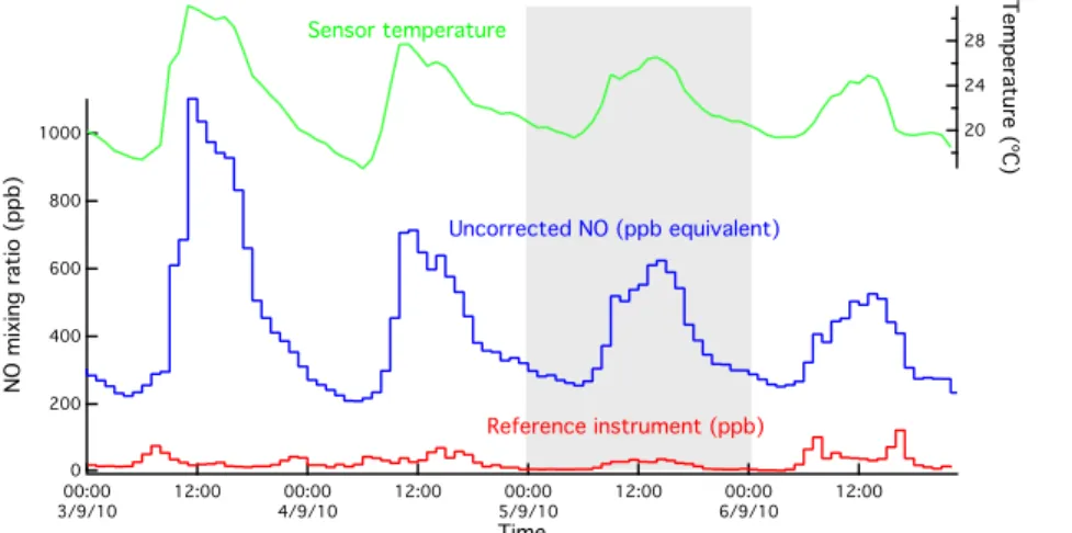
data from a type A1 NO electrochemical cell are shown as ppb equivalent in blue. Also shown, in green, is the instrument temperature. The data in the figure illustrate the importance of temperature effects on the performance of the sensor. See text for further details.
It is clear from the data in Figure 2.6 that there is little correspondence, either in absolute magnitude or diurnal pattern, between the NO mixing ratios measured by the reference instrument and the uncorrected electrochemical sensor data. However, it can be seen that there is a general correlation evident between the uncorrected NO electrochemical measurements and the instrument temperature (which broadly tracks ambient temperature), which is in fact due to the sensor baseline temperature dependence.
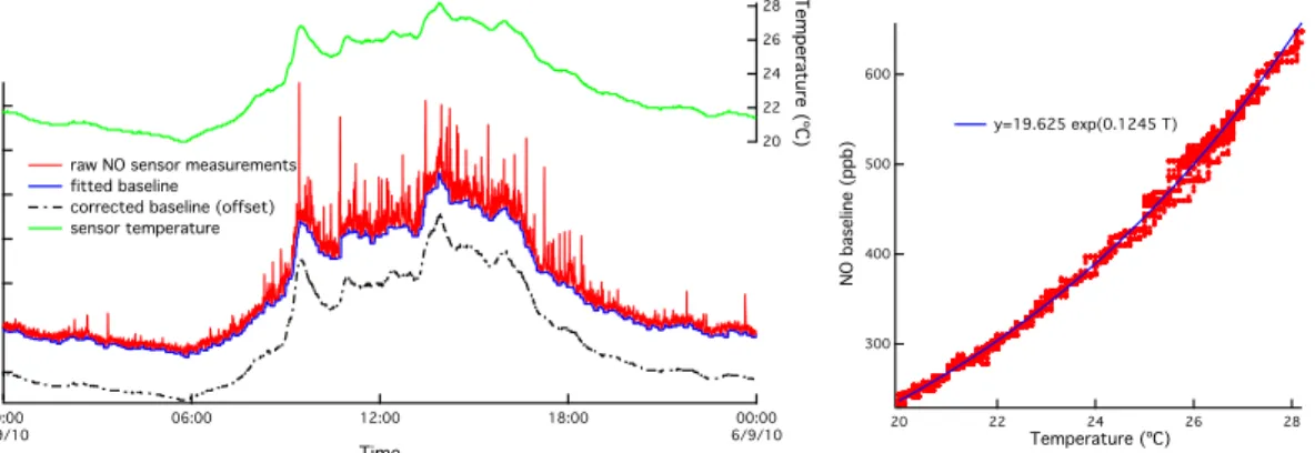
The temperature and RH correction procedure adopted for long-term data sets shown in this study was as follows: a sensor ‘baseline’ was defined for each measurement time t by applying a filter which obtained the minimum measurement encountered within a given time interval of t ± δt. This process was carried out for
a range of values for δt (between 50 and 1750 seconds) so that the optimal value (that which led to the best
fit with temperature) could be used to correct each day of data. Application of this filter process produced curves for each sensor type which reproduced the temperature or RH induce sensor baseline variations. This process, applied to the NO sensor shown in Figure 2.6, is illustrated in Figure 2.7.
Figure 2.7. Correction of baseline temperature effects for a type A1 NO sensor (see text for details) for the 24-hour period shown shaded in Figure 2.6. The left panel shows raw (0.2 Hz) NO data (red), with spikes associated with individual pollution events superposed on a strong diurnal baseline variation, and the fitted baseline (see text) (blue). The right panel shows the exponential relationship between the fitted baseline and instrument temperature (see left panel, green). The temperature correction derived from this temperature-baseline correction is shown in the left panel (black, dashed line), and is offset by 100ppb for clarity.
During the temperature and humidity correction process, either a linear regression or exponential fit (depending on gas species) is obtained between an extracted baseline and the measured instrument temperature. In general over a 24-hour period, atmospheric absolute humidity is found to be approximately constant. Consequently, as relative humidity (RH) changes are therefore largely determined by diurnal temperature changes, the correction process for instrument temperature variations also largely accounts for diurnal changes in RH. The correction process was therefore also adapted to account for absolute (rather than relative) humidity. For the case where the correction factors were linear, temperature and absolute humidity correction constants, corresponding to the baseline change per unit change in temperature (db/dT) and the baseline change per unit change in absolute humidity (db/dH), were derived. This process was repeated for each 24-hour period of data. The data in Figure 2.8 shows that, following this correction, there is excellent agreement between the NO sensor and a reference instrument. The temperature and humidity correction methodology is described in more detail in a paper in preparation (Popoola et al., 2012).
Figure 2.8. Time series (left) and correlation plot (right) of hourly mean NO measurements from a ratified chemiluminescence instrument (red) and an electrochemical sensor corrected for temperature baseline effects (blue – hourly averages; green – 0.2 Hz data). Note the much larger variability evident in the 0.2 Hz data (which is truncated at 200 ppb for clarity). The correlation plot shows the hourly data for the period shown in Figure 2.7 (blue) and the entire period (red), both showing excellent agreement with the reference instrument (see inset equations).
2.5 Long-term sensor stability
The long-term stability of NO sensors can be illustrated using the same data which have been partially shown in Figures 2.6 – 2.8. For each period of data collected over ~ 11 months, hourly averaged NO data measured by a single electrochemical sensor were compared with that from a ratified reference instrument with which it was co-located, allowing gain parameters for the electrochemical sensor to be derived. Assuming the reference instrument to have no instability itself, the sensor gain is stable to within ± 13%, (Figure 2.9), i.e. not significant within the measured errors.
Figure 2.9. Time series of sensor gain for 11 months of NO measurements, calculated by comparison to a reference instrument. The drift in sensitivity/gain is 13% ± 13% (1σ), showing that, within the experimental errors, the stability of the sensor has remained unchanged over the 11-month measurement period. Error bars in the figure represent ± 3σ of the calculated gains for the different periods.
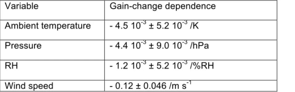
The data obtained during the 11-month period also permit other potential systematic errors to be evaluated. Table 2.2 shows correlations of the sensor gain, derived as described above, in this case with various meteorological parameters. As can be seen, after the temperature/RH correction has been applied as indicated above, there is no significant dependence of sensor gain on either parameter. Similarly, there is no significant dependence on atmospheric pressure (which is to be expected as the devices are intrinsically diffusion-limited (Stetter and Li, 2008)), although, intriguingly, there is a small apparent (negative) dependence on wind speed. The origin of the latter is unclear.
Variable Gain-change dependence Ambient temperature - 4.5 10-3 ± 5.2 10-3 /K Pressure - 4.4 10-3 ± 9.0 10-3 /hPa RH - 1.2 10-3 ± 5.2 10-3 /%RH Wind speed - 0.12 ± 0.046 /m s-1
Table 2.2. Correlations of NO sensor gain with meteorological variables (see text). Errors shown are ± 1 σ.
From the information shown in this section, it can be concluded that, when configured correctly, the electrochemical sensors discussed above respond in a highly linear fashion to ppb levels of their respective target gases. Detection limits are essentially independent of gas concentration but differ for the various gases being sensed. It is also clear, at least on the basis of the laboratory studies, that the intrinsic sensitivity and noise characteristics of the different sensors are compatible with their use in ambient air quality studies. There are clear sensor offset (baseline) dependences on temperature and RH, which depend on sensor type. However, we have demonstrated that temperature/humidity effects on sensor baseline can be accounted for by suitable post-processing of data.
The following section is a description of sensor node design, after which results from a variety of field deployments are presented and discussed.
3. Field Measurements
3.1 Sensor Node Designs
The sensor nodes which were used in these studies are autonomous units incorporating multiple gas sensors, a GPS receiver and a GPRS transmitter, and have integral batteries allowing convenient deployment. The air quality data collected on the devices are firstly labelled by GPS location and time, and are then either stored in situ or transmitted to a central computer server for post-processing and on- or off-line analysis. Although several variants have been constructed, two basic types of sensor nodes were designed to allow both mobile and static deployments.
The mobile sensor nodes were designed to be highly compact and lightweight (see Table 3.1), and thus convenient to carry by volunteers. Electrochemical sensors (usually CO, NO and NO2), along with a
temperature sensor, were mounted behind a mesh opening at one end of the unit (see Figure 3.1), which contained GPS/GPRS modules and batteries. Each node could be operated independently and autonomously, enabling networks to be scaled according to monitoring requirements. This flexibility allowed studies to be carried out in various types of environment, with minimal overheads relating to network design and infrastructure.
Figure 3.1. Mobile sensor unit incorporating three electrochemical sensors (for CO, NO and NO2 in this case). Various
components (GPS/GPRS, batteries etc.) are identified in the left panel. For clarity, the unit is shown without its protective wire mesh, which, during operation, is located in front of the sensors.
The static nodes developed for longer-term studies incorporated larger sensors, with larger electrolyte reservoirs for increased long-term baseline stability, and larger integral batteries allowing operation for in excess of 3 months without intervention. In this case sensors were sealed with rubber O-rings on the bottom of the enclosure behind a protective aluminium bracket (see Figure 3.2) which was also used to mount the unit to lamp posts with suitable bands (see section 4). Temperature and humidity sensors were mounted behind a gas-permeable, hydrophobic membrane on the side of each sensor node.
Figure 3.2. Static sensor unit (or node) plus mounting baseplate. CO, NO, NO2, temperature and relative humidity are
recorded, along with GPS location and time. A view of the open sensor node is also shown (right).
The main differences between the two generations of mobile nodes and the static node, along with other technical specifications, are summarised in Table 3.1.
Mobile Static
Mass Total 445 g 4260 g
Excl batteries 333 g 1430 g
Dimensions 183×95×35 mm 260×177×135 mm
Power 4 × AA NiMH Pb-acid batteries 6 V, 8 Ah,
monobloc
Data storage On board On board
Transmission GPRS (built in) to web server
(Apache 2011 a/b) GPRS (built in) to web server (Apache 2011 a/b)
PIC PIC18F67J10, Microchip
Technology Inc, USA
PIC18F67J10, Microchip
Technology Inc, USA
Firmware PIC chip (PIC18F67J10)
programmed in C
PIC chip (PIC18F67J10) programmed in C
Sensor diameter (mm) 20.2 32.3
Temperature sensor Pt1000 resistance thermometer Pt1000 resistance thermometer
RH sensor N/A Honeywell 4000 series
GPS unit Telit GM862-GPS Telit GM862-GPS
Duration (single charge) Approx. 14hrs, sensing at 5s intervals, 30 min send.
Approx. 3 months, sensing at 10s, sending at 2 hour intervals.
Table 3.1. Outline technical specifications for the mobile and static sensor nodes. 3.2 Sensor Reproducibility
Following the laboratory tests discussed in section 2.2, a number of experiments to verify sensor performance in the field were carried out under typical urban conditions. One such experiment involved mobile sensor units being carried in pairs (2 pairs of sensors each for CO & NO, and NO2)to confirm sensor
reproducibility. This experiment took place over a one-hour period in central Cambridge (UK), during which two volunteers walked on different routes other than for short periods at the start and end of the experiment.
Figure 3.3 shows time series data collected by one pair of sensor nodes co-located for the duration of the experiment. These illustrate the variability in the concentrations of the species measured over small spatial and temporal scales, and confirm that the sensors are responsive at the mixing ratios found in the urban environment. Scatter plots are also shown on the right-hand side, and from these it can be seen that sensor-to-sensor reproducibility is high (R2 values of 0.9532, 0.8361 and 0.9363 for CO, NO and NO2
respectively). Performance is not as repeatable as that in section 2.2 probably due to imperfect co-location of sensor nodes and local mixing effects so that, as a result, one sensor can potentially respond to a brief event slightly differently to its partner. An example of this is shown in the CO time series in Figure 3.3, where at approximately 09:39 am there was a sharp, well defined event which was more evident in sensor A28 than its partner, either owing to its orientation (i.e. A28 was potentially nearer the source) or local micro-scale
mixing. The R2 correlation coefficient is biased accordingly; e.g. removal of data until 0943 yields a slightly improved R2 value of 0.959 for CO. Table 3.2 gives mean values of gradients and a range of R2 values for linear fits generated between electrochemical sensors (two pairs for CO, NO and NO2) sensors paired for the
whole deployment period. These data show how well correlated the sensors are when taking local mixing into account. The Figure and tables were generated from 30-second (for CO and NO2) and 10-second (for
NO) running averages of that collected. Original data were collected at 1 Hz for CO and NO2 and 0.2 Hz for
NO.
Further illustration of the reproducibility of measurements is provided by Figure 3.4, which shows some measurements of CO superimposed on a map of the area over which sensors were carried. Measurements by two volunteers along the same route are seen to differ when data are captured at different times (blue and yellow), but show a strong correlation when the volunteers were co-located (red and green).
Figure 3.3. (Left) Time series plots of CO, NO and NO2 for sensor pairs co-located for the whole deployment period,
and (right) corresponding scatter plots. Data used are a 30-second running average. NO2 data are not corrected for
cross interference with O3 and the likely maximum bias is 24 ppb (equal to the nearest background AURN O3
measurement (Wicken Fen, see section 3.3)).
Table 3.2. Slopes and correlation coefficients for linear fitting equations generated for sensor pairs co-located for an hour-long walk in central Cambridge (UK).
Species Gradient R 2
Pair 1 Pair 2 Pair 1 Pair 2 CO 0.58 0.94 0.86 0.95 NO 0.89 0.91 0.97 0.84 NO2 1.01 1.15 0.95 0.94
Figure 3.4. Selected CO and NO2 measurements from two sensor nodes in parts of central Cambridge superposed on a
road map (map data © 2012 Google). Data from periods during which volunteers walked together are shown in red and green, and those from when they walked apart are shown in yellow and blue. NO2 data not corrected for
interference with O3 (see section 3.3).
The capability of the mobile devices is illustrated graphically in Figure 3.4, in which three-dimensional plots of CO and NO2 are superposed on a road map. Where the devices are co-located in both time and space,
there is excellent correspondence between sensors (see, for example, tables 3.2 and 3.3). However, when at the same location, but now separated in time by even a few tens of seconds, there is little correspondence in observed mixing ratios. This therefore also illustrates very effectively the importance of measurements at the appropriate spatial scales when considering personal exposure in the urban environment.
3.3 Treatment of O3 cross-interferences for NO2 electrochemical sensors.
Two sensor units (CO, NO, NO2) were co-located with the Cambridge City Council (CCC) roadside AURN
site to compare electrochemical sensor measurements of NOx with a calibrated reference instrument. The
reference instrument (Thermo Environmental Model 42C NO-NO2-NOx analyser) was located in the
first-floor offices of the CCC building, with an inlet height of 4m approximately 2.5m horizontally from the kerbside above a busy urban road. Electrochemical sensors (in this case variants of the mobile nodes) were mounted inside a sealed chamber, through which external air was drawn via an inlet placed alongside that of the CCC instrument. As the sensors were indoors, they were exposed to minimal ambient temperature variations (less than ± 0.5oC). Figure 3.5 shows time series data from midnight on the 23rd until 0900 on the 26th of January for NO for the electrochemical and reference instruments. Similarly, data from NO2 sensors
over the same period are compared with the reference instrument in Figure 3.6, before correction for interference with O3.
Figure 3.5. Time series plot for electrochemical NO sensors co-located with a reference instrument at the CCC AURN site. The plots illustrate good agreement between the two techniques for this species.
Figure 3.6. Hourly averaged time series for the NO2 sensors from the same study, uncorrected for the O3 interference
(see text). Also shown is the hourly average O3 mixing ratio from a reference instrument. The two electrochemical
sensors show excellent consistency with each other. However, there is a substantial discrepancy between the uncorrected NO2 data and the reference instrument.
Cross interference with O3 is a significant issue for urban measurements made using the current NO2
sensors, with cross sensitivity for this generation of sensors known to be 100%, making the data, in effect, a measurement of [NO2] + [O3]. At this stage there were no electrochemical measurements of O3 available.
However, O3 measurements were available from the CCC AURN site, and these were therefore used to
correct the NO2 data presented in Figure 3.6. NO2 measurements shown in other figures in the paper are not
corrected for this effect.
Figure 3.7. Time series of NO2 mixing ratios from a reference instrument and from electrochemical sensors, corrected
based on the known O3 cross interference. Agreement between the techniques, over the same period as Figure 3.6, is
significantly improved.
Figure 3.8. Comparison of hourly averaged electrochemical measurements of NO and NO2 (prior to and following
correction of the sensors for the O3 interference) against reference measurements.
Statistical relationships obtained between the NO and NO2 electrochemical cell measurements and the
reference instrument are shown in table 3.3, showing a marked improvement in the agreement for the NO2
measurements once corrected for the O3 interference, although there is still a downward bias of ~ 20%. ECC Sensor NO gain NO R2 NO2 gradient (uncorrected) NO2 gradient (corrected) NO2 R2 1 0.97 ± 0.04 0.80 0.36 ± 0.02 0.81 ± 0.03 0.89
2 1.00 ± 0.06 0.95 0.38 ± 0.02 0.81 ± 0.03 0.92
Table 3.3. Statistics obtained from the inter-comparison of ECC NO and NO2 sensors with reference measurements. The results of this experiment clearly show that the electrochemical sensors used to measure NO and NO2
agree well with established reference techniques for these species, provided that known cross sensitivities are accounted for, although some biases remain for NO2. Development work is in progress to develop NO2
and O3 electrochemical sensors with greater degrees of discrimination and selectivity, and this will be
reported in future papers.
3.4 Mobile Sensor Network Results
Short-term, mobile sensor deployments can provide a representative picture of the rapidly changing and highly granular air quality in an urban area over a deployment period. However, they should not be expected to accurately represent the local air quality over longer timescales (despite collecting 105–106 measurements
over periods of hours), where influences such as meteorology and source morphology become highly significant.
Despite this limitation, though, the “snap-shots” of pollution levels assembled from the data collected do illustrate the large degree of spatial and temporal variability in the concentrations of pollutant gases in different urban environments. The routine measurements currently made by fixed-site monitoring stations, which have intrinsically low spatial resolution when compared with the scales over which chemistry occurs, do not capture many aspects of real variability in urban air quality, as is illustrated below. A more detailed account of this will be given in a separate publication.
Mobile sensors have been used on numerous occasions across a range of different environments in Cambridge, London, Cranfield (all UK), Valencia (Spain), Kuala Lumpur (Malaysia) and Lagos (Nigeria). The largest-scale mobile sensor network deployment to date was in Cambridge and comprised 35 sensor nodes, of which 20 were mobile and measured CO/NO/NO2 and temperature. Units were deployed using
three transport modes (pedestrians, cyclists and drivers), and were also located alongside Cambridge City Council fixed-site monitoring stations. Spatial coverage extended over a 10km-by-10km area, but was weighted towards the heavily trafficked city centre.
Figure 3.9. 3D plots (left to right respectively) of CO, NO and NO2 mixing ratios giving overviews of measurements
obtained during a large, mobile sensor deployment. The peak heights correspond to mixing ratio, with maximum values of 7 ppm, 4.5ppm and 840 ppb for CO, NO and NO2 respectively (map data © 2012 Google and © 2012
Infoterra Ltd & Bluesky).
Visual inspection of Figure 3.9 enables a number of “hotspots” to be identified; these are usually located where traffic density is highest, for example around areas such as the central bus station, on major roads around Cambridge (the A14 and M11 specifically) and in areas where traffic is routinely static (e.g. traffic lights). However, as is discussed below, more sophisticated analysis methods allow more subtle exposure features to be extracted from the data. It should be noted, of course, that while this deployment is an important demonstration of the capabilities of the mobile sensor network philosophy, the fact that measurements were obtained over a short period means that specific features may not be representative of the longer-term environment.
3.4.1 Examples of Individual Exposure
As an illustration of individual exposure, data taken from one sensor node carried by a pedestrian in Cambridge at waist height are shown in Figure 3.10. The mean mixing ratios calculated for this pedestrian sensor node were 515 ppb, 177 ppb and 68 ppb for CO, NO and NO2 respectively. CO data were offset
assuming a natural background mixing ratio of 200 ppb (in line with the initialisation mixing ratios used by Bright et al., (2011)). While the NO2 measurements are strictly [NO2] + [O3] in this case, as background O3
emissions.
There is a broad correlation between the different species (e.g. a minimum around 13.30 with elevated mixing ratios around 13.45 etc.), and clear correlations for some individual pollution events (e.g. most markedly for NO and NO2 at ~ 14.40), although many pollution events, particularly for CO, are not well
correlated with those of the other species. It is noticeable that, in this case, the observed NOx values substantially exceed the average values measured by the neighbouring static sites (operated by the local authority) over the same period; this is one example of fixed monitoring sites not reproducing personal exposure to pollution events. In this case, the average NO2 mixing ratio (68 ppb) was a substantial fraction
of the hourly mean limit for AURN sites (200 µg m-3 or ~100 ppb), while the average measured at the fixed
sites was 16 ppb. The quantitative interpretation of these results is weakened by the fact that the NO2 sensors
were in fact also responding to O3. The analysis method meant that this does not introduce a simple offset by
the background O3, but in fact is likely to slightly underestimate actual NO2 amounts. For future studies,
coupled measurements with NO2 and O3 sensors would resolve this uncertainty.
Figure 3.10. Time series and histograms for a mobile sensor unit carried by a pedestrian as part of a mobile sensor deployment. NO2 data are not corrected for interference with O3 and therefore should be taken to be [O3] + [NO2], i.e.
there may be an additional baseline effect related to response to [O3]. The inset NO Figure shows that the peak at 14.40 exceeded 2.5 ppm. Histograms of the data for NO and NO2 also show, in dotted lines, the average of two
concurrent hourly mean values derived from each of the static sites maintained by the local authority in central Cambridge.
3.4.2 Air quality exposure by transport mode
The data shown in Figure 3.9 can be disaggregated to describe exposure in a variety of different ways, including differences among individuals and across different transport modes. In Figure 3.11 are shown time series and measurement histograms of carbon monoxide from several sensor nodes obtained in central Cambridge as part of the mobile sensor deployment. The data show the widely different air quality environments encountered by individuals, with a suggestion (see the histograms) that, for example, vehicle occupants are exposed to systematically higher values of carbon monoxide.
Figure 3.11. Time series and measurement histograms of carbon monoxide, obtained from a number of sensor nodes deployed in central Cambridge (UK) as part of a large, mobile sensor network. Measurements made by pedestrians and cyclists are shown in green and red respectively, with in-vehicle measurements shown in blue. For clarity, the abscissae of the histograms are on a single scale.
As sampling was carried out in broadly the same area, the means are similar between the pedestrians and cyclists, but these are both lower than that for the drivers. Cyclists were generally exposed to slightly higher concentrations than pedestrians, probably owing to the relative road positions of the volunteers i.e. cyclists were closer to the stream of traffic, the primary local emission source for these species.
Figure 3.12. Normalised probability distributions of CO, NO and NO2 mixing ratios obtained during the Cambridge
deployment, disaggregated by transport mode.
Figure 3.12 shows probability distributions of CO, NO and NO2 mixing ratios disaggregated by transport
mode taken from the 3-hour mobile deployment. Given the ‘snapshot’ nature of the study, some caution must be applied to their interpretation. However, at face value, it seems that vehicle occupants are exposed to significantly higher CO and NO concentrations than cyclists or pedestrians, while pedestrians appear to
be exposed to a higher NO2 tail in the distribution. The data on vehicle exposure are, however particularly
limited owing to the fact that data from only 2 vehicles were used (c.f. 8 pedestrians, 10 cyclists). An additional factor to consider is that while the sensors provide information on exposure, they take no account of different levels of physical activity, leading to potentially differing dosages for similar exposures.
3.4.3 Air quality measurements in Cambridge, Valencia and Lagos
As a further illustration of the mobile sensor node capability, Figure 3.13 shows normalised fractions obtained during short-term deployments in Cambridge (UK), Valencia (Spain) and Lagos (Nigeria). Subject to caveats about representativeness, there are clear indications of differences in all three species, most notably between Lagos and the European cities. The fact that these data may be gathered in such diverse locations with little to no infrastructure overheads illustrates the ease with which units may be deployed. A major implication of these studies is the potential application of the mobile sensor nodes in studies involving exposure assessment for the purpose of providing the necessary pollution data for epidemiological studies.
Figure 3.13. Normalised fractional exposure obtained during short-term deployments in Cambridge (UK), Valencia (Spain) and Lagos (Nigeria) using the mobile sensor nodes discussed in section 3.1.
4.0 Long-term, Static Networks
A network of static sensor nodes (see section 3.1) was deployed in the Cambridge area for a period of approximately 2.5 months from 12th March to 26th May 2010. In total, 46 static sensor nodes were deployed, 21 of which were in central Cambridge. This is significantly denser than the existing infrastructure (five monitoring sites in Cambridge, one of which is a roadside AURN site monitoring NOx) and the data
gathered provide a far more detailed assessment of the local urban environment over the period of deployment. Each sensor node was installed at a height of 3 m on selected lamp-posts around Cambridge and South Cambridgeshire, with node locations as shown in Figure 4.1.
Figure 4.1. Static sensor node locations used for the Cambridge static deployment (left), with typical lamppost mounting (photograph right) (Map data © 2012 Google).
This deployment generated a large number of measurements (excluding NO2 measurements, over
90,000,000 measurements including CO, NO, RH and temperature) which will be discussed in detail in a number of subsequent papers. A subset of data from the deployment campaign is presented here to illustrate the capability of the sensor network approach. In Figure 4.2 are shown several time series of CO mixing ratios obtained from a single, inner-city electrochemical sensor node during this campaign. The uppermost
panel (a) shows the complete 2.5-month time series, with a large number of individual pollution events superposed on a generally varying background. At this resolution any diurnal pattern is masked, although there are significant differences which are likely to be linked to synoptic weather patterns and, in particular, planetary boundary layer height and venting. Panel b) shows a single month (April) when again there is significant meteorologically linked variability, but where a diurnal periodicity is now beginning to be seen. Panel c) shows a single week (16-23rd April) where not only is the diurnal periodicity clearly apparent, but now sub-diurnal features related to traffic flow are seen. Panel d) shows a single day (20th April) where individual pollution events are now apparent, superposed on the morning and evening traffic peak densities.
Figure 4.2. Time series showing CO measurements from an inner-city electrochemical sensor node for the deployment duration (a), together with subsets of one-month, one-week and one-day periods (b) – d) respectively) from a selected sensor node. All measurements are 30-second averages.
An example of the statistical information contained in these measurements is shown in Figure 4.3 (generated using the OpenAir open source air quality analysis tool (OpenAir 2010)), where clear diurnal signatures in all species are now apparent, together with the longer time-series variability and the ‘weekend’ effect.
Figure 4.3. Time series plots, averaged over different time scales, of hourly CO electrochemical sensor concentrations at the LAQN station in Gonville Place, Cambridge. The shading represents 95% confidence interval about the mean for each plot.
Figure 4.4. Selected time series and bivariate polar plots for daytime carbon monoxide measurements obtained during a 2.5-month deployment of lamppost-mounted sensor nodes, as described in section 4, in the Cambridge area, illustrating typical variability (see text for further discussion). Time series plots have identical ordinate scales. Bivariate plots are also on identical scales, with the exception of the central Cambridge site (bottom right) which, for clarity, has a different colour scale. Cambridge meteorological data is courtesy of the University of Cambridge Computer laboratory Digital Technology Group.
The capability of the high density fixed site network is illustrated by the data shown in Figure 4.4, which shows time series and bivariate polar plots for daytime carbon monoxide obtained from a 2.5-month deployment of static sensor nodes (see section 4) illustrating the range of conditions encountered in the urban and sub-urban areas associated with differing emission rates. Also apparent are increases associated with increased proximity to linear road sources (most notably in the top figures) where elevated concentrations occur when the wind direction is oriented parallel to the road. Although the details apparent are beyond the scope of this paper, the capability of the sensors for monitoring over extended periods as parts of dense networks is clear.
5. Discussion and conclusion
In this paper, we show that, operated suitably, CO, NO and NO2 electrochemical sensors can provide
parts-per-billion (~ µg m-3) level mixing ratio sensitivity with low noise and high linearity, making them suitable
for urban air quality measurements. The sensors are generally highly selective, although there emerged from this work some cross-sensitivities e.g. between O3 and NO2 sensors; in future work, these will be catered for
through the use of multiple sensors.
When operated in the field, the sensors show baseline (zero) signals which depend significantly (although differently for different sensor types) on ambient temperature and relative humidity. Of the sensor types investigated, this is most apparent for NO, and a post-processing procedure is presented which eliminates this effect, yielding excellent agreement with reference AURN instruments where measurements are available (NO and NO2). Selected results also show that the sensors can be operated without significant gain
attenuation over long periods (up to 12 months thus far), with the expectation of operable lifetimes of several years without replacement.
communication) have also been constructed for deployments as parts of mobile and static air quality sensor networks capable of sending real-time air quality data to a central server for processing and display.
Low-cost (~£100s) mobile and static networks of over 40 nodes have been successfully deployed, with results in the paper demonstrating the feasibility of high-density and scalable sensor networks for a variety of periods thus far up to 2.5-months. Results from these deployments shown in the paper have provided views of urban air quality segregated by, for example, transport mode and personal exposure. These data have a measurement density (in both space and time) which is unachievable using current standard measurement methods.
Overall, this work has demonstrated the potential of low-cost sensor network systems for air composition measurements in the urban environment, and to be capable of doing so at an appropriate granularity (and cost) to quantify airborne pollution levels on local scales. Such systems have been shown to be capable of producing high spatial and temporal resolution measures of pollution levels which could contribute to scientific understanding, as well as addressing economic, policy and regulatory issues spanning climate change, air quality and human exposure (and health) responses.
While it has been shown that post-processing and artefact removal are required to achieve results, the key conclusion is that low-cost miniature sensors previously considered at best indicative can, when suitably operated, be used for fully quantitative measurements of urban air quality. This work shows that low-cost air quality sensor networks are now feasible for widespread use for monitoring at ambient levels, complementing other measurement methodologies, and are now rapidly emerging as a feasible measurement technique for inclusion in air quality monitoring and regulation, source attribution and human exposure studies.
Improvements in sensor technologies are currently emerging and, for example, the inclusion of other gaseous species (e.g. O3, SO2), and suitable particulate monitors can only strengthen the case for their
increasing use in assessing the scientific, health and legislative implications of urban air quality.
Acknowledgements
The authors would like to thank the following: Cambridge City Council for their cooperation in conducting these studies; O2 for provision of hardware such as mobile phones and SIM cards used in the transmission of
data; Brian Jones of the Digital Technology Group, University of Cambridge Computer Laboratory for meteorological data. The authors would also like to thank DfT and EPSRC for funding for the MESSAGE project.
References
Abelsohn, A., Sanborn, M. D., Jessiman, B. J., Weir, E. Identifying and managing adverse environmental health effects: 6. Carbon monoxide poisoning. Canadian Medical Association Journal. Vol 166. 13. 1685-1690. Jun 2002.
Austin, C., Roberge, B., Goyer, N. Cross-sensitivities of electrochemical detectors used to monitor worker exposures to airborne contaminants: False positive responses in the absence of target analytes. J. Environ. Monit. 8, 161–166, 2006.
Bard, A.J., Faulkner, L.R., Electrochemical Method: Fundamentals and Application. 2nd ed. New York: John Wiley & Sons, 2001.
Bright, V., Bloss, W., Cai, X. Modelling atmospheric composition in urban street canyons. Weather., 66, 4, 106-110, DOI: 10.1002/wea.781, 2011.
Grant, A., Stanley, K. F., Henshaw, S. J., Shallcross, D. E., O’Doherty, S. High-frequency urban measurements of molecular hydrogen and carbon monoxide in the United Kingdom. Atmos. Chem. Phys., 10, 4715–4724, 2010.
Health Effects Institute. Traffic-Related Air Pollution: A Critical Review of the Literature on Emissions, Exposure, and Health Effects A Special Report of the HEI Panel on the Health Effects of Traffic-Related Air Pollution. Special Report 17. January 2010.
Hitchman, M. L., Cade, N. J., Gibbs, K. T., Hedley, N. J. M. Study of the Factors Affecting Mass Transport in Electrochemical Gas Sensors. Analyst, 122, 1411-1418. DOI: 10.1039/A703644B. 1997.
Lehr, E. L. Carbon monoxide poisoning: a preventable environmental hazard. Am J Public Health Nations Health. 60. 2. 289–293. Feb 1970.
McConnell, R., Islam, T., Shankardass, K., Jerrett, M., Lurmann, F., Gilliland, F., Gauderman, J., Avol, E., Kuenzli, N., Yao, L., Peters, J., Berhane, K. Childhood Incident Asthma and Traffic-Related Air Pollution at Home and School. Environmental Health Perspectives. Vol 118. 7. 1021-1026. Jul 2010.
Ropkins, K., Colvile, R. N. Critical Review of Air Quality Monitoring Technologies for Urban Traffic Management and Control (UTMC) Systems. Urban Traffic Management & Control (UK). November 2000. World Health Organisation. Air Quality Guidelines for Europe, second edition. WHO Regional Publications No. 91, ISBN 92 890 1358 3. 2000.
World Health Organisation. Air quality guidelines for particulate matter, ozone, nitrogen dioxide and sulfur dioxide. Global update 2005. Summary of risk assessment. WHO/SDE/PHE/OEH/06.02. 2006.
Stetter, J., Li, Jing. Amperometric gas sensors - A review. Chem. Rev. 108, 2, 352−366, DOI: 10.1021/cr0681039, Feb 2008.
Lee, JD., Lewis, AC., Monks, PS., Jacob, M., Hamilton, JF., Hopkins, JR., Watson, NM., Saxton, JE., Ennis, C., Carpenter, LJ., Carslaw, N., Fleming, Z., Bandy, BJ., Oram, DE., Penkett, SA., Slemr, J., Norton, E., Rickard, AR., Whalley, LK., Heard, DE., WJ., Gravestock, T., Smith, SC., Stanton, J., Pilling, MJ., Jenkin, ME. Ozone photochemistry and elevated isoprene during the UK heatwave of august 2003.
Atm. Env. 40, 7598–7613, DOI: 10.1016/j.atmosenv.2006.06.057, Dec 2006.
Hamann, C., Hamnett, A., Vielstich, W. Electrochemistry. 2nd Edition. Wiley-VCH. ISBN: 978-3-527-31069-2. 2007.
Popoola, O.A.M., Mead, M.I., Stewart G. B. and Jones, R.L. Development of Baseline-Temperature Correction Methodology for Electrochemical Sensors, and Implications of this Correction on Long-Term Stability. In preparation (2012).
Apache HTTP Server Project. http://httpd.apache.org/. Searched Nov 2011. 2011a.
Apache HTTP Server 2.2 Official Documentation", volumes 1 – 4. http://httpd.apache.org/docs/2.1 Searched Nov 2011. 2011b.
Carslaw, D. C., Ropkins, K. Openair - an R package for air quality data analysis. Environmental Modelling & Software. In press. 2011. http://www.openair-project.org/Downloads/Reports.aspx. Searched Nov 2011. Defra. http://uk-air.defra.gov.uk/networks/network-info?view=aurn. Searched Nov 2011. 2011.
Environment Canada. http://www.ec.gc.ca/rnspa-naps/Default.asp?lang=En&n=5C0D33CF-1. Searched Nov 2011. 2011.