Private Retirement Savings in Germany: The
Structure of Tax Incentives and Annuitization
H
ANS
F
EHR
C
HRISTIAN
H
ABERMANN
CES
IFO
W
ORKING
P
APER
N
O
.
2238
CATEGORY 1: PUBLIC FINANCE
MARCH 2008
An electronic version of the paper may be downloaded
• from the SSRN website: www.SSRN.com
• from the RePEc website: www.RePEc.org
CESifo Working Paper No. 2238
Private Retirement Savings in Germany: The
Structure of Tax Incentives and Annuitization
Abstract
The present paper studies the growth, welfare and efficiency consequences of the recent introduction of tax-favored retirement accounts in Germany in a general equilibrium overlapping generations model with idiosyncratic lifespan and labor income uncertainty. We focus on the implicit differential taxation of specific savings motives, the mandatory annuitization of benefits and the impact of special provisions for low-income households. The simulations indicate that the reform improves overall economic efficiency by about 0.6 percent of aggregate resources, but welfare decreases significantly for future generations. Finally, we show that special provisions could be very effective in raising the participation of low-income households despite their low budgetary cost.
JEL Code: H55, J26.
Keywords: individual retirement accounts, annuities, stochastic general equilibrium.
Hans Fehr Department of Economics University of Wuerzburg Sanderring 2 97070 Würzburg Germany hans.fehr@uni-wuerzburg.de Christian Habermann Department of Economics University of Wuerzburg Sanderring 2 97070 Würzburg Germany February 2008
Previous versions of the paper were presented at conferences and workshops in Garmisch, Mannheim, Utrecht and Wuppertal. We thank Peter Broer, Anette Reil-Held, Kerstin Schneider, Øystein Thøgersen and other seminar participants for helpful comments and Fabian Kindermann for providing excellent research assistance. Financial support from the Forschungsnetzwerk Alterssicherung (FNA) of the Deutsche Rentenversicherung Bund is gratefully acknowledged.
1
Introduction
As many other OECD countries before, Germany has introduced a program to promote the development of private pensions savings in 2001. The so-called “Riester pensions”(named after the former secretary of work Walter Riester) are intended to compensate for the phased-in cuts in future public pensions. In principle, the program design is very similar to individual retirement accounts (IRAs) in the US or the United Kingdom. Contributions to these accounts up to a certain contribution limit are voluntary, withdrawal before retirement is restricted, and the savings are tax deferred. Therefore, contributions are tax deductible, the accrued return on investment is tax exempt, but the pension benefits arising from these savings are fully taxed. However, three specific features distinguish the German reform design from the implementation of IRAs in other countries. First, preferential tax treatment of old-age savings is partly financed by an increased taxation of other savings. Second, the program mandates annuitization of the accounts at the time of retirement. Finally, the program provides a direct subsidy which depends on the actual family status and is very generous especially for low-income households with children. The present paper attempts to quantify the efficiency and distributional consequences of the German Riester accounts. The efficiency effects of the program originate from the differential taxation of saving motives and the implicit provision of a longevity insurance. As Nishiyama and Smetters (2005) have shown, it is not efficient to eliminate the taxation of capital income in a model with labor income uncertainty. Implicitly, capital income taxation acts as an insurance device in such a model which improves economic efficiency. However, uniform taxation of all savings might also not be efficient. Since precautionary savings appear to be less sensitive to changes in the after-tax rate of return than life cycle savings (see Cagetti (2001) or Bernheim (2002, 1199)), an optimal tax structure would tax life cycle savings at a lower rate than precautionary savings. The reduced taxation of savings in retirement accounts could be interpreted as a means to separate the two savings motives. Since accounts are illiquid before retirement, only life cycle savings are allocated there, while precautionary savings are allocated in liquid savings accounts. The mandatory purchase of private life annuities at retirement also has efficiency implications. It is proposed in order to shelter participants against the risk of outliving their assets. When private annuity markets are absent, mandatory annuitization overcomes this market failure and increases aggregate efficiency, see Fehr and Habermann (2008).
The distributional effects of the program work in two directions. First, mandatory an-nuitization redistributes implicitly from future to existing generations since it reduces unintended bequest. Pecchenino and Pollard (1997) show that the bequest reduction
de-creases long-run capital accumulation and growth in an endogenous growth model. Fehr and Habermann (2008) demonstrate in an exogenous growth model that future gener-ations will be hurt by annuitization, if the interest rate is sufficiently higher than the growth rate. In the latter case the bequest reduction dominates the benefits from the insurance provision. Second, due to the special provisions for low- and medium-income savers we are also interested in the distributional implications within a cohort. The ques-tion is here whether the special provisions are effective in increasing the participaques-tion of low- and medium-income households. The answer to this question also determines the effectiveness of the policy to create new savings. As indicated by Benjamin (2003), savings incentives have a significant stronger impact among low-income savers whereas contributions by high-income households are more likely to represent funds shifted from existing savings. In addition, given the progressive income tax system, the budgetary cost of traditional IRA schemes are likely to rise with the income of participants although the effectiveness may well be declining. Consequently, traditional tax deferral is often considered as an expensive means of encouraging additional saving, see the discussion in Bernheim (2002) and OECD (2004).
In order to quantify the efficiency and distributional consequences of the German Riester accounts, we apply a general equilibrium overlapping generations model in the Auerbach-Kotlikoff (1987) tradition which includes mortality and individual income risk as well as borrowing constraints. Private annuity markets are closed by assumption, but the public sector provides partial insurance via the progressive tax system and the unfunded pension system.1 ˙Imrohoro˘glu et al. (1998) evaluate in this framework the long-run consequences of IRAs on the US capital stock for various contribution limits and tax savings instruments. They conclude that about 9 percent of IRA contributions during the 80ies constituted additional savings which raised the US capital stock by about 6 percent. Fuster et al. (2005) extend their framework by introducing mandatory retirement accounts into a model with two-sided altruism where individual life expectancy and income are positively correlated. Their study either eliminates the existing system or substitutes halve of the contributions by mandatory savings in private accounts which are either annuitized or not. While the long-run capital stock increases in all reform scenarios, the mandatory saving programs outperform the full privatization policy in terms of long-run capital and consumption growth.
The present study complements Fehr et al. (2008) who also analyze alternative IRA options for Germany. Compared to the US studies, wo do not only compare steady states,
but compute the complete transition to the new long-run equilibrium in order to quantify the intergenerational welfare consequences. After compensating existing households with lump-sum transfers, we are also able to isolate the overall efficiency consequences of the policy reform. In addition, we include a progressive tax and subsidy system in order to capture the intragenerational implications of the reform. Finally, our model assumes a specific individual preference structure that allows to distinguish the effects of risk aversion and intertemporal substitution.
Our simulations indicate three central results. First, the reform increases economic effi-ciency by roughly 0.6 percent of aggregate resources. The effieffi-ciency gain is mostly due to the fact that the reform improves the insurance properties of the tax system and allows to tax different savings motives separately. Second, despite the significant gains in aggre-gate efficiency, future generations are most likely hurt by the reform due to the reduction of accidental bequest. In our benchmark calibration, long-run welfare decreases by 0.68 percent of lifetime resources. The welfare losses are stable for a wide range of parame-ter combinations. Third, the study indicates that the special provisions for low-income households are successful in increasing the participation of this group, but they may have a negative side effect on labor supply.
The next section describes the modeling of the German savings incentive scheme. Then we sketch the structure of the simulation model. Section four explains the calibration and simulation approach. Finally, section five presents the simulation results and section six offers some concluding remarks.
2
Saving incentives for low-income individuals
In order to highlight the central effects of Riester accounts, the modeling of their cen-tral elements is highly stylized. Our simulation model simplifies withdrawal restrictions and the annuitization requirement and ignores all transitional provisions for the phase-in period between 2002 and 2008.2 In order to highlight the very special provisions for low-income individuals, Table 1 compares the benefits from traditional IRAs and from the German system. The left column shows the gross income level of a contributor. As in Germany it is assumed that contributions (s) amount to 4 percent of gross income up to the contribution limit (ˆs) of 2100 e. The third column reports the marginal tax rate in Germany in year 2005 for a one-earner-couple when the income splitting method 2A detailed discussion of the institutional arrangements, the transitional provisions, the changes after 2005 and the recent development of Riester accounts is provided in B¨orsch-Supan et al. (2007).
Table 1: Benefit payments with alternative saving incentives (in e)
Gross IRA Marginal Traditional Direct German
income contribution tax rate IRA scheme saving system
(in %) (2)×(3) subsidy max[(4),(5)]
(1) (2) (3) (4) (5) (6) 10.000 400 0 0 350 350 20.000 800 19 152 350 350 30.000 1200 25 300 350 350 40.000 1600 27 432 350 432 50.000 2100 30 630 350 630 75.000 2100 35 735 350 735 100.000 2100 41 861 350 861
is applied. Column (4) computes the typical benefit in a traditional IRA scheme where contributions could be deducted from the tax base. Due to the rising marginal tax rate, the subsidy rate increases with income so that high-income individuals have a stronger in-centive to contribute. The German system also allows such a tax deduction, but provides in addition a direct subsidy (ds) which depends on the family status. If the contribution is at least 4 percent of income, the saving subsidy consists of a basic subsidy of 154e per adult and an additional child subsidy of 185 e. Consequently, a family with two children could receive about 350 e per adult, as shown in column (5). As in the last column, tax authorities in Germany automatically compute whether the direct subsidy or the tax allowance is optimal for the considered tax payer. Consequently, the German subsidy system offers strong incentives for low- and medium-income families with children. Of course, the above calculations only serve illustrative purposes. In the simulation model we first compute the advantagedaj of direct subsidies compared to tax deductions at age
j from daj(yj, sj) = max £ dsj −(T(yj,0)−T(yj, sj)),0 ¤ (1) where T(yj, sj) = T05 ¡ yj −min[sj,sˆ] ¢ (2) computes individual income tax payments. The function T05(·) defines the marginal tax schedule in Germany in year 2005 (inclusive solidarity surcharge) and yj denotes taxable
income at age j. Direct subsidiesdsj are zero for traditional IRAs, so that the advantage
daj is zero as well. For the German system we define
dsj = min · min · sj 0.04wj ,1 ¸ trj,0.9sj ¸ . (3)
This function includes the fact that direct subsidies are proportionally reduced if the contributions are below 4 percent of annual incomewj. The hump-shaped, age-dependent
transfer schemetrj tries to capture the changing family status over the life cycle. At age
20-24 transfers start at 200 e, then they increase linearly until they peak at 350 e at age 35-44 and decline again afterwards. However, direct subsidies are not allowed to exceed individual contributions. Therefore, a minimum saving amount is specified which depends on the family status. For simplicity, we assume in the following that 10 percent of contributions have to be at least financed from own resources.
In order to eliminate the liquidity of retirement accounts during employment and avoid positive contributions after retirement, the function
φj(sj) = sj if j < jR and sj ≤0 daj if j < jR and sj >0 −∞ if j ≥jR and sj >0 0 else. (4)
is added to the budget constraint (8). Consequently, before retirement (i.e. at agej < jR)
withdrawals from IRAs are not possible, since all the money would be lost.3 On the other hand, positive contributions could induce a public transfer daj before retirement and a
prohibitive penalty if they are made after retirement.
3
The model economy
3.1
Demographics and intracohort heterogeneity
We consider an economy populated by overlapping generations of individuals which may live up to a maximum possible lifespan of J periods. At each date, a new generation is born where we have normalized its size N1 = 1, i.e. we assume zero population growth. Since individuals face lifespan uncertainty with ψj < 1 the time-invariant conditional
survival probability from age j−1 to age j, i.e. Nj =ψjNj−1 and ψJ+1 = 0.
Our model is solved recursively. Consequently, an agent faces the state vector zj =
(j,aj,aRj, epj, ej) where j ∈ J = {1, . . . , J} is the household’s age, aj ∈ A = [a¯,¯a]
denotes (liquid) assets held at the beginning of agej, aR
j ∈R = [a¯R,¯aR] denotes assets in
individual retirement accounts held at the beginning of age j, epj ∈P = [ep, ep] defines
the agent’s accumulated earning points for public pension claims and ej ∈Ej = [ej, ej] is
the individual productivity at age j.
Since income is uncertain the productivity state is assumed to follow a first-order Markov process described in more detail below. Consequently, each age-j cohort is fragmented into subgroups ξ(zj), according to the initial distribution (i.e. at j = 1), the Markov
process and optimal decisions. Let X(zj) be the corresponding cumulated measure to
ξ(zj). Hence, Z
A×R×P×Ej
dX(zj) = 1 for all j = 1, . . . , J
must hold, asξ(zj) is not affected by cohort sizes but only gives densities within cohorts.
In the following, we concentrate on the long-run equilibrium and omit the time indextand the state indexzj for every variable whenever possible. Agents are then only distinguished
according to their agej.
3.2
The household side
Our model assumes a preference structure that is represented by a time-separable, nested CES utility function. In order to isolate risk aversion from intertemporal substitution, we follow the approach of Epstein and Zin (1991) and formulate the maximization problem of a representative consumer at age j and state zj recursively as
V(zj) = max `j,cj,sj ½ u(cj, `j)1− 1 γ +δ · ψj+1E[V(zj+1)]1− 1 γ + (1−ψ j+1)µq 1−γ1 j+1 ¸¾ 1 1−1γ (5) with E[V(zj+1)] = "Z Ej+1 π(ej+1|ej)V(zj+1)1−ηdej+1 # 1 1−η . (6)
In (5) the variables `j, cj and qj+1 denote leisure, consumption and bequest at age j, respectively. The parameters δ and γ represent the discount rate and the intertempo-ral elasticity of substitution between consumption in different years while µ defines the strength of the bequest motive. Since lifespan is uncertain, the expected utility in future periods is weighted with the survival probabilityψj+1. Productivityej at each agej is
un-certain and depends on the productivity in the previous period. Consequently,π(ej+1|ej)
in (6) denotes the probability to experience productivity ej+1 in the next period if the current productivity is ej. The parameter η defines the degree of (relative) risk
aver-sion. Note that for the special case η = 1
γ we are back at the traditional expected utility
specification, see Epstein and Zin (1991, 266). The period utility function is defined by
u(cj, `j) = h (cj)1− 1 ρ +α(` j)1− 1 ρ i 1 1−1ρ (7)
where ρ denotes the intratemporal elasticity of substitution between consumption and leisure at each age j. Finally, the leisure preference parameter α is assumed to be age independent.
The budget constraint is defined as follows:
aj+1 = aj(1+r)+wj+pj+bj+vj−τmin[wj; 2 ¯w]−sj−[T(yj, sj)−φj(sj)]−(1+τc)cj (8)
with a1 = 0 and aj ≥ 0∀j. In addition to interest income from savings raj, households
receive gross labor incomewj =w(1−`j)ej during their working period as well as public
pensions pj during retirement. As time endowment is normalized to one, 1−`j defines
working time and w the wage rate for effective labor. They may receive (accidental) bequestsbj and in some simulations they receive (or have to finance) compensation
pay-ments vj which are explained below. During employment, they contribute to the public
pensions system but only up to the contribution ceiling which amounts to the double of average income ¯w. They also contribute to or withdraw from retirement accounts sj
and have to pay progressive income taxes T(·) where in some cases the direct subsidies are subtracted. All remaining income is used for consumption where the consumer price includes consumption taxes τc.
Retirement account assets accumulate according to aR j+1 = aRj(1 +rj) + min[sj,sˆ] with rj = 1 +r max[ωj, ψj] −1 (9) where aR
1 = 0 and aRj ≥0∀j. Without annuitization at agej, we set ωj = 1, so that the
survival probability ψj has no effect on the individual return, i.e. rj = r. If retirement
account assets are annuitized at age j, we set ωj = 0, so that the periodic returns are
annuitized, i.e. rj > r. Note that contributions cannot exceed the contribution limit ˆs.
After retirement (i.e. j ≥jR and sj ≤0) we have to distinguish two cases: First, without
mandatory annuitization, retired households can decide how much to withdraw. Second, with mandatory annuitization, retirees receive a fixed benefit depending on their wealth at the beginning of retirement aR
jR: sj =− (1 +rjR)aRjR PJ j=jRΠ j i=jR+1(1 +ri) −1. (10)
Our model abstracts from other annuity markets. Consequently, private assets and non-annuitized retirement account assets of all agents who died are aggregated and then distributed among all working age cohorts following an exogenous age- and productivity-dependent distribution scheme Γj(ej), i.e.
bj = Γj(ej) J X i=1 (1−ψi+1)Ni Z A×R×P×Ei qi+1(zi)dX(zi) for all j = 1, . . . , jR−1, (11)
whereqi+1(zi) = (1 +r)[ai+1(zi) +ωi+1aRi+1(zi)(1−τb)]. The age distribution of bequests
is computed in the initial steady state where we assume that the heirs always receive the assets of the generation which was 25 years older. Since bequest can be received only during employment, we adjust this rule at the beginning and at the end of employment. Within a generation bequests are distributed proportional to the current productivity level ej, which highlights their stochastic nature and also reflects empirical evidence.4
Finally, inheritances from IRAs are due to a specific inheritance tax τb since they were
accumulated tax free.5
3.3
The production side
Firms in this economy use capital and labor to produce a single good according to the Cobb-Douglas production technology Y = %KεL1−ε where Y, K and L are aggregate
output, capital and labor, ε is capital’s share in production, and % defines a technology parameter. Capital depreciates at a constant rate δk and firms have to pay corporate
taxes Tk = τk
£
Y −wL−δkK
¤
where the corporate tax rate τk is applied to the output
net of labor costs and depreciation. Firms maximize profits renting capital and hiring labor from the households so that the marginal product of capital net of depreciation and corporate taxes equals the market interest raterand the marginal product of labor equals the wage ratew for effective labor.
3.4
The government sector
Our model distinguishes between the tax system and the pension system. In each period the government issues new debt ∆B and collects taxes from households and firms in order to finance general government expenditures G as well as interest payments on its debt. Whereas government purchases of goods and services G are fixed per capita, we assume a constant debt to output ratio of 60 percent in the benchmark case. Consequently, the long-run equilibrium (i.e. where ∆B = 0) government budget is defined by
G+rB=Ty +τcC+Tb+Tk, (12)
4De Nardi (2004) highlights the link between individual productivity and inheritance. Fehr et al. (2008) also report the consequences of alternative bequest distributions.
5If account owners in Germany die before retirement, their heirs have to pay back all the tax benefits received in former periods if the wealth is not transferred to another retirement account.
where C defines aggregate consumption (see equation (20)) and revenues of income and bequest taxation are computed from
Ty = J X j=1 Nj Z A×R×P×Ej [T(yj(zj), sj(zj))−φj(sj(zj))]dX(zj) and Tb =τb J X j=1 Nj Z A×R×P×Ej ωj+1(1−ψj+1)(1 +r)aRj+1(zj)dX(zj).
We assume that contributions to public pensions are exempted from tax while the benefits are fully taxed. Consequently, taxable gross income yj is computed from gross labor
income net of pension contributions and a fixed work related allowance dw, nominal6
capital income net of a saving allowanceds and - after retirement - public pensions
yj = max[wj −τmin[wj; 2 ¯w]−dw; 0] + max[˜raj−ds; 0] +pj. (13)
Note that we do not include interest income from retirement accounts.
The pension system pays old-age benefits and collects payroll contributions from wage income below the contribution ceiling which is fixed at two times the average income ¯w. Individual pension benefits pj of a retiree of age j ≥ jR in a specific year are computed
from the product of his earning pointsepjR the retiree has accumulated at retirement and the actual pension amount (AP A) of the respective year:
pj =epjR ×APA. (14)
In each year of employment, the worker receives an earning point depending on his relative income positionwj/w¯up to the contribution ceiling. Since the latter is fixed at the double
of average income ¯w, the maximum earning points that could be collected per year are 2. Accumulated earning points at age j are therefore
epj+1 =epj + min[wj/w¯; 2], (15)
with ep1 = 0.
The budget of the pension system must be balanced in every period. Consequently, the general contribution rateτ is computed from
τ = PJ j=jRNj R A×R×P×Ejpj(zj)dX(zj) PjR−1 j=1 Nj R A×R×P×Ejmin[wj(zj); 2 ¯w]dX(zj) . (16)
6In order to reflect realistic features of capital income taxation in a model without inflation, we assume for taxation purposes a nominal interest rate ˜r, i.e. real interest raterplus a fictive inflation of two percent per year. The latter exacerbates the distortions ofreal capital income taxation, see Feldstein (1997).
3.5
Equilibrium and the computational method
Given the fiscal policy {G, B, T05(.), τb, τc, τk, τ, φ, ω,sˆ}, a stationary recursive
equilib-rium is a set of bequests {b(zj)}Jj=1, value functions {V(zj)}Jj=1, household decision rules
{cj(zj), `j(zj), sj(zj)}Jj=1, time-invariant measures of households {ξ(zj)}Jj=1 and relative prices of labor and capital {w, r} such that the following conditions are satisfied:
1. given fiscal policy, factor prices and bequests, households’ decision rules solve the households decision problem (5);
2. factor prices are competitive, i.e.
w = (1−ε)% µ K L ¶ε (17) r = (1−τk) " ε% µ L K ¶1−ε −δk # (18) 3. in the closed economy aggregation holds,
L = X j Nj Z A×R×P×Ej (1−`(zj))ejdX(zj) (19) C = X j Nj Z A×R×P×Ej cj(zj)dX(zj) (20) K = X j Nj Z A×R×P×Ej (aj + aRj )dX(zj)−B. (21)
4. Let 1h=x be an indicator function that returns 1 if h=xand 0 if h6=x. Then, the
law of motion of the measure of households is, for j ∈ J,
ξ(zj) = Z A×R×P×Ej−1 1aj=aj(zj−1)×1aRj=aRj(zj−1)×1epj=epj(zj−1)πj−1(ej, ej−1)dX(zj−1). 5. bequests satisfy jXR−1 j=1 Nj Z A×R×P×Ej bj(zj)dX(zj) = J X i=1 (1−ψi+1)Ni Z A×R×P×Ei qi+1(zi)dX(zi). (22)
6. the government budget (12) as well as the budget of the pension system (16) are balanced intertemporally;
7. the goods market clears, i.e.
The computation method follows the Gauss-Seidel procedure of Auerbach and Kotlikoff (1987). For the initial steady state which reflects the current German tax and social security system without retirement accounts, we start with a guess for aggregate vari-ables, bequests distribution and exogenous policy parameters. Then we compute the factor prices, the individual decision rules and value functions. The latter involves the discretization of the state space which is explained in the appendix. Next we obtain the distribution of households and aggregate assets, labor supply and consumption as well as the social security tax rate and the consumption tax (or surcharge) rate that balances gov-ernment budgets. This information allows us to update the initial guesses. The procedure is repeated until the initial guesses and the resulting values for capital, labor, bequests and endogenous taxes have sufficiently converged.
Next we solve for the transition path after the introduction of retirement accounts. We assume that the transition between the initial and the new final steady state takes 4×J
periods. Given the alternative policy parameters we assume in the first guess that aggre-gate values and bequests of the initial equilibrium remain constant along the transition. Then we update for each period of the transition the individual and aggregate variables until we reach convergence.
4
Calibration of the initial equilibrium
In order to reduce computational time, each model period covers five years. Agents start life at age 20 (j = 1), are forced to retire at age 60 (jR = 9) and face a maximum
possible life span of 100 years (J = 16). The conditional survival probabilities ψj are
computed from the year 2000 Life Tables reported in Bomsdorf (2003). With respect to the preference parameters we set the intertemporal elasticity of substitutionγ to 0.5, the intratemporal elasticity of substitution ρ to 0.6, the coefficient of relative risk aversion η
to 4.0 and the leisure preference parameterαto 1.5. This is within the range of commonly used values (see Auerbach and Kotlikoff, 1987) and yields a compensated wage elasticity of labor supply of 0.3 in our benchmark. Finally, we abstract from bequest motives (i.e. set µ = 0.0) and set the time preference rate δ to 0.9 in order to calibrate a realistic capital to output ratio, which implies an annual discount rate of about 2 percent.
With respect to technology parameters we chose the general factor productivity %= 1.5 in order to normalize labor income and set the capital share in production ε at 0.3. The annual depreciation rate for capital is set atδk= 0.06. The annualAP Avalue is currently
pension7 and contribution rate for Germany. As already explained, the taxation of gross income (from labor, capital and pensions) is close to the current German income tax code and the marginal tax rate schedule introduced in 2005. We assume that our households are married couples with a sole wage earner and apply the German income splitting method. In addition, we consider a special allowance for labor income of dw = 1200 e while for
capital income the special allowance amounts tods= 3600e (per couple)8. Given taxable
incomeyj the marginal tax rate rises linearly after the basic allowance of 7800e from 15
percent to maximum of 42 percent whenyj passes 52.000 e. In addition to the income tax
payment, households pay a surcharge of 5.5 percent of income taxes. The consumption tax rate is set at τc = 0.17 and the corporate tax rate is fixed at τk = 0.15. Since the
benchmark equilibrium is without retirement accounts, we set ˆs = 0.
In order to model the income process, we distinguish six productivity profiles across the life cycle. Fehr (1999) has estimated five such profiles from data of the German Socio-Economic Panel Study (SOEP). We split up the profile of the lowest income class in order to improve the income distribution. When an agent enters the labor market (at age 20-24) he belongs to the lowest productivity level with a probability of 10 percent, to the second lowest again with 10 percent and to higher levels with 20 percent, respectively. After the initial period, agents change their productivity levels according to the age-specific Markov transition matrices which are reported in the appendix. The latter are computed also from SOEP data for different years between 1988 and 2003. Specifically we sorted the primary earners of the years 1988, 1993 and 1998 into seven cohorts and divided them within each cohort into six income classes. Then we compiled for each cohort and income class the respective income classes of its members in the surveys of the years 1993, 1998 and 2003 in order to calculate the age-specific transition matrices.
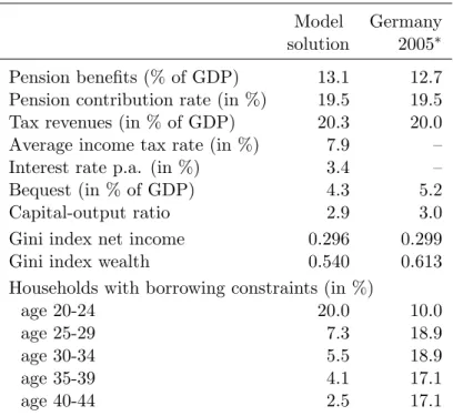
Table 2 reports the calibrated benchmark equilibrium and the respective figures for Ger-many in 2005. The reported bequest in Table 2 are purely accidental since annuity markets are missing. The (endogenous) consumption tax rate is 17 percent which is quite realistic for Germany.
The models income and wealth distribution is more equal than in reality. Partly this reflects the fact that the share of younger cohorts (i.e. those cohorts where income and wealth are less dispersed) in the total population of the model is higher than in Germany. Note that the two lowest productivity classes of the youngest cohort would like to borrow 7The standard pension in Germany is computed for a worker who has received an average wage during employment - i.e. epjR=jR−1 - and amounts to roughly 60 percent of net average earnings.
8In Germany this allowance is currently 3000e for nominal interest income, but 6000eif the source of capital income are dividends.
Table 2: The initial equilibrium
Model Germany
solution 2005∗
Pension benefits (% of GDP) 13.1 12.7
Pension contribution rate (in %) 19.5 19.5
Tax revenues (in % of GDP) 20.3 20.0
Average income tax rate (in %) 7.9 –
Interest rate p.a. (in %) 3.4 –
Bequest (in % of GDP) 4.3 5.2
Capital-output ratio 2.9 3.0
Gini index net income 0.296 0.299
Gini index wealth 0.540 0.613
Households with borrowing constraints (in %)
age 20-24 20.0 10.0
age 25-29 7.3 18.9
age 30-34 5.5 18.9
age 35-39 4.1 17.1
age 40-44 2.5 17.1
*Source: IdW(2007), DIW (2005), SAVE survey.
because they expect a higher productivity (and therefore income) in the future. For older cohorts, the fraction of liquidity constraint agents decreases sharply. After age 35 we hardly observe liquidity constrained households. Recent evidence from the SAVE survey indicates that our model exaggerates borrowing constraints at young ages but understates the constraints in middle-ages.
5
Simulation results
This section presents the quantitative results when we simulate the German Riester reform in four successive steps. In the first simulation we increase the taxation of capital income. Then we introduce traditional IRAs without mandatory annuitization. Next, the IRAs are annuitized after retirement and in the final step we add the special provisions for low-income households. The following subsection explains some technical details of the computation. Then we discuss the macroeconomic and welfare effects of the considered policy reforms.
5.1
Experimental design and welfare computation
Our four reform simulations can be distinguished by alternative combinations ofds, τb,s, ωˆ j
and trj. In the benchmark equilibrium of Table 2 these parameters are set at ds= 1.800
e, τb = ˆs = trj = 0 and ωj = 1. In the first simulation we simply eliminate the saving
allowance (i.e. we set ds = 0).9 Next we combine the increase of ordinary capital income
taxation with the introduction of traditional IRAs, i.e. ds = 0 and ˆs = 2.100 e. Due
to the deferred taxation we assume that inheritances from these accounts are taxed at
τb = 0.165, which equals the average marginal income tax rate in the benchmark. In the
third simulation we add the annuitization of the accounts at the time of retirement, i.e.
ωj = 1 if j < jR and ωj = 0 if j ≥ jR. Finally, we introduce trj >0 in oder to arrive at
the German system.
Of course, all policy reforms affect the tax revenues of the government. In order to balance the intertemporal budget we compute a time-invariant consumption tax rateτc from
τc = B1+ P∞ t=1[GP−Ty,t−Tb,t−Tk,t] (1 +r)1−t ∞ t=1Ct(1 +r)1−t .
The periodical budget is then balanced by the endogenous debt level, i.e.
Bt+1 =Bt(1 +r) +G−Ty,t−τcCt−Tb,t−Tk,t.
Next we turn to the computation of the welfare changes. The welfare criterion which is applied to assess a reform is ex-ante expected utility of an agent, before the productivity level is revealed. For an agent who enters the labor market the expected utility is computed from E[V(z1)] = ·Z E1 ξ(z1)V(z1)1−ηde1 ¸ 1 1−η . (23)
We assume that the reform is implemented after agents know that they have survived but before the productivity shock is revealed. Consequently, the individual welfare effect is derived from the expected utilities in the initial equilibrium and after the reform an-nouncement. Following Auerbach and Kotlikoff (1987, 87) we compute the proportional increase in consumption and leisure (W) which would make an agent in the baseline sce-nario as well off as in the reform scesce-nario. If the expected utility level of an individual age
j in yeartafter the reform isE[V(zj,t)] and the expected utility level on the baseline path
isE[V(zj,0)], the necessary increase (decrease) in percent of initial resources is computed
9Note, however, the saving allowance was not completely eliminated but only severely reduced in Germany during the last years.
from Wj,t = · E[V(zj,t)] E[V(zj,0)] −1 ¸ ×100 (24)
for individuals born before and after the reform. Consequently, a value of Wj,t = 1.0
indicates that this agent would need one percent more resources in the baseline scenario to attain expected utility E[V(zj,t)].
In order to asses the aggregate efficiency consequences, we introduce a Lump-Sum Redis-tribution Authority (LSRA) in the spirit of Auerbach and Kotlikoff (1987, 65f.) as well as Nishiyama and Smetters (2005) and Fehr et al. (2008). The LSRA pays a lump-sum transfer (or levies a lump-sum tax) to each living household in the first period of the transition to bring their expected utility level back to the level of the initial equilibrium. Consequently, age-j agents who were alive in the initial equilibrium are compensated by the transfers vj,1(Wj,1 = 0), that depend on their status in the initial equilibrium and guaranty the initial expected utility levelE[V(zj,0)]. On the other hand, those who enter the labor market in period t of the transition receive a transfer v1,t(W1,t = W∗) which
guaranties them an expected utility level E[V(z1,t)] = V∗. Note that the transfers v1,t
may differ among future cohorts but the expected utility levelV∗ is identical for all. The
value of the latter is chosen by requiring that the present value of all LSRA transfers is zero: J X j=2 Nj Z A×R×P×Ej vj,1(Wj,1 = 0)dX(zj) + ∞ X t=1 v1,t(W1,t =W∗)N1(1 +r)1−t= 0. (25) With V∗ > E[V(z
1,0)] (i.e. W∗ >0), all households in period one who have lived in the previous period would be as well off as before the reform and all current and future new-born households would be strictly better off. Hence, the new policy is Pareto improving after lump-sum redistributions. WithV∗ < E[V(z
1,0)] (i.e. W∗ <0), the policy reform is Pareto inferior after lump-sum redistributions.
5.2
Macroeconomic effects of savings incentives
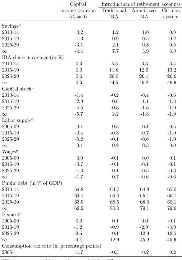
This section discusses the macroeconomic effects of the simulated reforms. The first col-umn (“Capital income taxation”) in Table 3 reports the changes in central macro variables when we extend the taxation of capital income by eliminating the capital allowance.10 The elimination of capital income allowances allows to reduce the consumption tax rate by 1.7 percentage points. Aggregate savings decrease by roughly 4.4 percent in the long-run. Since public debt remains almost constant in the long-run, the capital stock even 10The reform starts in the second period, since we don’t want to alter the taxation of existing assets.
Table 3: Macroeconomic effects of savings taxation and retirement accounts
Capital Introduction of retirement accounts income taxation Traditional Annuitized German
(ds = 0) IRA IRA system
Savingsa
2010-14 0.2 1.2 1.0 0.9
2015-19 -1.3 0.9 0.5 0.2
2025-29 -3.1 2.1 0.8 0.5
∞ -4.4 7.7 3.9 3.9
IRA share in savings (in %)
2010-14 0.0 5.5 6.3 6.4 2015-19 0.0 11.8 12.9 13.2 2025-29 0.0 26.0 26.1 26.6 ∞ 0.0 44.5 46.2 46.9 Capital stocka 2010-14 -1.4 -0.2 -0.4 -0.6 2015-19 -2.9 -0.6 -1.1 -1.3 2025-29 -4.5 -0.3 -1.6 -1.9 ∞ -5.7 2.2 -1.8 -1.9 Labor supplya 2005-09 -0.1 0.3 -0.1 -0.5 2015-19 -0.4 -0.3 -0.7 -1.0 2025-29 -0.2 -0.1 -0.6 -1.0 ∞ -0.1 -0.2 0.3 0.0 Wagesa 2005-09 0.0 -0.1 0.0 0.1 2015-19 -0.7 -0.1 -0.1 -0.1 2025-29 -1.3 -0.1 -0.3 -0.3 ∞ -1.7 0.7 -0.6 -0.6
Public debt (in % of GDP)
2010-14 64.8 64.7 64.8 65.0 2015-19 64.1 65.0 65.1 65.1 2025-29 63.0 68.5 68.0 68.1 ∞ 62.2 80.0 79.1 79.6 Bequesta 2005-09 0.0 0.1 0.0 -0.1 2015-19 -1.2 -0.9 -2.9 -3.0 2025-29 -2.5 -0.1 -12.3 -12.5 ∞ -4.1 12.9 -45.2 -45.6
Consumption tax rate (in percentage points)
2005- -1.7 -0.3 -0.2 0.2
decreases by 5.7 percent, so that the interest rate increases by about 0.3 percentage points. The lower capital stock reduces wages and labor supply. Finally, due to lower savings also accidental bequest decrease by about 4 percent in the long-run.
In the following two simulations, we keep the full taxation of ordinary asset returns but introduce retirement accounts without (“Traditional IRA”) and with (“Annuitized IRA”) mandatory annuitization of benefits after retirement. Younger and future generations now increase savings in tax-favored accounts so that aggregate savings rise throughout the transition. Since tax revenues decline and are shifted from current to future periods, the consumption tax rate is higher than in the first simulation and public debt increases during the transition. Due to higher public debt, the capital stock and wages only increase slightly in the long-run without annuitization. Note that we would get quite similar effects for savings and the capital stock as ˙Imrohoro˘glu et al. (1998) if we would not alter capital income taxation. From the figures in Table 3 we can also compute that in the long-run about 16 percent of IRA contributions represent new savings. 11 This corresponds quite well with Attanasio and DeLeire (2002) who found that in the United Kingdom about 9 percent of IRA contributions are from new savings.
However, matters are quite different when we introduce annuitized accounts in the next simulation. Assets of deceased are now transferred to surviving elderly. Consequently, while bequests still increase in the second simulation, they decrease now dramatically so that long-run savings and the capital stock are much lower than before. In the last column (“German system”) we keep annuitization but introduce the direct savings subsidies. Of course, such a program increases cost, therefore the consumption tax has to rise while savings and the capital stock change as before. In the German system, those people who contribute less than 4 percent of their income can increase the transfer rate for given savings if they work less, see the definition (3). Consequently, this feature of the saving subsidy design induces a negative labor supply effect which is evident in Table 3.
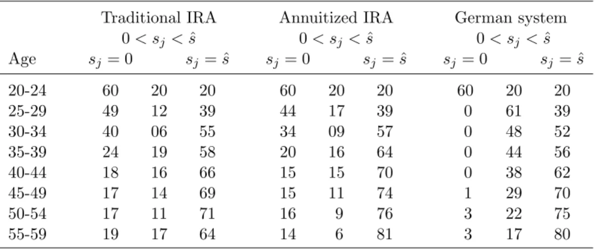
Whereas Table 3 documents that the share of savings in retirement accounts rises dur-ing the transition, Table 4 reports how cohorts contribute to the accounts in the new long-run equilibrium. People first have to build up precautionary savings against income uncertainty. Consequently, 60 percent of the youngest cohort do not contribute to the accounts at all. With rising age participation rates and contributions increase since ex-isting precautionary savings reduce the exposure to income uncertainty.12 Note that with annuitized accounts contributions rise especially before retirement. Since after retirement
11This figure is derived from 1
0.445(1−1.0771 ) = 0.161.
12This corresponds to the findings of Hrung (2002) who shows that in the U.S. IRA savings are lower for individuals exposed to high income risk.
income uncertainty is eliminated, precautionary savings are reshuffled to retirement ac-counts in order to increase longevity insurance. B¨orsch-Supan et al. (2007, 18) confirm for Germany that participation increases with age initially but then it declines again after age 50. Currently Riester pensions are most common in the 30 to 49 age group. One reason for the low participation rate among elderly might be that our model does not reflect the transitional period between 2002 and 2008 where subsidy payments were much lower and the regulation of Riester pensions was more complicated. In addition, we also do not consider the future reduction of public pension benefits. The latter induces a clear incentive especially for middle-age and young individuals to save more for retirement.
Table 4: Average participation in retirement accounts (in %)
Traditional IRA Annuitized IRA German system
0< sj <ˆs 0< sj <sˆ 0< sj <sˆ Age sj = 0 sj = ˆs sj = 0 sj = ˆs sj = 0 sj = ˆs 20-24 60 20 20 60 20 20 60 20 20 25-29 49 12 39 44 17 39 0 61 39 30-34 40 06 55 34 09 57 0 48 52 35-39 24 19 58 20 16 64 0 44 56 40-44 18 16 66 15 15 70 0 38 62 45-49 17 14 69 15 11 74 1 29 70 50-54 17 11 71 16 9 76 3 22 75 55-59 19 17 64 14 6 81 3 17 80
Apart from the initial cohorts, the German system in the right part of Table 4 induces an extremely high participation rate. Of course, this mainly reflects changes in the behavior of low-income households. Table 5 compares the participation rate of the bottom decile in the traditional retirement account with annuitization and in the German system. Whereas with traditional accounts still 56 percent of the bottom decile don’t contribute at all in the period before retirement, this fraction decreases to 13 percent in the German system. Consequently, the direct subsidy payments are quite effective in increasing participation and contributions among low-income households. This is also confirmed by B¨orsch-Supan et al. (2007, 19) who document that Riester accounts are particularly popular among larger families with children.
5.3
Welfare effects of saving incentives
Next we turn to welfare consequences for different cohorts in the reform year and the long-run without and with compensation payments from the LSRA. As already explained
Table 5: Participation of low-income households (in %)
Annuitized IRA German system
0< sj <ˆs 0< sj <sˆ Age sj = 0 sj = ˆs sj = 0 sj = ˆs 20-24 100 0 0 100 0 0 25-29 100 0 0 0 100 0 30-34 99 1 0 0 100 0 35-39 90 8 2 0 100 0 40-44 74 23 3 0 98 2 45-49 72 18 10 1 92 7 50-54 65 18 17 5 79 16 55-59 56 20 24 13 64 23
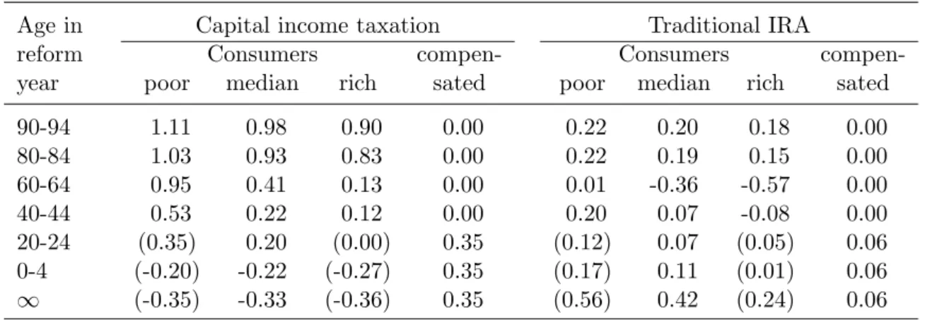
above, we first compute the welfare changes of agents before their productivity is revealed and then derive an average welfare change for the different productivity types in each cohort that already lives in the initial equilibrium. Therefore, Table 6 distinguishes in each cohort between “poor”,“median”, and “rich” households. “Poor” agents are the 10 percent of the cohort with the lowest realized productivity level, “median” are those 20 percent who realize a medium productivity level and “rich” are those 20 percent of the cohort with the highest productivity.13 For newborn cohorts along the transition path we are not able to disaggregate ex-ante welfare effects. Consequently, we report in the middle column the ex-ante welfare change of the whole cohort and in brackets the (ex-post) welfare changes for “poor” and “rich” newborn households after their productivity is revealed to them. Table 6 compares the extension of capital income taxation and the introduction of (non-annuitized) traditional retirement accounts in the present model. Not surprisingly, an increase in capital income taxation balanced by reduced consumption taxes is especially beneficial for medium and old-aged households with low wealth holdings. All households gain from the reduction of consumption taxation, but poor elderly are also hardly affected by the increase in capital income taxation. While medium-aged households have build-up assets already, they are hurt by the increase of capital income taxation. Since the reform reduces wages in the long-run significantly, generations born in the future lose. The differences within the cohorts are rather insignificant. Next we simulate the reform with lump-sum compensation payments of the LSRA in order to isolate the aggregate efficiency consequences of the rise in capital income taxation.14 The
13For pensioners we aggregate the respective fractions in earning points.
compensated welfare changes for all generations alive in the initial equilibrium are then zero and newborn generations experience identical relative consumption increases. As shown in the forth column, rising capital income taxes increase aggregate efficiency by 0.35 percent of remaining resources. This is due to the fact that the reformed tax system (with more income and less consumption taxation) offers more income insurance.15
Table 6: Welfare effects of alternative capital income tax regimes
Age in Capital income taxation Traditional IRA
reform Consumers compen- Consumers
compen-year poor median rich sated poor median rich sated
90-94 1.11 0.98 0.90 0.00 0.22 0.20 0.18 0.00 80-84 1.03 0.93 0.83 0.00 0.22 0.19 0.15 0.00 60-64 0.95 0.41 0.13 0.00 0.01 -0.36 -0.57 0.00 40-44 0.53 0.22 0.12 0.00 0.20 0.07 -0.08 0.00 20-24 (0.35) 0.20 (0.00) 0.35 (0.12) 0.07 (0.05) 0.06 0-4 (-0.20) -0.22 (-0.27) 0.35 (0.17) 0.11 (0.01) 0.06 ∞ (-0.35) -0.33 (-0.36) 0.35 (0.56) 0.42 (0.24) 0.06
aChange are reported in percentage of initial resources.
The introduction of (non-annuitized) traditional retirement accounts in the right part of Table 6 neutralizes (at least partly) the increase in capital income taxation. Since consumption taxes fall much less, the welfare gains of already retired generations are now much lower than in the first simulation. Medium-income and rich households who retire in the reform year even experience significant welfare losses. They can’t benefit from the new accounts, consequently they fully bear the increase of capital income taxes but now they benefit from reduced consumption taxes much less. Welfare of newborn and future generations now increases after the reform since these cohorts can reduce their capital income tax burden significantly by saving in the accounts and long-run wages increase now slightly. Since higher wages relax existing liquidity constraints, long-run poor households are significantly better off than the respective rich ones. Since now the consumption tax rate remains almost constant, the reform only changes the taxation of different saving motives. Although highly elastic old-age savings are exempt from taxation, the aggregate efficiency gains are fairly small.
The left part of Table 7 shows that annuitization mainly reduces the welfare of newborn are available on request.
15This corresponds with the results of Nishiyama and Smetters (2005) who find in a similar set-up an aggregate efficiency loss after a switch from income to consumption taxation.
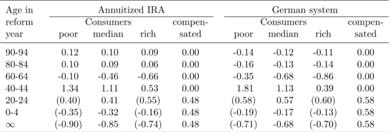
and future generations. Already retired cohorts are only affected by the slightly higher consumption tax rate. Since former intergenerational transfers are substituted by transfers within a generation, working generations in the reform year are significantly better off than before. They still receive bequest from the elderly and benefit from increased longevity insurance. On the other hand, future generations are much worse off than before since they are hurt by the significant reduction of unintended bequest. In the long-run the welfare reduction amounts to 0.85 percent of remaining resources. Note that future generations lose although aggregate efficiency rises significantly by roughly 0.5 percent of aggregate resources. The latter reflects the value of the longevity insurance which is provided by the annuity.
Table 7: Welfare effects of annuitized retirement accounts
Age in Annuitized IRA German system
reform Consumers compen- Consumers
compen-year poor median rich sated poor median rich sated
90-94 0.12 0.10 0.09 0.00 -0.14 -0.12 -0.11 0.00 80-84 0.10 0.09 0.06 0.00 -0.16 -0.13 -0.14 0.00 60-64 -0.10 -0.46 -0.66 0.00 -0.35 -0.68 -0.86 0.00 40-44 1.34 1.11 0.53 0.00 1.81 1.13 0.39 0.00 20-24 (0.40) 0.41 (0.55) 0.48 (0.58) 0.57 (0.60) 0.58 0-4 (-0.35) -0.32 (-0.16) 0.48 (-0.19) -0.17 (-0.13) 0.58 ∞ (-0.90) -0.85 (-0.74) 0.48 (-0.71) -0.68 (-0.70) 0.58
aChange are reported in percentage of initial resources.
Finally, in the right part of Table 7 the German system of (optional) direct subsidies reduces welfare of retired households due to the increase in consumption taxes. As one would expect, low-income newborn and future households are better off compared to the previous simulation, but they still experience welfare losses from the reform. Of course, they benefit directly from the subsidies but they are also hurt by the higher consumption taxes. On the other hand, future rich households are almost not affected. Direct subsidies for low-income households improve the insurance properties of the tax system while they also distort labor supply. Since the insurance effect dominates the distortionary effect, the last column reports only a slight increase in aggregate economic efficiency compared to the previous simulation.
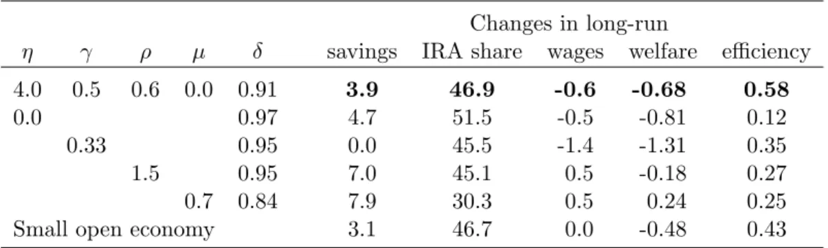
Table 8: Sensitivity analysis for the German system
Changes in long-run
η γ ρ µ δ savings IRA share wages welfare efficiency
4.0 0.5 0.6 0.0 0.91 3.9 46.9 -0.6 -0.68 0.58
0.0 0.97 4.7 51.5 -0.5 -0.81 0.12
0.33 0.95 0.0 45.5 -1.4 -1.31 0.35
1.5 0.95 7.0 45.1 0.5 -0.18 0.27
0.7 0.84 7.9 30.3 0.5 0.24 0.25
Small open economy 3.1 46.7 0.0 -0.48 0.43
5.4
Sensitivity analysis
The positive efficiency effects and the negative long-run welfare effects of the German system turn out to be quite robust. Table 8 reports the long-run macroeconomic and welfare effects as well as efficiency consequences for alternative parameter combinations and economic assumptions. For better comparison the first line repeats (in bold numbers) the results for the benchmark case from Tables 3 and 7. With risk neutral agents (i.e. when η = 0.0) precautionary savings decrease so that the time preference rate has to increase in order to recalibrate the initial equilibrium with the same capital-output ratio as in Table 2. Risk neutral individuals react stronger to the tax incentives. Consequently, aggregate savings increase stronger and the long-run IRA share is higher than in the benchmark. Therefore, unintended bequest fall much stronger so that long-run welfare is even lower than in the benchmark. Since risk neutral individuals don’t value the insurance provision of the annuitized accounts, the efficiency gain is reduced from 0.6 to 0.1 percent of aggregate resources. Note that this is very close to the aggregate efficiency gain in the traditional IRA system of Table 6. In both cases aggregate efficiency changes are mainly due to the separate taxation of different savings motives.
Next we reduce the intertemporal elasticity of substitution from 0.5 to 0.33. Since the consumption profile becomes flatter, initial savings fall and the time preference rate has to increase again to stabilize the capital-output ratio. Now savings incentives work much less than in the benchmark. Savings in retirement accounts mainly represent funds which are shifted from already existing accounts. As a consequence, aggregate savings remain constant in the long-run. Since public debt increases as before, the capital stock decreases much stronger and wages fall by 1.4 percent. The latter hurts future generations so that long-run welfare decreases more than in the benchmark. Aggregate efficiency increases slightly less than in the benchmark since intertemporal distortions are reduced less when the intertemporal elasticity of substitution is low.
In the following simulation we assume an extremely high (compensated) labor supply elasticity of about 1 by setting ρ= 1.5. In this case households work and save less in the initial equilibrium so that again the time preference rate has to increase. The reaction of labor supply is now much stronger than in the benchmark simulation. Employment even falls in the long-run by 0.7 percent. At the same time aggregate savings rise much stronger so that long-run wages now even increase by about 0.5 percent. Higher wages and higher bequest reduce the long-run welfare losses compared to the benchmark. Since the reform increases distortions of labor supply, aggregate efficiency decreases with a higher intratemporal elasticity of substitution.
Up to now people had no bequest motive. When we introduce such a “joy of bequest giving” motive, savings rise so that the time preference rate has to decrease significantly in order to recalibrate the initial equilibrium. A bequest motive has two major consequences. First, annuitized accounts are less attractive. Second, additional resources of the surviving elderly (from annuitized accounts) are now not consumed but saved for the descendants. As a consequence, aggregate savings increase quite strongly while at the same time the IRA share remains much low. Therefore, the capital stock increases much stronger so that wages rise and future generations even experience a welfare gain. Of course, since now people take less advantage of the insurance properties of accounts, aggregate efficiency decreases compared to the benchmark.
Finally, in the small open economy we can keep all parameters from the benchmark but keep factor prices constant. People save now slightly less compared to the benchmark and long-run generations lose slightly less due to constant wages. The aggregate efficiency gain is smaller compared to the benchmark probably because of the dampened savings reaction.
6
Discussion
This study intends to evaluate the macroeconomic and welfare consequences of the intro-duction of tax-favored “Riester pensions” in Germany. Since savings in the accounts are tax deferred, we assume that the government balances the intertemporal budget by the consumption tax so that public debt increases during the transition. We find a long-run decrease in the capital stock and wages of about 2 and 0.6 percent, respectively, although aggregate savings increase during the transition. The reform increases economic efficiency by roughly 0.6 percent of aggregate resources but reduces the welfare of future generations almost in the same relative amount. The efficiency gain is mostly due to the fact that the reform improves the insurance properties of the tax system and allows to tax different savings motives separately. Long-run welfare decreases because accidental bequest fall
dramatically when retirement accounts include provisions for mandatory annuitization. Finally, the study indicates that the special provisions for low-income households are suc-cessful in increasing the participation of this group. However, the particular design of the German system has a negative side effect on labor supply.
Therefore, the present study highlights the importance of including transitional dynamics in tax and pension reform analysis. Since the long-run welfare changes are mainly due to intergenerational redistribution, they don’t even indicate the direction of the overall efficiency effects. Our results confirm the back-of-the-envelop calculations in Fehr and Habermann (2008) who quantify efficiency efficiency effects of the introduction of annuities in a stylized model.
Of course, the simulated reforms could be extended in various directions. It is no problem to fully annuitize retirement account savings even before retirement, allow (as in Germany) to withdraw a lump-sum amount at time of retirement, or model a choice between an immediate annuitization at the beginning of retirement and a fixed pay-out plan combined with delayed annuitization. However, these extensions have only very minor effects on aggregate efficiency. Fehr, et al. (2008) also consider alternative financing scenarios, contribution ceilings and direct subsidy payments. While each reform design alters the intergenerational welfare consequences, the aggregate efficiency effect is hardly changed. Of course, it would be no problem to include additional elements of the German Riester reform such as the reduction of the unfunded public pension system. This extension would increase the incentives to contribute to the accounts but it would complicate the welfare analysis of Riester accounts. For this reason this extension is left to future research.
Appendix A: Computational method
In order to compute a solution we have to discretize the state space. The state of a household is determined by zj = (j,aj,aRj, epj, ej) ∈ J ×A ×R × P × Ej where
J = {1, . . . , J}, A = {a1, . . . ,anA}, R = {aR,1, . . . ,aR,nR}, P = {ep1, . . . , epnP} and
Ej ={e1j, . . . , enjE} are discrete sets. In this paper we use J = 16, nA =nR = 12, nP = 5
and nE = 6. The initial values for efficiencies are: ξ(1,0,0,0, e11) = ξ(1,0,0,0, e21) = 0.1 and ξ(1,0,0,0, e3
1) = · · ·=ξ(1,0,0,0, e61) = 0.2.
For all these possible states zj we compute the optimal decision of households from (5).
The pension grid is equidistant while the asset grid has increasing intervals between two grid points. This is useful since the value function is heavily curved for low values of assets. Sinceu(cj, `j) is not differentiable in every (cj, `j) andV(zj+1) is only known in a discrete set of pointszj+1 ∈ {j+ 1} ×A×R×P×Ej, this maximization problem can not
be solved analytically. Therefore we have to use the following numerical maximization and interpolation algorithms to compute households optimal decision:
1. Compute (5) in ageJfor all possiblezJ. Notice thatV(zJ+1) = 0 and households are not allowed to work anymore. Hence, in the optimum households should consume everything they have.
2. For j =J−1, . . . ,1:
Find (5) for all possible zj by using Powell’s algorithm (Press et. al., 2001, 406ff.).
Since this algorithm requires a continuous function, we have to interpolateV(zj+1).
Having computed the dataV(zj+1) for allzj+1 ∈ {j+1}×A×R×P×Ej in the last
step, we can now find a function spj+1 which satisfies the interpolation conditions
spj+1(j+ 1,akj+1,ajR,l+1, epmj+1) = EV(zj+1) (26)
for all k = 1, . . . , nA, l = 1, . . . , nR and m = 1, . . . , nP. In this paper we use
multidimensional cubic spline interpolation, i.e. spj : S3× S3× S3 → R, whereas
S3 is the space of all one-dimensional, twice continuously differentiable, piecewise third-order polynomial functions and S3× S3× S3 is its tensor product (cf. Judd (1998, 225ff.)). For further information see Habermann and Kindermann (2007).
Appendix B: Markov transition matrices
Age dependent Markov transition matrices
Age 20-24 Age 25-29
Future productivity level Future productivity level
1 2 3 4 5 6 1 2 3 4 5 6 1 0.30 0.16 0.27 0.07 0.06 0.13 0.31 0.17 0.22 0.08 0.10 0.11 2 0.15 0.18 0.19 0.24 0.12 0.13 0.15 0.22 0.28 0.13 0.10 0.11 Current 3 0.07 0.18 0.39 0.17 0.12 0.08 0.08 0.11 0.33 0.25 0.14 0.09 productivity 4 0.09 0.07 0.15 0.33 0.22 0.15 0.08 0.08 0.21 0.31 0.22 0.09 level 5 0.07 0.05 0.13 0.24 0.34 0.17 0.05 0.05 0.12 0.21 0.32 0.24 6 0.05 0.04 0.10 0.12 0.23 0.46 0.06 0.06 0.09 0.12 0.22 0.46 Age 30-34 Age 35-39
Future productivity level Future productivity level
1 2 3 4 5 6 1 2 3 4 5 6 1 0.33 0.22 0.21 0.09 0.09 0.07 0.37 0.20 0.22 0.13 0.05 0.05 2 0.18 0.25 0.30 0.14 0.05 0.07 0.22 0.29 0.32 0.12 0.03 0.02 Current 3 0.09 0.15 0.35 0.24 0.11 0.06 0.12 0.16 0.38 0.20 0.09 0.05 productivity 4 0.07 0.06 0.24 0.33 0.21 0.09 0.04 0.04 0.24 0.40 0.22 0.07 level 5 0.05 0.02 0.11 0.24 0.38 0.20 0.02 0.04 0.07 0.21 0.44 0.22 6 0.03 0.04 0.05 0.08 0.23 0.58 0.02 0.02 0.04 0.07 0.22 0.63 Age 40-44 Age 45-49
Future productivity level Future productivity level
1 2 3 4 5 6 1 2 3 4 5 6 1 0.49 0.24 0.15 0.04 0.06 0.02 0.45 0.26 0.22 0.04 0.01 0.01 2 0.17 0.31 0.36 0.09 0.05 0.03 0.15 0.32 0.33 0.14 0.03 0.03 Current 3 0.07 0.13 0.40 0.25 0.10 0.05 0.08 0.11 0.44 0.27 0.07 0.02 productivity 4 0.06 0.06 0.20 0.40 0.21 0.08 0.05 0.04 0.16 0.40 0.29 0.06 level 5 0.02 0.02 0.09 0.21 0.47 0.18 0.04 0.02 0.08 0.19 0.46 0.20 6 0.02 0.02 0.05 0.07 0.16 0.66 0.02 0.03 0.05 0.04 0.15 0.70 Age 50-54
Future productivity level
1 2 3 4 5 6 1 0.42 0.22 0.21 0.07 0.04 0.04 2 0.14 0.30 0.35 0.11 0.06 0.04 Current 3 0.11 0.12 0.37 0.25 0.11 0.03 productivity 4 0.04 0.05 0.19 0.41 0.24 0.07 level 5 0.04 0.03 0.09 0.20 0.45 0.19 6 0.03 0.05 0.07 0.05 0.15 0.66
References
Attanasio, O.P. and T. DeLeire (2002): The effect of individual retirement accounts on household consumption and national saving,Economic Journal 112, 504-538. Auerbach, A.J. and L.J. Kotlikoff (1987): Dynamic fiscal policy, Cambridge University
Press, Cambridge.
Benjamin, D.J. (2003): Does 401 (k) eligibility increase savings? Evidence from propen-sity score subclassification,Journal of Public Economics 87 (5-6), 1259-1290. Bernheim, D. (2002): Taxation and saving, in: A. Auerbach und M. Feldstein (Hrsg.),
Handbook of Public Economics, Vol. 3, Amsterdam, 1173-1250.
B¨orsch-Supan, A., A. Reil-Held and D. Schunk (2007): The savings behavior of German households: First experiences with state promoted private pensions, Working paper 136-2007, MEA Mannheim.
Bomsdorf, E. (2003): Sterbewahrscheinlichkeiten der Periodensterbetafeln f¨ur die Jahre 2000 bis 2100, Eul Verlag, K¨oln.
Cagetti, M. (2001): Interest elasticity in a life-cycle model with precautionary savings,
American Economic Review 91(2), 418-421.
De Nardi, M. (2004): Wealth inequalities and intergenerational links, Review of Eco-nomic Studies71, 743-768.
Deutsches Institut f¨ur Wirtschaftsforschung (DIW) (2005): Verteilung von Verm¨ogen und Einkommen in Deutschland, Wochenbericht des DIW Berlin Nr. 11, 199-207. Epstein, L.G. and S.E. Zin (1991): Substitution, risk aversion, and the temporal
behav-ior of consumption and asset returns: An empirical analysis, Journal of Political Economy 99, 263-286.
Fehr, H. (1999): Welfare effects of dynamic tax reforms, Mohr Siebeck, Tuebingen. Fehr, H. and C. Habermann (2008): Welfare effects of life annuities: Some clarifications,
Economics Letters (forthcoming).
Fehr, H., C. Habermann and F. Kindermann (2008): Tax-favored retirement accounts: Are they efficient in increasing savings and growth? Working Paper, Universit¨at W¨urzburg.
Fehr, H. and Ø. Thøgersen (2008): Social security and future generations, in: R. Brent (ed.), Handbook on research in cost-benefit analysis, Edward Elgar (forthcoming). Feldstein, M. (1997): The costs and benefits of going from low inflation to price stability,
in: C. Romer and D. Romer (eds.),Reducing inflation, University of Chicago Press, Chicago and London, 123-156.
Fuster, L., A. ˙Imrohoro˘glu and S. ˙Imrohoro˘glu (2005): Personal security accounts and mandatory annuitization in a dynastic framework, CESifo Working Paper No. 1405, Munich.
Habermann, C. and F. Kindermann (2007): Multidimensional spline interpolation: The-ory and applications,Computational Economics 30(2), 153-169.
Hrung, W.B. (2002): Income uncertainty and IRAs, International Tax and Public Fi-nance 9(5), 591-599.
˙Imrohoro˘glu, A., S. ˙Imrohoro˘glu and D.H. Joines (1998): The effect of tax-favored retire-ment accounts on capital accumulation,American Economic Review 88 (4), S.749-768.
Institut der deutschen Wirtschaft (IdW) (2007): Deutschland in Zahlen, K¨oln. Judd, K.L. (1998): Numerical Methods in Economics, The MIT Press, Cambridge. Krueger, D. (2006): Public insurance against idiosyncratic and aggregate risk: The case
of social security and progressive income taxation, CESifo Economic Studies 52, 587-620.
Nishiyama, S. and K. Smetters (2005): Consumption taxes and economic efficiency with idiosyncratic wage shocks,Journal of Political Economy 113, 1088-1115.
OECD (2004), Tax-favoured Retirement Saving, OECD Economic Studies No. 39, Paris. Pecchenino, R.A. and P.S. Pollard (1997): The effects of annuities, bequest, and aging in an overlapping generations model of endogenous growth,Economic Journal 107, 26-46.
Press, W.H. , S.A. Teukolsky, W.T. Vetterling and B.P. Flannery (2001): Numerical Recipes in Fortran 77, Volume 1 of Fortran Numerical Recipes, Cambridge Univer-sity Press, Cambridge.