Average Marginal Income Tax
Rates in New Zealand, 1907-2009
Debasis Bandyopadhyay, Robert Barro,
Jeremy Couchman, Norman Gemmell,
Gordon Liao and Fiona McAlister
WORKING PAPER 01/2012
July 2012
The Working Papers in Public Finance series is published by the Victoria
Business School to disseminate initial research on public finance topics, from
economists, accountants, finance, law and tax specialists, to a wider audience. Any
opinions and views expressed in these papers are those of the author(s). They should
not be attributed to Victoria University of Wellington or the sponsors of the Chair in
Public Finance.
Further enquiries to:
The Administrator
Chair in Public Finance
Victoria University of Wellington
PO Box 600
Wellington 6041
New Zealand
Phone: +64-4-463-9656
Emil:
cpf-info@vuw.ac.nz
Papers in the series can be downloaded from the following website:
Average Marginal Income Tax
Rates in New Zealand, 1907-2009
D e b a s i s B a n d y o p a d h y a y , R o b e r t B a r r o ,
J e r e m y C o u c h m a n , N o r m a n G e m m e l l ,
G o r d o n L i a o a n d F i o n a M c A l i s t e r
A b s t r a c t
Estimates of marginal tax rates (MTRs) faced by individual economic agents,
and for various aggregates of taxpayers, are important for economists testing
behavioural responses to changes in those tax rates. This paper reports
estimates of a number of personal marginal income tax rate measures for New
Zealand since 1907, focusing mainly on the aggregate income-weighted
average MTRs proposed by Barro and Sahasakul (1983, 1986) and Barro and
Redlick (2011). The paper describes the methodology used to derive the
various MTRs from original data on incomes and taxes from Statistics
New
Zealand Official Yearbooks
(NZOYB), and discusses the resulting estimates.
J E L C L A S S I F I C A T I O N
H20; H24
T a b l e o f C o n t e n t s
Abstract ... i
Table of Contents ... ii
List of Tables... iii
List of Figures ... iii
1 Introduction ... 4
2 Personal Income Taxation ... 5
2.1 Sources of Government Revenue ... 5
2.2 Tax Rate Definitions ... 7
2.3 The New Zealand Personal Income Tax ... 8
3 New Zealand Income Distribution Data ... 11
3.1 Income Data ...12
3.2 Exemptions Data ...13
3.3 Non-Filer Incomes ...13
4 Calculating AMTRs – Methodology ... 14
4.1 Applying the Barro-Sahasakul Approach ...14
4.2 Examples of AMTR calculations ...15
5 Income-weighted AMTRs: 1907-2009 ... 17
5.1 The Overall pattern of AMTRs ...17
5.2 Relationships between Exemptions, Non-Filed Incomes and AMTRs ...20
5.3 Decomposing Changes in the AMTRs...21
5.4 Earned vs. Unearned Income ...25
5.5 The Effect of Family Tax Credits, Benefits and ACC ...26
5.6 Reliability of AMTR Estimates ...27
6 Conclusions ... 28
References ... 29
Data Sources ... 30
Appendix 1: The NZ ‘Multi-Slope’ Income Tax System 1914-1939 ... 31
A1.1 The 1914 tax structure ...31
A1.2 The 1917 ‘war-time’ tax structure ...32
Appendix 2: Income Distribution Data ... 34
Appendix 3: Exemptions Data ... 36
L i s t o f T a b l e s
Table 1 – Income tax rates, 1910-1912 ... 9
Table 2 – The AMTR calculations, 1980 ... 15
Table 3 – Average marginal tax rates (in percent), 1907-2009... 19
Table 4 – Correlation matrix of AMTR changes... 24
Table 5 – EMTRjs for family tax credits, welfare benefits and ACC ... 26
Table A1 – Abatement of general exemption, 1917-1935 ... 37
Table A2 – Exemptions by size of income for the 1925/26 income year ... 37
Table A3 – Estimated average income of non-filers from 1926 census data ... 39
Table A4 – Estimated non-filer income ... 39
L i s t o f F i g u r e s
Figure 1 – Government tax revenue by source, 1903 – 2011 ... 6
Figure 2 – Top effective marginal tax rates for New Zealand, 1907-2009* ... 11
Figure 3 – Distribution of total and earned assessable income, 1925 ... 13
Figure 4 – Income distribution and tax structure, 1950 ... 16
Figure 5 – AMTRs for New Zealand 1907-2009 ... 18
Figure 6 – Proportions of taxed, exempt and non-filed income, 1907 – 1983 ... 21
Figure 7 – AMTRs and tax exempt/non-filed income, 1922-1983 ... 23
Figure 8 – Cross-plot of AMTR and non-zero EMTR
javerage, 1922-1983 ... 23
Figure 9 – Changes in unweighted averages of EMTR
js and AMTRs,
1922-1983 25
Figure 10 – AMTRs for earned and unearned income, 1922-1956 ... 26
Figure A1 – Marginal and average tax rates in the 1914 tax structure ... 32
Figure A2 – Marginal and average tax rates in the 1917 tax structure ... 33
Figure A4 – Decomposition of total personal income into filers/non-filers,
1907-1958 ... 40
1
I n t r o d u c t i o n
A focus on marginal tax rates (MTRs) is ubiquitous among studies of the numerous economic outcomes that can be impacted by taxation. The ‘outcomes’ of interest are often at the individual taxpayer level; e.g. labour supply choices, personal taxable incomes, consumption-savings choices, individual welfare costs. The aggregation of these micro-level behaviours in response to MTRs into macro-level outcomes has become an important focus of research in recent years. It now includes an extensive literature on the impacts of taxation (and public expenditure, deficits, etc) on aggregate GDP, national savings, investment, and other macro-level outcomes.
The recent global recession in particular has prompted macroeconomists to reconsider the effectiveness or otherwise of fiscal stimulus packages on GDP and other macro variables, with analysis and evidence on this issue dominating recent debate in the US over the merits of tax cuts and stimulus spending. Similarly, for New Zealand, recent tax and spending reforms, including changes to key MTRs have implications for net fiscal injections and future fiscal deficits. In addition, the literature testing the impacts of fiscal policy on longer-run economic growth has increasingly investigated the importance of MTRs faced by different agents and
types of economic activity, and the impact of exogenous changes in public expenditures.1
Among the difficulties confronting those macro-level studies are problems measuring the ‘true’ marginal tax rates of interest. Lack of suitable data has often meant that ‘implicit’ average tax
rates are used, obtained using tax revenue data. As a consequence, the endogenous
relationships among ‘true’ marginal tax rates, tax bases and GDP, which together determine tax revenues, become difficult to disentangle. Recently Barro and Redlick (2011) have proposed ways to help overcome these endogeneity concerns. Firstly, they estimate multiplier effects on US GDP over a long period (1917-2006) and consider both taxes and public spending
simultaneously. For the latter they use public defence expenditures and expected defence
expenditures (“defence news”) to help overcome spending endogeneity. This requires a number of war episodes to assist with identification. Secondly, on the tax side, following methods developed by Barro and Sahasakul (1983, 1986), they argue that an economy-wide ‘average marginal tax rate’ (AMTR) using taxpayer income shares as weights provides a suitable marginal tax rate measure to capture the potential aggregate responses of GDP to changes in individual personal tax incentives.
The present paper reports estimates of a number of MTR measures for New Zealand, focusing especially on the Barro and Sahasakul AMTRs for personal income taxes. The estimates cover around a century of New Zealand’s personal income tax regime, from 1907 to the present. The paper contributes to the literature in three main areas. First, we provide a comprehensive time-series database of various marginal income tax rate variables over more than 100 years. We calculate effective marginal income tax rates by adjusting for various additional taxes (social security, war taxes etc.) and exemptions. The inclusion of the impact of social welfare benefits was beyond the scope of our analysis; however, we have provided a point estimate for 2008. Secondly, we extend the limited database on incomes (available from Inland Revenue from 1981) to include aggregate level income data by income class from 1907 assembled from Statistical Yearbooks and other primary sources. Thirdly, we propose a methodology to construct a Barro-Sahasakul type measure of AMTRs using the data available for New Zealand.
1 Recent contributions include Lee and Gordon (2005), and Angelopoulos et al. (2007), Romero-Avila and Strauch (2008), Romer and
This dataset has the potential to form a useful basis from which to answer a number of empirical questions relating to the output and other effects of fiscal policy in New Zealand. The paper is organised as follows. Section 2 discusses New Zealand’s personal income tax system, putting it in historical perspective. Sub-section 2.1 begins by putting the income tax in the context of New Zealand’s overall revenue-raising regime of which income taxation was initially only a small part. Secondly, since a number of tax rate definitions are used throughout the paper, sub-section 2.2 introduces those definitions, including the Barro-Sahasakul AMTR measure. In view of the important role of income-weighting in the AMTR measure, section 3 introduces the available income data and its distribution across income classes over the period. Section 4 then describes the methodology used to construct the AMTR series for New Zealand, and section 5 presents and discusses the AMTR results.
2
P e r s o n a l I n c o m e T a x a t i o n
This section first shows how income taxation has evolved within the New Zealand tax system since the beginning of the twentieth century, introduces a number of marginal tax rate definitions used later in the paper, and discusses some key historical aspects of the New Zealand income tax system that affect calculations of the various MTR measures.
2 . 1
S o u r c e s o f Go v e r n me n t R e v e n u e
Over the course of New Zealand’s fiscal history the sources of government revenue have changed as the economy has developed and the role of government increased. While taxation is only one source of government revenue, it is the most important, though the proportions of expenditure financed by taxes, charges for services and borrowing have varied considerably over the years.
The composition of tax revenue has changed significantly over the last century. In the early colonial period it was based heavily on customs and excise duties; these accounted for more than 90 percent of tax revenue in 1875-76, with the balance being provided by stamp duties.
Excise duties were charged on commodities such as alcohol, tobacco and sugar.2 At that stage
in New Zealand’s history customs duty acted similarly to a general sales tax on commodities since a very high proportion of commodities was imported.
In the last years of the nineteenth century taxation was extended into two new areas: an excise on beer, and taxes on land and property. Customs and excise duties remained the predominant source of revenue, but from 1891 income was introduced as a new tax base in the Land and Income Tax Act. Nevertheless, during the early part of the twentieth century the government continued to rely on customs and excise duties for revenue, and it was not until the on-set of the First World War (WWI) that income taxes began to contribute a substantial share of total revenues.
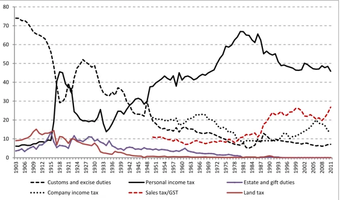
These trends can be seen in Figure 1 which shows the changing composition of the tax revenue
base from 1903 to 2011.3 Taxes are split into customs and excise duties, personal income tax,
2 See Goldsmith (2008) for data on tax revenue shares during the nineteenth century from 1840.
3 The figure uses data from several different sources. From 1903 to 1949 data is taken from New Zealand Official Yearbooks. These did not
include categories for company tax or sales tax. From 1950 to 1979 data is from the New Zealand Planning Council (1979) and included company and sales tax. From 1980 to 2011 data is taken from New Zealand Official Yearbooks and the Government’s Financial
company income tax, land tax, estate and gift duties, and ‘other taxes’.4 Note that data on the revenue share of sales and company taxes is not available before 1950. The Figure shows that over an extended period, the share of customs and excise duties fell - from 74% of tax revenue in 1903 to 7% in 2011. The largest falls were associated with WWI, the early 1930s depression and around World War II (WWII).
Land tax also fell from a high of around 15% of revenue in 1910 to close to zero by the 1940s, with the largest declines occurring in the 1930s as ‘other taxes’ became more important. Estate and gift duties similarly became less significant over time, making up only 1% of tax revenue by 1979 and 0% by 2011. The first broad-based sales tax was introduced in 1933, at 5% of the value of the goods sold.
Figure 1 – Government tax revenue by source, 1903 – 2011
There was a large increase in the revenue share of personal income tax over the period, rising from 6% of total taxation in 1903 to 67% by 1981, before falling to 46% in 2011. Not surprisingly, WWI brought about a substantial increase in the personal income tax share with some of this being reigned back again in the 1920s. The further boost to the income tax associated with WWII (when the income tax share reached around 45%) appears to have been followed by a fairly steady increase in the personal income tax share, largely at the expense of customs and excise duties.
Income taxes continued to increase as a proportion of government revenue in the post-war period until the early 1980s. A large part of this increase was as a result of fiscal drag. Pay As You Earn (PAYE) was introduced for income tax in 1958 which reduced the administrative burden of income taxes. The 1980s then saw a reduction in the reliance on income tax for government revenue, especially in association with the mid-to-late 1980s reforms.
Sales taxes increased to fill the gap: a comprehensive goods and services tax (GST) was introduced in 1986, initially at 10%, subsequently increased to 12.5% in 1989 and, more
4 Other taxes included: motor vehicle frees and road user charges, withholding taxes, gaming duties and entertainment taxes.
0 10 20 30 40 50 60 70 80 19 03 19 06 19 09 19 12 19 15 19 18 19 21 19 24 19 27 19 30 19 33 19 36 19 39 19 42 19 45 19 48 19 51 19 54 19 57 19 60 19 63 19 66 19 69 19 72 19 75 19 78 19 81 19 84 19 87 19 90 19 93 19 96 19 99 20 02 20 05 20 08 20 11
Customs and excise duties Personal income tax Estate and gift duties Company income tax Sales tax/GST Land tax
recently, to 15% in 2010. As a result the sales tax/GST share rose from around 10% of revenue in 1986 to 26% by 2000.
In common with many other OECD countries, the size of New Zealand’s tax revenue as a
proportion of GDP has also increased markedly since the early 19th century. In 1900 tax
revenues were approximately 8% of GDP. They rose to 28% of GDP during WWII and to a high of 37% in 2006. Currently tax revenues make up around 29% of GDP.
2 . 2
T a x R a t e D e f i n i t i o n s
This sub-section defines the key tax rates used in this paper. At the individual taxpayer level most personal income tax systems specify a ‘schedule’ of statutory marginal tax rates (MTRs) that describe the increase in tax liability associated with an additional dollar of income across
different income ranges.5 In typical progressive income tax systems these statutory MTRs rise
in ‘steps’ with income.
Effective marginal tax rates (EMTRs) refer to the de facto increase in tax liability associated with increases in incomes. These are affected by both the statutory MTR and other aspects of the tax code, such as eligible deductions against tax, that affect the taxpayer’s tax liability as income rises. Common examples are the withdrawal of tax exemptions or social welfare payments in association with changes in income, and additional taxes (such as supplementary ‘war taxes’) that are related to income tax liabilities. The EMTRs reported in this paper do not take into account the impact of withdrawal of social welfare payments, but they do include the impact of tax exemptions and additional taxes.
As we discuss below, the New Zealand income tax and transfer system has at various times: (i) set different marginal tax rates for earned and unearned income; (ii) used income-tested exemptions, benefits and rebates, such as Family Tax Credits; and (iii) adopted additional income-related taxes such as social security tax and tax deductions associated with family-owned trusts or companies. In addition, legislative changes to levels of tax-exempt income, even where these exemptions are not directly income-related, can nevertheless move taxpayers into different income tax brackets, and hence the EMTRs that they face, on a given gross (pre-exemptions) income.
Consider a simple tax schedule with only one (non-zero) marginal tax rate, t1, and where no tax
is liable on incomes below an initial tax-exempt level, a, such that:
T(y) = t1[y – a], for y > a (1)
where t1 is the statutory marginal tax rate, T is total tax paid on income, y, and a is the tax
exempt income level. If, in addition, the level of the tax-exempt income, a, is reduced at rate v
per unit of income as income rises above ya (where ya > a), then, for y > ya, the effective
marginal rate is given by t1 + v, until a = 0. Further, for given income levels, a decision to
increase the level of a that leads to y < a, will reduce the taxpayer’s EMTR from t1 to zero. The
individual’s average tax rate (ATR) for the schedule in (1) is then given by:
T(y)/y = t1[y – a)]/y for y > a. (2)
Hence the ATR in (2) must be less than the marginal rate, t1, if a > 0. An equivalent effective
average tax rate (EATR) - that takes into account any transfer payments (‘negative taxes’) received - can also be lower than the ATR, depending on the size of the transfers received relative to the individual’s income level.
Where individual or household level data are available it is common practice to use effective marginal or average tax rates of personal income tax to test for behavioural responses. These can generally be calculated from tax schedule and other information of the sort described above. When working at the aggregate level, however, the choice of an aggregate equivalent to individual marginal tax rates is not straightforward and, empirically, is often limited by data availability.
A commonly used aggregate tax rate is the so-called ‘implicit’ average tax rate, R/Y or IATR,
based on data for aggregate tax revenue (R) and an aggregate income measure (Y). A
marginal equivalent, or dR/dY, is also sometimes calculated. These ‘implicit’ rates are widely
recognised as unsatisfactory proxies for their conceptual equivalents, but are readily calculated from generally available data. As Myles (2009b, p.34) notes such an aggregate average or constructed marginal rate “probably does not [reflect] the rate that any particular economic decision maker is facing”. This is because the IATR is likely to include changes in the income tax base in response to the ‘true’ EMTR, and hence the IATR measure is not independent of income. Such independence is required to reliably measure the response of income to an exogenous marginal tax rate change.
However, Barro-Sahasakul (1983) established the conditions under which aggregate equivalents of individual MTRs can be constructed from individual values. They showed that the correct form of aggregation depends on how taxes affect consumption, and the question of interest. For example, is the investigator interested in the response of income, or of consumption, or of something else, to changes in marginal tax rates? They show that a consumption-share weighted aggregate of individual MTRs provides the correct aggregation of
individual MTRs, under certain assumptions about individual’s utility functions.6 Empirically,
since individual income data are more readily available than consumption data, they propose an
(individual) income-weighted average as a proxy.7 It is this income-weighted average marginal
tax rate (hereafter labelled ‘AMTR’), that we focus on below; see Barro and Sahasakul (1983, pp.426-7) for more details.
In later sections we present evidence for New Zealand on the Barro and Sahasakul income-weighted AMTRs from 1907 (the earliest date for relevant income data). We also report data on the top statutory MTR, and the top EMTR taking account of other taxes added to, or abated with respect to, the personal income tax. First, since the nature of the personal income tax structure has changed substantially over the years, the next sub-section outlines some of its key features.
2 . 3
T h e N e w Z e a l a n d P e r s o n a l I n c ome T a x
When the New Zealand income tax was first introduced it took the standard multi-step structure in which a set of statutory MTRs are applied across ranges of income covering hundreds or
thousands of pounds.8 Between 1914 and 1939 various other elements were added to the tax
schedule whereby, in addition to these ‘steps’, tax rates were increased - by tiny fractions of a pound - for every additional pound earned. This had a substantial impact on effective MTRs. We discuss each system in turn below.
6 For some purposes, such as measuring tax impacts on employment or unemployment, a taxpayer-weighted aggregation may be more
appropriate.
7 This consumption or income weighting can be based on a geometric, rather than arithmetic, mean if consumption or income responses to tax rates are expected to take a constant elasticity form.
8 The New Zealand currency was the NZ Pound till 1967; thereafter the NZ Dollar (converted at $2=£1). The Pound (£) was composed of 20
2 . 3 . 1 T h e e a r l y y e a r s : 1 8 9 2 - 1 9 1 3
Income tax was introduced in New Zealand in 1892 with a simple three rate structure: 0% for incomes below £300, 2.5% for incomes in the range £300-1,000 and 5% for incomes in excess
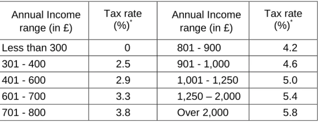
of £1,000.9 This simplicity lasted until 1909; as Table 1 shows, complexity soon set in with a set
of ten marginal rates introduced in 1910 including a top rate of 5.8%.
Table 1 – Income tax rates, 1910-1912
Annual Income range (in £) Tax rate (%)* Annual Income range (in £) Tax rate (%)* Less than 300 0 801 - 900 4.2 301 - 400 2.5 901 - 1,000 4.6 401 - 600 2.9 1,001 - 1,250 5.0 601 - 700 3.3 1,250 – 2,000 5.4 701 - 800 3.8 Over 2,000 5.8 *
Quoted in the tax code in shillings and pence per pound of income
This structure involves the now familiar ‘multi-step tax function’ in which the marginal tax rate (MTR) is changed in discrete ‘steps’ at a set of thresholds covering ranges of income levels – usually, as here, involving progressively rising steps at higher income ranges – but is constant between thresholds. Formally, the multi-step income tax function, with a tax-free income exemption, can be written as:
T(y) = 0 0< y ≤ a1
= t1(y − a1) a1< y ≤ a2
= t1(a2− a1) +t2 (y − a2) a2< y ≤ a3 (3)
and so on, where t and a are the statutory tax rates and income thresholds respectively.
2 . 3 . 2 T h e m u l t i - s l o p e t a x s y s t e m : 1 9 1 4 - 1 9 3 9
The structure in (3) was the structure of the NZ personal income tax system prior to 1914 and from 1940. However, from 1914-1939 the tax schedule involved an increasing tax rate for every
additional pound of income. To distinguish it, we refer to this below as a ‘multi-slope tax
function’ since it involves an upwardly sloping marginal rate function between different income thresholds. In New Zealand it typically applied to incomes in excess of an initial threshold
income level (i.e. a1 in (3) above) and, as an individual’s income increased, the higher rate
applied to all income (above an initial exemption where applicable), not just the increment; see
Vosslamber (2009, p. 304). Thus the apparent marginal rate in the schedule did not specify the ‘effective’ marginal rate since an additional pound of income brought with it an additional tax liability on that pound and all previous pounds above the initial exemption level. In addition, from 1917, this initial exemption level was abated (withdrawn) at £1 for every additional £1 of income
9 Tax rates were expressed as shillings (s) and pence (p) per pound (£) of income, where there were 12 pence per shilling and 20 shillings
in excess of £600, further adding to the ‘true’ marginal rate over this income range.10 This system is described in more detail in Appendix 1.
2 . 3 . 3 O t h e r a s p e c t s o f N e w Z e a l a n d ’ s i n c o m e t a x s t r u c t u r e
It is not possible here to catalogue the numerous changes to the income tax system from 1907 to the present, but a number of milestones in the evolution of the New Zealand income tax structure are worth noting. Those of relevance to AMTR estimates include:
i. The introduction of various exemptions in addition to the ‘general exemption’. These
included exemptions for children and other dependents and a life insurance exemption (see Appendix 3 for details).
ii. The distinction made between earned and unearned income from 1921 to 1950.11 A
10% discount on earned income (up to £2000) was in place until 1930, followed
subsequently by a one-third tax surcharge on unearned income.
iii. A drop in tax rates in the mid-1920s after the WWI ‘temporary’ increases (see Figure 2).
iv. The introduction of a social security tax in 1931 at 1.25%, rising to 12.5% in 1943, then
reduced to 7.5% in 1947 and abolished in 1970.
v. The introduction, also in 1931, of an ‘additional tax’ levy, at 30% of the individual’s
income tax liability. The additional tax was removed in 1936 but re-introduced for
1939-1953. Over the latter period the rate varied subsequently between 2.5% and 33.3%.12
vi. The large increase in EMTRs during WWII with the top rate statutory rate rising to 60%,
and a top EMTR approaching 100% (inclusive of social security and special war taxes).
vii. The replacement of the multi-slope income tax schedule with a multi-step function of
MTRs in 1940 but with 40 separate rates/steps and a maximum statutory rate of 60%.
viii. Generally lower top statutory rates after WWII until the mid-1970s.
ix. Rises in top statutory MTRs to the mid-1980s followed by the sharp drop associated with
the 1980s reforms.
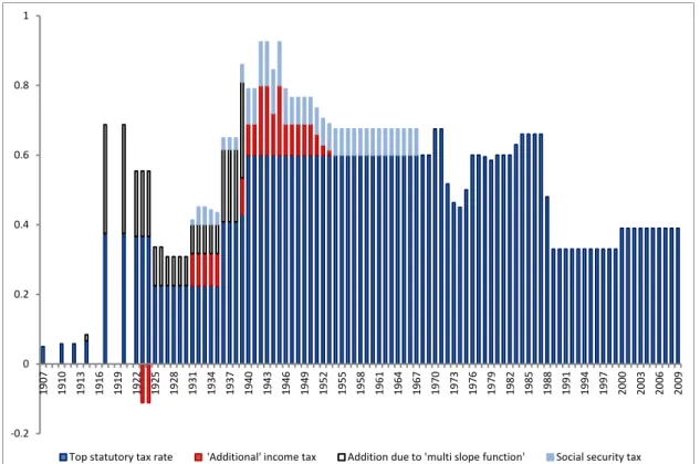
Figure 2 illustrates the decomposition of the top effective marginal tax rate over the period, including the statutory top personal income tax rate plus the ‘additional tax’ component and the social security tax. For the period where the multi-slope function applied, its impact on EMTRs is also shown.
The impact of the ‘additional’ and social security taxes on individual EMTRs is rather different. The relevant expression for an individual’s tax liability can be written as:
T(y) = τ(y – a) + βTI(y) = τ(1 + β )(y – a) (4)
Where τ is the statutory or effective marginal income tax rate, β is the rate of ‘additional tax’
which is applied to the income tax liability, TI, where TI(y) = τ(y – a). The effective marginal tax
rate on income therefore becomes τ(1 + β ). Letting the marginal social security tax rate be s,
the effective marginal tax rate, EMTR, of all taxes combined is composed as follows:
EMTR = s + τ + βτ (5)
10 This abatement regime operated from 1917 to 1926. Two other abatement regimes were in place from 1927-1930 and 1931-1935. More
details are in Appendix 3. A supplementary ‘special war tax’ was also introduced during 1917-20 which effectively applied a multiplier of 1.3333 to all tax rates (e.g. 6% becomes 8%).
11 Earned income was defined as income earned by a taxpayer through physical exertion (largely salary and wage income), whereas,
unearned income relates to passive sources of income such as interest, or rental income.
Here βτ captures the EMTR impact of the ‘additional tax’ levied on the overall income tax liability.
Figure 2 shows how both the social security tax and the additional tax substantially increased effective rates around the WWII period with the additional tax being phased out in the mid-1950s. The social security tax was retained till the late-1960s. For four years during WWII the combined effect of all three taxes produces a top EMTR in excess of 90%: a top IT = 60%;
additional tax = 20% (i.e. legislation set β = 0.33 in those years) and SST = 12.5%.
During the 1920s-30s, the impact of the multi-slope tax schedule on top EMTRs was also substantial, often adding around 15-20 percentage points to those specified in the tax schedule. These high effective rates typically applied at high, but not the highest, income levels (see Appendix 1). In 1923 and 1924 there was a 20% discount on the tax bill, resulting in net a top EMTR of 44%.
Figure 2 – Top effective marginal tax rates for New Zealand, 1907-2009*
* Tax rates shown include social security taxes and relate to earned income where relevant.
Finally, for much of the period studied the amount of tax that individuals paid was also dependent on the amount of exemptions received, which reduced their average tax rates.
These can affect individuals’ effective marginal tax rates directly when they are abated with
rising incomes, as discussed above, and indirectly by affecting the number of income earners liable to tax, their assessable income and hence the statutory marginal tax rates applicable for a given gross income. They therefore would shift some individuals across tax brackets and affect
economy-wide AMTRs as discussed in section 4.
3
N e w Z e a l a n d I n c o m e D i s t r i b u t i o n D a t a
To calculate aggregate level AMTRs requires suitable income distribution data to enable the income-weights to be generated. Income distribution data used here for the purpose of
-0.2 0 0.2 0.4 0.6 0.8 1 19 07 19 10 19 13 19 16 19 19 19 22 19 25 19 28 19 31 19 34 19 37 19 40 19 43 19 46 19 49 19 52 19 55 19 58 19 61 19 64 19 67 19 70 19 73 19 76 19 79 19 82 19 85 19 88 19 91 19 94 19 97 20 00 20 03 20 06 20 09
estimating AMTRs have largely been sourced from the New Zealand Official Yearbooks
(NZOYB), which in turn were sourced from income tax returns filed with Inland Revenue. We have been able to identify data from the early 1900s through to the early 1980s and over this period the data presented in the NZOYBs have evolved. Income data were not separately sourced after the early 1980s. Instead we have utilised AMTRs estimated from more reliable unit record data by Inland Revenue for the period 1981-2009, and we examine a three year overlap as a cross-check on the alternative approaches.
3 . 1
I n c o me D a t a
There are three important aspects to the income distribution data for our purposes:
1. how income is distributed across the tax brackets/rates for which we have tax schedule information;
2. how exemptions against tax are distributed across income levels and tax brackets; and 3. how far NZOYB income distribution data, generally only available for tax filers until the
PAYE regime from 1958, can be supplemented to capture non-filers’ incomes.
We assembled NZOYB income data on individual taxpayers (for example, wage and salary earners, and self employed), but excluding companies. We focus on the distribution of income for aggregate gross income (before exemptions), aggregate earned and unearned income, and
income tax exemptions.13 We also used data on the number of tax returns filed to estimate the
size of non-filed income (see below).
Of course, available income and tax data vary in quality and coverage over the period of the personal income tax, and we have found no suitable income data prior to 1907. Appendix 2 discusses the nature and quality of the income data over various sub-periods during 1907-1983, highlighting the main methods and assumptions adopted.
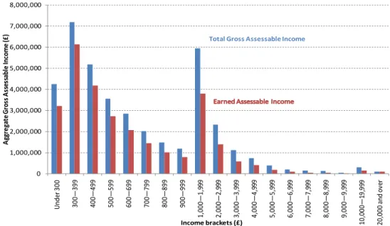
Figure 3 provides an example of how the income distribution data are organised, in this case for 1925. It shows total assessable income, not numbers of taxpayers, on the vertical axis, with income classes on the horizontal, where the class widths are not standardised. The distribution of gross assessable income is shown with separate histograms for total, and earned, income. Where tax brackets do not coincide with the relevant income classes, aggregate income within the income class is divided on a pro rata basis to allow each segment to be taxed at the appropriate rate. Note that the spike in income in bracket 1,000-1,999 is due to the larger size of this and subsequent brackets.
In 1925, earned income below a certain threshold was taxed at a lower rate compared to
unearned income (applicable through the first half of the 20th century). In addition, certain
income was exempt from tax depending on a taxpayer’s circumstances. Data on tax exemptions, distributed by size of income, first appeared in the NZOYB in this period and are described further in Appendix 3.
13 The NZOYB also has data on taxable income (i.e. gross income less exemptions), income tax assessed, and similar measures of income
and tax for companies. The NZOYB ceased publishing final income data from 1973, though provisional estimates of income were included. Instead, for the 1970s and early 1980s we source income and exemption data from the separate SNZ Report on Incomes and
Figure 3 – Distribution of total and earned assessable income, 1925
3 . 2
E x e mp t i o n s D a t a
Until the 1970s exemption of some income from personal income tax was a feature of the New Zealand tax system. A portion of income was exempt from tax for a specified set of circumstances, including: low income (the ‘general exemption’), and exemptions for child/dependent, wife/spouse, housekeeper and insurance (related to life insurance and superannuation fund contributions). This had the effect of reducing individuals’ tax liabilities, for given gross income, depending on their individual circumstances, thereby affecting their
average tax rates. It directly affected their effective marginal tax rates to the extent that exemptions were income-dependent (e.g. were withdrawn in association with increasing income). It would also have affected the relevant statutory tax rate where exemptions shifted a taxpayer between MTR bands. In Appendix 3 we describe the exemptions data further and section 4 below discusses how we use data on the distribution of exemptions by income levels in the AMTR calculations.
3 . 3
N o n - F i l e r I n c o me s
A major omission from NZOYB income data is the income of individuals who were not required to file tax returns, prior to the introduction of PAYE in 1958. Non-filers were generally those with incomes below the low-income ‘general exemption’ threshold since those with incomes above this level were legally required to file a return. Appendix 4 describes the methods we use to estimate the income of non-filers. While omission of these non-filers with a zero EMTR would not be a problem for calculations of a tax-share weighted estimate of the aggregate AMTR, it is potentially important for an income-weighted average. Ignoring non-filers would risk over-estimating the AMTR.
In brief, our method of estimating non-filers’ income involves using census data for 1926, 1936, 1945 and 1951 and labour market data to derive estimates of total personal incomes which can be compared with our NZOYB data on filers’ total personal incomes. One option would be to interpolate between census years using the ratio of filer-to-all personal incomes. This ratio
0 1,000,000 2,000,000 3,000,000 4,000,000 5,000,000 6,000,000 7,000,000 8,000,000 Un de r 3 00 30 0— 39 9 40 0— 49 9 50 0— 59 9 60 0— 69 9 70 0— 79 9 80 0— 89 9 90 0— 99 9 1, 00 0— 1, 999 2, 00 0— 2, 999 3, 00 0— 3, 999 4, 00 0— 4, 999 5, 00 0— 5, 999 6, 00 0— 6, 999 7, 00 0— 7, 999 8, 00 0— 8, 999 9, 00 0— 9, 999 10 ,0 00 — 19 ,9 99 20 ,0 00 an d o ve r Ag gr eg at e G ro ss A ss ess ab le In co m e ( £) Income brackets (£)
reveals an increasing trend, rising from 0.347 (for 1926) to 0.707 (1936), 0.919 (1945) and 0.963 (1951).
However, evidence from Barro and Sahasakul (1983) suggests that, while this ratio tends to trend up over time in association with rising income levels, it can be especially low during short-run recessionary periods. Within our dataset, this includes the 1920s-30s depression when large falls in personal incomes reduced the numbers of those required to file. Data on GNP are available throughout our period of interest, and this could be expected to capture recessionary impacts.
We therefore estimate the ratio of total personal income, Y, to GNP in Census years
(subscripted ‘c’), Yc,/GNPc, and use interpolated (subscripted ‘i’) values of this ratio, and annual
GNP values, to estimate values of Yi for non-Census years. Together with our estimates for
total income of filers, Y(F)i, for those years we can estimate filers incomes, Y(N), in
non-Census years as Y(N)i = Yi - Y(F)i. The resulting time-series for the ratio of filers-to-total
income, and the decomposition of total income into filer/non-filer categories, are shown in Appendix 4, Figures A3 and A4 respectively. These suggest a plausible but fluctuating fall in the extent of non-filers’ incomes, reaching less than 4% of total personal incomes by 1951.
4
C a l c u l a t i n g A M T R s – M e t h o d o l o g y
4 . 1
A p p l y i n g t h e B a r r o - S a h a s a k u l Ap p r o a c h
As noted in the introduction, the AMTR of interest here is the Barro and Sahasakul (1983) income-weighted average of individual effective marginal personal income tax rates. That is, we want to estimate the aggregate:
𝐴𝐴𝐴𝐴𝐴𝐴𝐴𝐴 =� �YYj�EMTRj
𝑛𝑛
𝑗𝑗=0
(6)
where Yj is the personal income of taxpayer j, and Y is aggregate personal income across all j
taxpayers. The EMTRjs are obtained from the tax schedule or suitably adjusted ‘effective’ rates
where those differ from statutory rates. The relevant tax rates and thresholds are then matched
with information on (Yj/Y) from our income distribution data, inclusive of the income share of
non-filing taxpayers. To avoid confusion, in the remainder of the paper we refer to marginal tax
rates (MTR, EMTR) levied at the individual level using the subscript j; hence: MTRj, EMTRj.
Applying equation (6) to our data requires a number of simplifying assumptions. Firstly, from
1981-2009 the use of taxpayer unit record data ensures that the relevant MTRj or EMTRj of
income tax is identified for each taxpayer. However, like the pre-1981 data, this dataset does
not include the impact on EMTRjs of abatement of social welfare payments.
For data prior to 1981, we seek to match data from NZOYB and other sources on the distribution of gross assessable income with the relevant tax schedule. Since tax brackets are
typically described with respect to net-of-exemptions assessable income, it is important to
subtract those exemptions to identify net income and thereby the appropriate EMTRj to apply at
each gross income level. For many taxpayers, the deduction of exemptions from their gross
$50,000 will not affect the MTRj where this MTRj applies over a net income band of
$40,000-50,000. However, another taxpayer with the same $50,000 of gross income but $12,000
exemptions would face a different MTRj - that applicable to net income below $40,000.
We therefore need to deduct exemptions from gross (assessable) income to derive net
(assessable) income in order to identify the relevant MTRj or EMTRj for each taxpayer.
However, with aggregate-level, rather than individual-level, gross assessable income and exemptions data by gross income band, we do not know how many taxpayers (and associated fraction of gross income) would face a lower marginal tax rate than would be inferred from their gross income.
Treating our aggregate-level data as if they represented an individual within each income band
would mean that either all or no income would shift MTRj bands as a result of adjusting for
exemptions. Instead we (i) assume that the impact of exemptions is to move individuals by no
more than one MTRj band; and (ii) use the ratio of total exemptions to gross assessable income
in each band to weight the MTRjs for each band, m. This yields an EMTRj estimate reflecting
the exemptions adjustment:
EMTRj,m = (em/ym) MTRj,m-1 + (1 - em/ym) MTRj,m (7)
Where (em/ym) is the exemptions/income ratio in band m, and MTRj,m (MTRj,m-1) is the MTRj in
band m (m-1), (m > 0) and MTRj,0 = 0, captures the general personal exemption. To examine
the sensitivity of our AMTR calculations to this assumption, we also report AMTRs where no
shifts in MTR brackets, based on exemptions data, has been assumed.
4 . 2
E x a mp l e s o f A M T R c a l c u l a t i o n s
Table 2 shows an example of the AMTR calculations – for the 1980 income year – when there
were relatively few (six) income tax brackets and MTRjs. Since the income tax schedule defines
taxable income as income net of exemptions (deductions), the income brackets in row 1 are defined with respect to net income.
Table 2 – The AMTR calculations, 1980
1. Taxable income bracket ($) <4,500 4,500-10,000 10,000-11,000 11,000-16,000 16,000-22,000 >22,000 Total 2. Statutory MTR 14.5% 36.5% 41.5% 48.0% 55.0% 60.0% 3. EMTR 13.5% 35.2% 41.2% 47.6% 54.6% 59.8%
4. Gross assess-able income 1,225,465 4,565,695 991,170 3,550,580 1,583,880 1,304,220 13,221,010
5. Exemptions 85,775 275,315 66,130 235,960 90,860 45,870 799,910
6. income share (%) 9% 35% 7% 27% 12% 10% 100%
Income-weighted AMTR = 41.70%
The MTRj for each income bracket is shown in row 2. Row 3 provides an estimate of the
EMTRj faced by individuals in each tax bracket, adjusted for the impact of exemptions.14 This
adjustment weights the MTRjs in each bracket by the ratios of exempt income (row 5) to gross
income (row 4). For example, approximately 7% of income in the <4,500 bracket in 1980 was
exempt from tax; we therefore assume that this fraction of income faces the MTRj of the bracket
immediately below; in this case, 0%. In view of the small amount of exemptions (averaging 6% of gross income), the resulting impacts on the 1979/80 EMTRs in row 3 are small.
14 Note that this is not an EMTR as conventionally defined since no individual faces this rate. Rather it reflects the weighted average of rates
The relevant gross income shares are calculated in row 6. In principle, non-filer income is also added before estimating the gross income shares in row 6 though, as noted above, this is not
relevant after 1958. Applying the row 6 weights to the EMTRjs in row 3 yields the AMTR
(=41.70%) for 1980. It can be seen that this is dominated by the large shares (nearly 65%) of
income in the $4.5-10k and $11-16k income brackets facing EMTRjs of 35.2% and 47.6%
respectively.
The case in Table 2 illustrates a relatively straightforward year. Most years, however, involve multiple marginal tax rates across income levels and a variety of additional complications including:
i. earned and unearned income distinctions (1921-50) with each facing different MTRjs15
ii. estimation of EMTRjs where statutory rates do not measure effective rates; e.g.
separate non-filer incomes and abatement of thresholds
iii. The multi-slope tax function where EMTRjs rise with every pound of income (1914-39);
in that case we calculate AMTRs based on EMTRjs at the mid-points in income classes
across the income distribution
iv. income classes from income distribution data that approximate the income bands in the
tax structure, requiring some re-grouping of data on incomes, exemptions etc.
v. simultaneous application of several different taxes at various rates to a given income
including social security taxes, and special ‘war taxes’
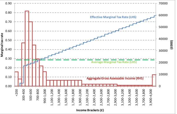
Figure 4 – Income distribution and tax structure, 1950
Figure 4 illustrates the more complex 1950 income distribution and tax structure. This overlays
income distribution data with the individual EMTRjs. The rates rise in multiple steps from 4% at
an income of £200 to 76% at incomes over £4000. This yields the AMTR of 29% shown.
Exemptions data are used to adjust the EMTRjs to approximate the effect of people moving to
lower income brackets. This adjustment has a particularly large impact at the bottom of the income distribution; for the £200-300 bracket the effective tax rate drops from 21%, before
15 Data on earned incomes was collected until 1956 but earned and unearned income faced the same tax rate from 1951-1956.
0 10000 20000 30000 40000 50000 60000 70000 0.00 0.10 0.20 0.30 0.40 0.50 0.60 0.70 0.80 0.90 <2 00 30 0-40 0 50 0-60 0 70 0-80 0 90 0-1, 00 0 1, 10 0-1, 20 0 1, 30 0-1, 40 0 1, 50 0-1, 60 0 1, 70 0-1, 80 0 1, 90 0-2, 00 0 2, 10 0-2, 20 0 2, 30 0-2, 40 0 2, 50 0-2, 60 0 2, 70 0-2, 80 0 2, 90 0-3, 00 0 3, 10 0-3, 20 0 3, 30 0-3, 40 0 3, 50 0-3, 60 0 3, 70 0-3, 80 0 3, 90 0-4, 00 0 (£ 00 0) M ar gi nal tax rat e Income Brackets (£)
Effective Marginal Tax Rate (LHS)
allowing for exemptions, to 4%. That is, the availability of exemptions shifts a large fraction of taxpayers into the 0% tax rate applied to net incomes up to £200.
5
I n c o m e - w e i g h t e d A M T R s : 1 9 0 7 - 2 0 0 9
Using the tax structure and income distribution information discussed in previous sections, this section discusses the estimated values obtained using the methods described earlier – sub-section 5.1. Since the relationship between exempt and non-filer incomes is important for these calculations, this is discussed in sub-section 5.2. Sub-section 5.3 then uses a decomposition of the AMTRs to assess how far changes in tax structure and income levels or its distribution account for observed movements in AMTRs over time.
5 . 1
T h e Ov e r a l l p a t t e r n o f A MT R s
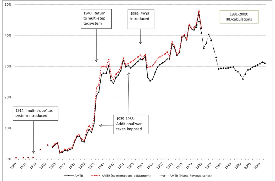
The changes in both the tax schedule and income distribution over the period from 1907 to 2009 have resulted in an AMTR series which varies substantially over the period. Figure 5
shows two AMTR series. The main series (in black) uses exemptions data to adjust the EMTRjs
up to 1983, and reports IRD-based calculations from 1981. This series is also given in Table 3.
A second series ignoring exemptions data (that is, individual EMTRjs are not adjusted using
exemptions data) is shown in dotted red.
Both series ranges from 0.4% in 1907, the first year for which income distribution data are available, to a maximum of around 47% in 1982. It can be seen that in general the two series follow each other closely suggesting that exemptions adjustments play a limited role. The main period during which exemptions adjustments have a larger impact is 1954 to 1969. As discussed below, this was a period that witnessed a substantial increase in the initial tax-free allowance and other exemptions.
Based on the main series, the AMTR increases during WWI and its aftermath, reaching 5.4% in 1924. It then drops back to 2-3% in the second half of the decade. Thereafter during the inter-war period, the AMTR rises especially during the years of the Great Depression from 1929, reaching a maximum of 7.4% in 1933.
The most significant increase in the AMTR over the century, however, occurs at the beginning of WWII where the rate jumps from 11% in 1939 to 21% in 1940. The AMTR continues to rise thereafter to reach a local maximum of 30% in 1945. Though the AMTR drops in the immediate aftermath of the war, the lower AMTRs over the remainder of the decade are short-lived with an increase to 32% by 1951. Changes to the tax system from 1939 to 1953 were largely enacted through the use of additional war-related income taxes, ranging from an additional 2.5% to 33% added to individuals’ final income tax bills. These had the administrative advantage of raising extra revenue without needing to adjust the basic income tax schedule; see Vosslamber (2009). After WWII the AMTR appears to follow a fairly steady upward trend till 1982, interrupted by two substantial declines: in 1961 and in 1971-3. Both declines largely reflect tax structure, mainly rate, changes but whereas the 1971-3 rate reductions mainly involved declines in top rates (see Figure 2), the 1961 case primarily reflected cuts in lower tax rates and increased exemptions. Both reductions in AMTRs were soon reversed, with exemptions subsequently curtailed in the
mid-1960s, and the removal of the general personal exemption plus increased MTRjs in 1975
as the early 1970s oil crisis hit. Section 5.3 discusses the decomposition of AMTR changes in more detail.
Figure 5 – AMTRs for New Zealand 1907-2009 0% 10% 20% 30% 40% 50%
AMTR AMTR (no exemptions adjustment) AMTR (Inland Revenue series)
1959: PAYE introduced 1914: 'multi-slope'tax system introduced 1940: Return to multi-step tax system 1939-1953: Additional 'war taxes' imposed 1981-2009: IRD calculations
Table 3 – Average marginal tax rates (in percent), 1907-2009
Year AMTR (%) Year AMTR (%) Year AMTR (%)
1907 0.4 1941 21.7 1975 39.3 1908 - 1942 27.3 1976 39.9 1909 - 1943 27.8 1977 38.5 1910 0.4 1944 27.7 1978 43.3 1911 - 1945 30.2 1979 42.1 1912 0.5 1946 25.4 1980 41.7 1913 - 1947 24.4 * 1981 42.6 1914 0.5 1948 26.3 1982 44.6 1915 - 1949 27.1 1983 40.9 1916 - 1950 28.7 1984 35.9 1917 3.0 1951 32.0 1985 37.5 1918 - 1952 29.8 1986 40.4 1919 - 1953 30.1 1987 38.6 1920 4.5 1954 29.5 1988 35.8 1921 - 1955 30.1 1989 33.0 1922 3.7 1956 30.8 1990 29.2 1923 4.6 1957 31.5 1991 29.5 1924 5.1 1958 32.4 1992 29.5 1925 1.9 1959 32.1 1993 29.4 1926 2.2 1960 33.3 1994 29.6 1927 2.8 1961 26.4 1995 29.7 1928 2.6 1962 25.2 1996 29.9 1929 3.1 1963 25.8 1997 28.7 1930 3.3 1964 27.8 1998 28.3 1931 5.5 1965 29.7 1999 27.2 1932 7.2 1966 30.5 2000 26.0 1933 7.4 1967 31.1 2001 27.6 1934 5.8 1968 31.4 2002 28.9 1935 5.5 1969 32.4 2003 29.1 1936 8.0 1970 32.4 2004 29.7 1937 9.6 1971 37.1 2005 30.2 1938 8.7 1972 35.9 2006 30.5 1939 11.3 1973 33.4 2007 30.9 1940 20.5 1974 34.4 2008 31.3 2009 31.1 * Data from 1981 are sourced from Inland Revenue
Following the early 1980s peak around 47%, a substantial decline in the AMTR occurs, in part associated with the familiar ’80s reforms, though beginning prior to the main mid-1980s reform years, and falling to around 30% by 1990. The data also confirm a decline in the AMTR during 1996-2000 in association with revenue-reducing tax reforms (e.g. the
lowest MTRj fell from 24% in 1994 to 19.5% in 2000, and thresholds were raised). This
the increase in the top MTRj from 33% to 39% in 2000, and the resulting impact of fiscal
drag thereafter as income tax thresholds remained fixed in nominal terms.16
Comparing the two series in Figure 5 reveals the impact of our ‘exemptions adjustment’ designed to capture the effect of general exemptions reducing net, relative to gross, income. As noted above, for an (unknown) fraction of taxpayers, this would reduce the statutory marginal tax rate that they faced. It can be seen that the adjustment has little effect on estimated AMTRs except for the early 1940s, 1954-58 and 1961-69. For the first two period AMTRs are reduced by about 1-2 percentage points (ppt); during 1961-69 the
difference in the series ranged from almost 5 ppt (1962) to 2.4 ppt in 1969. In each of these cases tax structure changes in 1940, 1954 and 1962 involved an increase in the initial income level liable to the 0% marginal tax rate, hence affecting the fraction of
taxpayers who may face a lower MTRj. Year-to year changes in the two series are
however largely unaffected by the adjustments.
Finally, the AMTR calculations described here exclude the impact of ACC levies, the Benefit system and the Family Tax Credit (FTC) system which, at various times since the 1970s, involved lump sum transfers to lower income families with children that were withdrawn at higher income levels at rates of up to 30c/$, thereby adding to effective
MTRjs. The effect of FTCs is discussed further below.
5 . 2
R e l a t i o n s h i ps be t w e e n E x e mp t i o n s , N o n - F i l e d
I n c o me s a n d A M T R s
The calculated AMTRs incorporate estimates of the amount of income exempt from tax, including income which was not required to be filed with the tax department, and its impact on the effective marginal tax rate faced by individuals. Non-filer income is effectively treated as being ‘taxed’ at a zero tax rate in our calculations, and this has a significant impact in lowering the AMTRs. For exempt income we have sought to capture the impact of exemptions in moving people to lower marginal tax brackets as discussed above. This had a smaller, but nevertheless noticeable impact, especially where it moves some taxpayers into a tax-free income bracket.
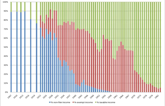
Figure 6 shows how the proportions of exempt and non-filer income changes over the 1907 to 1982 period. (This is not readily calculated for the post-1982 IRD dataset). During
the early part of the 20th century, we estimate that a large proportion of income was not
filed. In 1907, approximately 89% of income was not filed because it fell under the £300 filing limit. This proportion reduced steadily throughout the first half of the century, and by 1958 when the PAYE system was introduced it was close to zero. As described above, there were a number of tax exemptions available. The proportion of income which was exempt from tax is shown in red in Figure 6. By 1980 income exempt from tax represented only around 5% of gross assessable income.
Figure 6 – Proportions of taxed, exempt and non-filed income, 1907 – 1983
5 . 3
D e c o mp o s i n g C h a n g e s i n t h e A MT R s
The variations in the AMTR over the period can be decomposed into changes to the tax system, changes in average income levels, and changes to the income distribution. The impact of each of these varies across the period. This section attempts to identify the most significant impacts in different time periods.
The AMTRs changed only slightly during the period 1907 – 1916, due to minor changes in both tax rates and income distribution. In 1914 the multi-slope scale was introduced. It did not have a large impact on the AMTR, however, as the tax rates remained low and there were many unaffected non-filers.
In 1917 effective marginal tax rates were increased substantially (by around 3 times at the lower end of the income distribution and up to 8 times at the upper end). The increase included the addition of a ‘special war tax’. In addition, abatement of the general exemption was introduced. As a result the AMTR increased from 0.5% in 1914 to 3.0% in 1917. It increased further to 4.5% in 1920, solely as a result of increasing incomes which moved people into higher tax brackets (the tax system did not change). From 1922 to 1924 tax rates were reduced slightly, but the AMTRs continued to rise due to increasing incomes shifting the distribution towards higher income tax brackets.
It was not until 1925, however, that post-WWI tax rates fell more significantly, with the top marginal tax rate dropping from 29% in 1924 to 22.5% in 1925. Thereafter the AMTR generally rose slowly over the remaining ’20s and ’30s, except for a relatively large rise (compared to previously) between 1930 and 1932. This largely reflected tax schedule
changes in 1931.17 In the same year, total income dropped by 5% and the income
17 For example, the statutory MTRjs were approximately doubled across the income distribution and the tax-free threshold was
reduced; a 30% additional tax was added to the final tax bill; social security tax was introduced at 1.25%; and a supplementary 0% 10% 20% 30% 40% 50% 60% 70% 80% 90% 100%
distribution was skewed downwards. The net effect of these changes was an increase in the AMTR from 3.3% in 1930 to 5.5% in 1931.
From the mid-1930s to the early post-WWII years, AMTRs rose rapidly and did so again from the mid-1970s until the early 1980s. In between, the roughly 30 year period from the mid-1940s to mid-1970s reveals a steady upward trend the AMTRs, punctuated by a brief decline from 1951-54 and the sharp fall in 1961-63.
The especially rapid rise in the lead-up to, and during, WWII largely reflects tax system changes: mainly tax rate and threshold changes designed to raise additional revenue. In 1936 tax rates were increased substantially (the top marginal rate on earned income increased from around 43% in 1935 to 65% in 1936), and increased again in 1939 plus an “additional tax” at 15% to finance the war effort (War Expenses Act 1939). In 1942 social security was increased to 12.5% and the additional tax was increased from 15% to 33.3%. Combined with an upward movement in incomes, these changes generated a rise in the AMTR to 27% in 1942 and 30% by 1945.
Unsurprisingly, the sharp drop in the AMTR in 1946 captures the reduction in social security and the additional ‘war’ tax to 10% and 15% respectively in the aftermath of the war. However, as noted above, upward movements from 1948 are interrupted by reductions in 1951-54 and 1961-63. Both appear to arise mainly from legislated increases in exemptions. The large drop in 1962-63 reflects both increased generosity of exemptions (they rose from 46% of total gross assessable income in 1961, to 56% in
1963) and across-the-board upward shifts in MTRj thresholds in 1962.
The upward trend in the AMTR was interrupted briefly in the early-1970s and halted sharply in 1982 – well before the major economic and tax reforms of the mid-1980s. As with the AMTR declines in 1962-63, the decline in AMTR from 1982-84 is associated with increases in the tax thresholds at most income levels (but a new higher top rate) and some schedule simplification in 1984. The major reforms involving a reduced top rate did
not become effective until 1988-89 when the top MTRj was reduced from 66% in 1987 to
48% in 1988 and 33% in 1989.
Further insight into the time-series pattern of AMTRs, and the role of different components, can be obtained by considering the relationship between personal income
not subject to income tax and the AMTR. Figure 7 shows cross-plots of the AMTR with the
estimated income share of non-filers. It also shows the share of income (of filers) that is tax-exempt – where the latter is added to the former in Figure 7. Increasing exemptions push more taxpayers into tax-free status (when an initial zero tax rate exists) as well as
reducing positive MTRjs for others.
The Figure shows the time-series from 1922 (top left corner) to 1983 (bottom right corner)
with dashed lines joining annual observations.18 The non-filers’ share reaches zero (in
1958) and therefore tracks the horizontal axis thereafter. The non-filers’ income share reveals a clear negatively-sloped, and non-linear, relationship with the AMTR, - the correlation with the AMTR is -0.91 (1922-58). The relationship of the AMTR to exemptions
is more complex. Though the combined ‘non-filers plus exemptions’ share in Figure 8
reveals a negative slope, for exemptions alone the correlation with the AMTR is +0.76 (1922-58) but -0.93 (1959-83). That is, as AMTRs generally rose over time, and non-filing became less common (to 1958), exemptions tended to replace non-filing as the preferred means of keeping tax rates low or zero on lower income earners. After 1958 however, when PAYE was introduced, exemptions tend to decline over time in association with rising AMTRs.
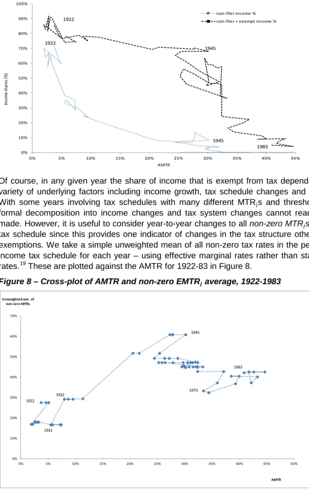
Figure 7 – AMTRs and tax exempt/non-filed income, 1922-1983
Of course, in any given year the share of income that is exempt from tax depends on a variety of underlying factors including income growth, tax schedule changes and so on.
With some years involving tax schedules with many different MTRjs and thresholds, a
formal decomposition into income changes and tax system changes cannot readily be
made. However, it is useful to consider year-to-year changes to all non-zero MTRjs in the
tax schedule since this provides one indicator of changes in the tax structure other than exemptions. We take a simple unweighted mean of all non-zero tax rates in the personal income tax schedule for each year – using effective marginal rates rather than statutory
rates.19 These are plotted against the AMTR for 1922-83 in Figure 8.
Figure 8 – Cross-plot of AMTR and non-zero EMTRj average, 1922-1983
19 That is, social security, additional taxes/discounts and exemption adjustments are included. Using statutory rates yields similar 0% 10% 20% 30% 40% 50% 60% 70% 80% 90% 100% 0% 5% 10% 15% 20% 25% 30% 35% 40% 45% In co m e sh ar es (% ) AMTR non-filer income % non-filer + exempt income %
1983 1945 1922 1922 1945 0% 10% 20% 30% 40% 50% 60% 70% 0% 5% 10% 15% 20% 25% 30% 35% 40% 45% 50% Unweighted ave. of non-zero MTRs AMTR 1922 1945 1973 1983 1931 1932
This reveals that the rise in the AMTR occurred largely in association with a rise in the
‘average’ non-zero MTRj that each individual faced in the tax schedule from around 1931
(bottom left corner), until around 1942-45 but not thereafter. That is, for the post-WWII period, increases in the AMTR are not generally associated with changes to the tax
schedule that raised MTRjs, though this does not of course preclude changes in
thresholds that meant a given MTRj applied at higher or lower income levels. In essence,
by the 1940s, top (and other) MTRs had reached sufficiently high levels, that they tended to remain around those levels or fall back in subsequent years.
Though these broad patterns over several years are revealing they do not indicate the extent to which each annual change in the AMTR reflects its various components. To apply that here, for the 1907-2009 period, first consider a simplified two-rate step function
involving two tax rates, t0, t1, where t0 = 0, and t1 > 0. For this simplified case the change
in the AMTR, dM, can be broken down into:
dM = w1dt1 + t1dw1 + dt1dw1 + { w0dt0 + t0dw0} (8)
where w1 is the income weight of taxpayers facing t1 (= 1- w0), and the term in curly
brackets is zero (t0 = dt0 = 0). The income weights are affected by tax thresholds that
determine the MTRjs applicable at different taxpayer income levels. Of course the NZ
personal income tax schedule involves a more complex structure of several (sometimes many!) non-zero tax rates. Nevertheless it is useful to approximate the exact specification
in (8) using the annual ‘unweighted average’ of the non-zero MTRjs, in the schedule, as
shown in Figure 8. Thus (8) becomes:
dM = w’1dt’1 + t’1dw’1 + dt’1dw’1 + R (8’)
where t’ is the simple average of non-zero MTRjs in the schedule, w’ is the income weight
of all taxpayers facing a non-zero MTRj, and R is a residual – capturing the omitted
components involving changes in each non-zero MTRs relative to the average t’1,
changes in associated tax thresholds, and changes in income shares relative to w’1.
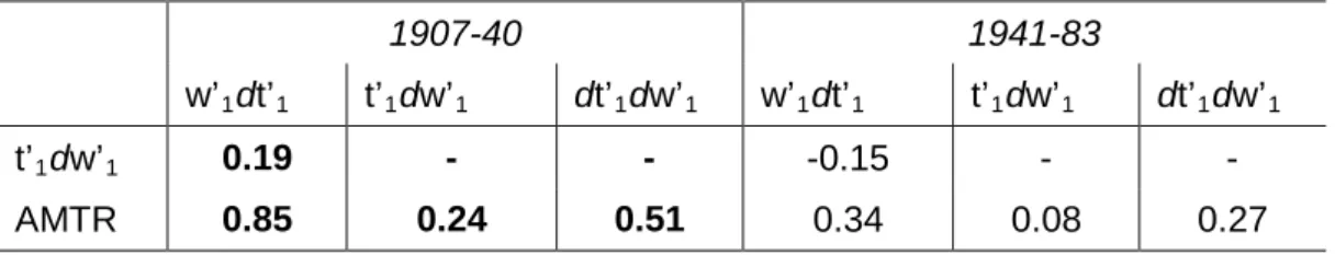
Using (8’) to decompose changes in AMTRs (dM) for each year during 1907-83 gives the
following correlation matrix where pre- and post-1940 correlations are examined separately – Figure 9 suggests a different relationship after around 1940.
Table 4 – Correlation matrix of AMTR changes
1907-40 1941-83
w’1dt’1 t’1dw’1 dt’1dw’1 w’1dt’1 t’1dw’1 dt’1dw’1
t’1dw’1 0.19 - - -0.15 - -
AMTR 0.85 0.24 0.51 0.34 0.08 0.27
It can be seen that both changes in the share of taxable in total income, t’1dw’1, and
changes in ‘average’ non-zero MTRjs, w’1dt’1, are positively correlated with annual
changes in the AMTR. However changes in the taxable income share have a much smaller correlation at 0.24 versus 0.85 (pre-1940) and 0.08 versus 0.34 (post-1940). The
positive cross-correlation between, w’1dt’1 and t’1dw’1 reveals that this has a larger effect
on the AMTR than the change in the income weight, t’1dw’1.
These correlations therefore reinforce the view that, at least to around 1940, the annual
AMTR changes were largely associated with changes in the set of non-zero EMTRjs –
both directly and via the associated change in income weights (due to dt’1dw’1). By
themselves change in the income weighting (between taxed and untaxed incomes) within the AMTR calculation had relatively little impact. After 1940 changes in average non-zero
tax rates are still important but other factors (hidden within the residual in equation (8’)) appear to be more important.
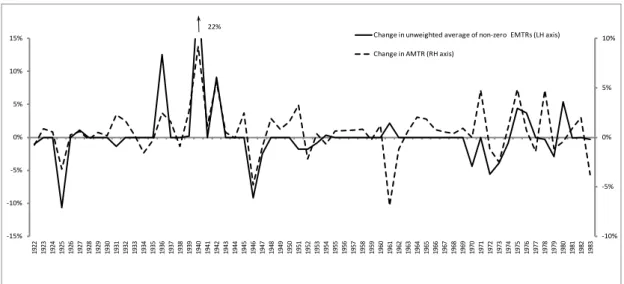
The data underlying these correlations can be seen in Figure 9, which plots the annual
change in the AMTR (right-hand axis) and the unweighted average non-zero EMTRjs
(left-hand axis). This reveals that for many years the EMTRjs remain relatively constant
(generally because statutory rates are unchanged), while the AMTR changes - because of changes to income levels/distribution, changes in thresholds, exemptions etc. Nevertheless, many of the largest changes in the AMTR are associated with substantial changes in statutory or effective marginal tax rates such as in 1925, 1936, 1940-42, 1946 and the 1970s.
Figure 9 – Changes in unweighted averages of EMTRjs and AMTRs, 1922-1983
5 . 4
E a r n e d v s . U n e a r n e d I n c o me
As noted above, throughout the period from 1922 to 1949 a distinction was made between earned and unearned income and these were taxed at different rates. Figure 10 shows the AMTRs for earned and unearned income, as well as the total AMTR. Up until 1930 the tax rate on earned income was reduced by 10% (relative to that for unearned income) for the first £2000 of income. During this period the AMTRs for the two types of income tracked each other fairly closely, with the AMTR for unearned income generally at 2% to 5% above that on earned income.
From 1931 to 1949 the distinction was changed such that the tax on unearned income was increased by 33.3% relative to that on earned income. From 1939 the gap between the unearned AMTR and earned AMTR begins to increase, reaching its greatest divergence in 1945 with a gap of 24 percentage points. This widening gap is due exclusively to the changing relative income distributions of earned and unearned income. The proportion of unearned income at the top end of the income distribution increased dramatically during this period. For example, the proportion of unearned income in the top bracket (>£4000) increased from 2% in 1940 to 17% in 1945, while the proportion of earned income in this top bracket remained fairly constant at around 1%.
Unsurprisingly, the overall AMTR is driven mostly by the AMTR for earned income reflecting the low share of unearned income in total income. Moreover, this proportion decreased substantially over the period, such that the very large AMTRs for unearned income in the mid 1940s did not have such a large impact on the overall figure. Unearned income made up around 40% of all filers’ income in the early 1920s, but had dropped to around 4% by 1949, the last year in which the two were taxed at different rates. Indeed
-10% -5% 0% 5% 10% -15% -10% -5% 0% 5% 10% 15% 1922 1923 1924 1925 1926 1927 1928 1929 1930 1931 1932 1933 1934 1935 1936 1937 1938 1939 1940 1941 1942 1943 1944 1945 1946 1947 1948 1949 1950 1951 1952 1953 1954 1955 1956 1957 1958 1959 1960 1961 1962 1963 1964 1965 1966 1967 1968 1969 1970 1971 1972 1973 1974 1975 1976 1977 1978 1979 1980 1981 1982 1983 Change in unweighted average of non-zero EMTRs (LH axis) Change in AMTR (RH axis)