Two Stage Robust Ridge Method in a Linear Regression Model

Volume 14 | Issue 2 Article 8

11-1-2015

Two Stage Robust Ridge Method in a Linear

Regression Model

Adewale Folaranmi Lukman

Ladoke Akintola University of Technology, [email protected]

Oyedeji Isola Osowole

University of Ibadan, [email protected]

Kayode Ayinde

Ladoke Akintola University of Technology, [email protected]

Follow this and additional works at:http://digitalcommons.wayne.edu/jmasm

Part of theApplied Statistics Commons,Social and Behavioral Sciences Commons, and the

Statistical Theory Commons

Recommended Citation

Lukman, Adewale Folaranmi; Osowole, Oyedeji Isola; and Ayinde, Kayode (2015) "Two Stage Robust Ridge Method in a Linear Regression Model,"Journal of Modern Applied Statistical Methods: Vol. 14 : Iss. 2 , Article 8.

DOI: 10.22237/jmasm/1446350820

Cover Page Footnote

I want to acknowledge the wonderful contribution of my supervisor Dr Osowole O.I and the following people: Dr Kayode Ayinde and Professor Hussein towards the successful completion of this study.

Adewale Folaranmi Lukman is a postgraduate student in the Department of Pure and Applied Statistics. Email at [email protected]. Dr. Oyedeji Isola Osowole is a Lecturer in the Department of Statistics. Email at [email protected]. Prof. Kayode Ayinde is a lecturer in the Department of Pure and Applied Mathematics. Email at: [email protected].

Two Stage Robust Ridge Method in a Linear

Regression Model

Adewale Folaranmi Lukman

Ladoke Akintola University of Technology Ogbomoso, Nigeria

Oyedeji Isola Osowole

University of Ibadan Ibadan, Nigeria Kayode Ayinde Ladoke Akintola University of Technology Ogbomoso, Nigeria

Two Stage Robust Ridge Estimators based on robust estimators M, MM, S, LTS are examined in the presence of autocorrelation, multicollinearity and outliers as alternative to Ordinary Least Square Estimator (OLS). The estimator based on S estimator performs better. Mean square error was used as a criterion for examining the performances of these estimators.

Keywords: Two Stage Least Square, Ridge Estimator, Ordinary Least Square, Robust Estimators, Two Stage Robust Ridge Estimator.

Introduction

Multiple regressions routinely assess the degree of relationship between one dependent variable and a set of independent variables. The Ordinary Least Squares (OLS) Estimator is most popularly used to estimate the parameters of regression model. Under certain assumptions, the estimator has some very attractive statistical properties which have made it one of the most powerful and popular estimators of regression model. A common violation in the assumption of classical linear regression model is the non-normal error terms. OLS estimator produces unstable prediction estimates when the assumption of normality of errors is not met (Ryan, 1996). Multiple regression methods also yield unstable results in the presence of outlier data points. When outliers occur in the data, the assumption of normally distributed errors is violated. An alternative strategy to deal with outliers is to accommodate them. Accommodation is accomplished by using any one of several robust regression estimation methods.

Also, the problem of autocorrelated error is another violation to the assumption of independence of error terms in classical linear regression model. The term autocorrelation may be defined as correlation between members of series of observations ordered in time as in time series data (Gujarati 1995). In the regression context, the classical linear regression model assumes that such autocorrelation does not exist in the disturbances

ε

i. Symbolically

 

_{i j} 0

E     i j (1)

When this assumption breaks down, this is autocorrelation problem. A number of remedial procedures that rely on transformations of the variables have been developed. In order to correct for autocorrelation, one often uses Feasible Generalized Least Square (FGLS) procedures such as the Cochrane-Orcutt or Prais-Winsten two-step or the Maximum Likelihood Procedure or Two stage least Squares which are based on a particular estimator for the correlation coefficient (Green, 1993; Gujarati, 2003).

Another serious problem in regression estimation is multicollinearity. It is the term used to describe cases in which the explanatory variables are correlated. The regression coefficients possess large standard errors and some even have the wrong sign (Gujarati, 1995). In literature, there are various methods existing to solve this problem. Among them is the ridge regression estimator first introduced by Hoerl and Kennard (1970). Keijan (1993) proposed an estimator that is similar in form but different from the ridge regression estimator of Hoerl and Kennard. Ayinde and Lukman (2014) proposed some generalized linear estimator (CORC and ML) and principal components (PCs) estimator as alternative to multicollinearity estimation methods.

Inevitably, these problems can exist together in a data set. Holland (1973) proposed robust M-estimator for ridge regression to handle the problem of multicollinearity and outliers. Askin and Montgomery (1980) proposed ridge regression based on the M-estimates. Midi and Zahari (2007) proposed Ridge MM estimator (RMM) by combining the MM estimator and ridge regression. Samkar and Alpu (2010) proposed robust ridge regression methods based on M, S, MM and GM estimators. Maronna (2011) proposed robust MM estimator in ridge regression for high dimensional data. Eledum and Alkhaklifa (2012) proposed Generalized Two Stages Ridge Estimator (GTR) for the multiple linear model which suffers from both problem of autocorrelation AR (1) and multicollinearity.

The main objective of this study is to re-examine the study of Eledum and Alkhaklifa (2012). Efforts are made to correct the various assumptions violations of classical regression model which could have led into misleading conclusions. In this study, Two Stage Robust Ridge methods based on M, S, MM, LTS estimators are examined in the presence of outliers, autocorrelated errors and multicollinearity. A real life data considered in the study of Eledum and Alkhaklifa (2012) was used.

Outliers in least square regression

Barnett and Lewis (1994) define an outlier as an observation that appears inconsistent with the remainder of the data set. Outlier identification is important in OLS not only due to their impact on the OLS model, but also to provide insight into the process. These outlying cases may arise from a distribution different from the remaining data set. The distribution of the full dataset is contaminated in this instance. To statisticians, unusual observations are generally either outliers or ‘influential’ data points. In regression analysis, generally they categorize unusual observation (outliers) into three: outliers, high leverage points and influential observations. In other words, Hawkins (1980) pointed out that, an outlier is an observation that deviates so much from other observations as to arouse suspicion that it was generated by a different mechanism.

Outliers are classified in three ways:

i. the change in the direction of response (Y) variable

ii. the deviation in the space of explanatory variable(s), deviated points in X-direction called leverage points and are also referred to as exterior X-space observation in this research, and

iii. The other is change in both directions (direction of the explanatory variable(s) and the response variable). According to Belsley, Kuh, and Welsch (1980), influential observations is one which either individual or together with several other observations have a demonstrably larger impact on the calculated values of various estimates than is the case for most of the other observations. Chatterjee and Hadi (1986) pointed out that, as with outliers, high leverage points need not be influential and influential observations are not necessarily high-leverage points. When an observation is considered to be both an outlier and influential, regression results are usually reported with and without the observation. When

observations are not outliers but are influential, it is less clear what should be done.

Robustness ideas in regression

One idea to deal with this problem is to identify outliers, remove them, and then to proceed as before assuming we now have an appropriate data set for the standard methods. If the true coefficients were known, then outliers would not be hard to detect. Look for the points corresponding to the largest residuals. The field of regression diagnostics attempts to address the issue of how to identify influential points and outliers, in the general case when we do not know the true coefficient values. When there is only have one outlier, some diagnostic methods work very well by looking at the effect of one at a time deletion of data points. Unfortunately it is much more difficult to diagnose outliers when there are many of them, especially if the outliers appear in groups. In these situations, it is necessary to deal with the phenomena of outlier masking. Outlier masking occurs when a set of outliers goes undetected because of the presence of another set of outliers. Often when outliers are used to fit the parameter values, the estimates are badly biased, leaving residuals on the true outliers that do not indicate that they actually are outliers. Once there are several outliers, deletion methods are no longer computationally feasible. Then it is necessary to look at the deletion of all subsets of data points below a suitably chosen maximum number of outliers.

Another approach to dealing with outliers is robust regression, which tries to come up with estimators that are resistant or at least not strongly affected by the outliers. In studying the residuals of a robust regression, perhaps true outliers can be found. In this field many different ideas have been proposed, including Least Trimmed Squares (LTS), Least Median of Squares (LMS), M-estimators, and GM-estimators or bounded-influence estimators and S-estimators.

Robust regression and outlier diagnostic methods end up being very similar. They both involve trying to find outliers and trying to estimate coefficients in a manner that is not overly influenced by outliers. What is different is the order in which these two steps are performed. When using diagnostics, look for the outliers first and then once they have been removed use OLS on this clean data set for better estimates. Robust regression instead looks to find better robust estimates first and given these estimates, we can discover the outliers by analyzing the residuals.

Methodology

The data set was extracted from the study of Eledum and Alkhaklifa (2012); it represents the product in the manufacturing sector, the imported intermediate, the capital commodities and imported raw materials, in Iraq in the period from 1960 to 1990. An econometric model for this study is specified as follows:

1 1 2 2 3 3 t, 1, 2, ,31

Y 



X 



X 



X 



t (2)

Where

Y = Product value in the manufacturing sector X1 = The value of the imported intermediate X2 = Imported capital commodities

X3 = Value of imported raw materials β1, β2, β3 are the regression coefficients.

M-estimation procedure

The most common general method of robust regression is M-estimation, introduced by Huber (1964) that is nearly as efficient as OLS. Rather than minimize the sum of squared errors as the objective, the M-estimate minimizes a function ρ of the errors. The M-estimate objective function is,

1 1 ˆ min min n n i i i i i e y X s s







             _{ }   _{ }





(3)

where s is an estimate of scale often formed from linear combination of the residuals. The function ρ gives the contribution of each residual to the objective function. A reasonable ρ should have the following properties:

 

e 0,

 

0 0,

 

e

 

e , and

 

e_i

 

e_i for e_i e_i























  

the system of normal equations to solve this minimization problem is found by taking partial derivatives with respect to β and setting them equal to 0, yielding,

1 ˆ 0 n i i i i y X X s





     _      



(4)

where ψ is a derivative of ρ. The choice of the ψ function is based on the preference of how much weight to assign outliers. Newton-Raphson and iteratively reweighted Least Squares (IRLS) are the two methods to solve the M-estimates nonlinear normal equations. IRLS expresses the normal equations as,

ˆ

X WX



 X Wy (5)

MM estimator

MM-estimation is special type of M-estimation developed by Yohai (1987). MM--estimators combine the high asymptotic relative efficiency of M-estimators with the high breakdown of class of estimators called S-estimators. It was among the first robust estimators to have these two properties simultaneously. The ‘MM’ refers to the fact that multiple M-estimation procedures are carried out in the computation of the estimator. Yohai (1987) describes the three stages that define an MM-estimator:

1. A high breakdown estimator is used to find an initial estimate, which we denote



the estimator need to be efficient. Using this estimate the residuals, ri

 

  yi xiT are computed.

2. Using these residuals from the robust fit and

1 1 n i i r k n   s       



where

k is a constant and the objective function 𝜌, an M-estimate of scale with 50% BDP is computed. This s r



_i

 



, ,r_n

 





is denoted

s

n. The objective function used in this stage is labeled

ρ

0.

3. The MM-estimator is now defined as an M-estimator of β using a redescending score function, 1

 

1

 

u u

u







 , and the scale estimate

s

n obtained from stage 2. So an MM-estimator



ˆ defined as a solution to 1 1 0, 1, , . T n i i ij i n y x x j p s





   _{  }    



(6)

S estimator

Rousseeuw and Yohai (1984) introduced S estimator, which is derived from a scale statistics in an implicit way, corresponding to s(θ) where s(θ) is a certain type of robust M-estimate of the scale of the residuals

e

1(θ), …,

e

n(θ). They are defined by minimization of the dispersion of the residuals: minimize

 

 



1 , , n ˆ



S e



e



with final scale estimate



ˆ S e



₁

 



, ,e_n

 



ˆ



. The dispersion



e₁

 



, ,e_n

 



ˆ



is defined as the solution of

1 1 n i i e k n   s       



(7) K is a constant and ei s  _{ }

  is the residual function. Rousseeuw and Yohai (1984)

suggest Tukey’s biweight function given by:

 

2 4 6 2 4 2 for 2 2 6 for 6 x x x x c c c x c x c



        _  (8)

Setting c = 1.5476 and K = 0.1995 gives 50% breakdown point (Rousseeuw & Leroy, 1987).

LTS estimator

Rousseeuw (1984) developed the least trimmed squares estimation method. Extending from the trimmed mean, LTS regression minimizes the sum of trimmed squared residuals. This method is given by,

 

ˆ _{arg min} LTS QLTS    (9) where

 

2 1 h LTS i i Q  e 





such that e_{ }2₁ e_{ }2₂ e_{ }2₃  e_{ }2_n are the ordered squares

residuals and h is defined in the range 1 3 1

2 4

n n p

h  

sample size and number of parameters respectively. The largest squared residuals are excluded from the summation in this method, which allows those outlier data points to be excluded completely. Depending on the value of h and the outlier data configuration. LTS can be very efficient. In fact, if the exact numbers of outlying data points are trimmed, this method is computationally equivalent to OLS.

Two Stage Robust Ridge Estimator

Two Stage Ridge Regression approach used by Eledum and Alkhaklifa (2012) and Robust Ridge Regression Methods adopted by Samkar and Alpu (2010) are combined in this study to obtain Two Stage Robust Ridge Regression. This method is adopted to deal with the problem of autocorrelated error, outliers and, multicollinearity sequentially. Consider the Linear regression model:

t

Y X



u (10)

X is an n × p matrix with full rank, Y is a n × 1 vector of dependent variable, β is a p × 1 vector of unknown parameters, and ε is the error term such that E(ε) = 0 and E(εε’) = σ2_{I and assume that the error term follows the AR(1) scheme, namely,}

1 , 1 1

t t t

u 



u_ 



  



(11)

ε

t is a white noise error term such that

ε

t ~ N(0,

σ

2I) Premultiply equation (10) by 𝑃 we obtain:

PY PX



PU (12)

Equivalently, equation (12) becomes:

Y X



U (13)

P is a non-singular matrix such that PΩP’ = I which implies PP’ = Ω-1_, U*_{~ N (0, σ}2_{I), Y}* _{= PY, X}* _{= PX, and U}* _{= PU.}

Therefore, we can apply Robust Estimators to the transformed model (5) and obtain Two Stage Robust Estimator.





1





1 ˆ TRE X X X Y X P PX X P PY  _{ }  _{   }  _{ }  



₁



1 ₁ ˆ TRE X X X Y  _{ }  _ (14)

The variance-covariance matrix becomes:

 

₂



₁



1

 

ˆ _3.6 TRE V   X X  (15) where





2 1 2 2 2 2 3 1 2 3 2 2 2 1 1 1 1 1 n n n n n n E UU                                              

and the inverse of Ω is

2 1 2 2 1 0 0 0 1 1 0 1 1 0 0 0 1 0            _{  }           _{ }      

* 1 0 0 0 1 0 0 0 0 0 0 0 0 1 P        _               

Therefore, P*_’P* _{= P by adding a new row with} 2

1 in the first position and zero elsewhere. 2 0 0 0 1 0 0 0 1 0 0 0 1 1 1 1 P      _          _      _    Then 2 1 2 * 3 0 0 0 1 0 0 0 1 0 0 1 0 0 0 1 n Y Y Y PY Y Y     _{   }  _{  }   _{  }  _{  }   _  _{  }  _{  }  _{   }   2 11 12 1 21 22 2 * 31 32 3 1 2 1 0 0 0 1 1 0 0 1 0 1 0 0 1 0 0 0 1 1 p p p n n np X X X X X X X X X X PX X X X     _                   _           _ _  

2 2 1 0 0 1 0 0 1 0 0 0 0 0 1 P P













                         

However, the estimate obtained from applying Robust Estimators to the transformed model is used to obtain the ridge parameter K which is used in the Ridge Estimator since the estimates obtain from OLS will be inefficient when we have the problem of outliers or non-normal error term.

Results

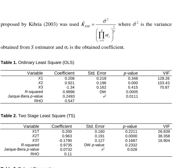
From Table 1, it can be seen that estimation based on the OLS estimator produces residuals that reveals the problem of autocorrelation (DW p-value=0.0005) and multicollinearity (VIF>10) simultaneously. The problem of multicollinearity might be the reason for the wrong sign in the value of imported raw materials. We handle the problem of autocorrelation in Table 2 by transforming the data set. The original data set is transformed using



ˆ 0.547



(from Table 1) to correct the problem of autocorrelation by applying Two Stage Least Squares. Table 2 shows that the new data set obtain through transformation suffered the problem of non-normal error term using Jarque-Bera Statistic and Table 3 also shows the presence of bad leverages using robust diagnostics which might be the reason for the non-normality of the error term. The data set still suffered the problem of multicollinearity (VIF>10) as revealed in Table 2. Due to the presence of bad leverages OLS will not correctly estimate the parameters in the model. This prompts the use of the Two Stage Robust Estimators in Table 4. LTS and S estimators perform better than other estimators when we have leverages and outliers in y axis (bad leverages) in terms of the MSE (B). But the coefficient of LTS seems to be much different from the class of other estimators. We then prefer to consider S estimator in its stead. Due to the occurrence of both problem of multicollinearity and bad leverages in the new data set, we then use the Ridge combined with S estimator adopted from the concept of Samkar and Alpu (2010) to compute the ridge parameter. Geometric version of the ridge parameter

proposed by Kibria (2003) was used 2 1 1 ˆ ˆ GM p _p i i K         





where



ˆ2 is the variance

obtained from S estimator and

α

i is the obtained coefficient.

Table 1. Ordinary Least Square (OLS)

Variable Coefficient Std. Error p-value VIF

X1 0.208 0.218 0.348 128.26 X2 0.921 0.196 0.000 103.43 X3 -1.34 0.162 0.415 70.87 R-squared 0.9896 DW 0.0005 Jarque-Bera p-value 0.2493 σ2 _0.0111 RHO 0.547

Table 2. Two Stage Least Square (TS)

Variable Coefficient Std. Error p-value VIF

X1T 0.200 0.160 0.2211 26.839 X2T 0.963 0.191 0.0000 38.358 X3T -0.1790 0.127 0.1687 16.904 R-squared 0.9735 DW p-value 0.2332 Jarque-Bera p-value 0.0732 σ2 _0.028 RHO 0.11

Table 3. Robust Diagnostics

Observation Mahalanobis Robust MCD

Distance Leverage

Standardized

Robust Residual Outlier

12 1.5024 5.8641 * 4.7737 * 14 0.9716 3.0421 4.9055 * 15 4.6559 29.4708 * 9.1178 * 16 1.0615 8.2135 * 11.2653 * 17 1.6992 8.6846 * 1.4033 18 2.2534 19.0971 * -0.5591 20 3.0865 24.3649 * -2.4415 21 3.8595 26.6181 * 0.4649 22 1.2315 8.8886 * 0.4301 30 3.421 3.0381 16.2649 * 31 1.2827 1.1007 -8.5191 *

Table 4. Two Stage Robust Estimators and OLS Variables OLS TS M MM S LTS X1T 0.208 0.200 0.329 0.328 0.346 0.032 X2T 0.921 0.963 0.976 0.976 0.963 1.723 X3T -1.34 -0.1790 -0.228 -0.228 -0.221 -0.648 R-squared 0.9896 0.9735 0.7918 0.7939 0.8023 0.9951 σ2 _{0.0111 0.028 0.0102 0.019 0.017 0.003} MSE(B) 0.1122 0.0782 0.0324 0.0303 0.0272 0.029

Table 5. Two Stage Robust Ridge Estimators

Variables Coefficient VIF

X1 0.3443 1.2972 X2 0.4278 1.0011 X3 0.1836 1.5526 MSE(β) 0.071687 K 0.097

Conclusion

OLS performs better than other estimators when there is no violation of assumptions in Classical Linear Regression Model. In this study the problem of autocorrelation was handled using Two Stage Least Square. The problem of multicollinearity and outlier are still presents. OLS will not be efficient because of the present of both problem therefore we apply Robust Methods to the transformed data. S and LTS estimators perform better than other Robust Methods in terms of the MSE. S estimator was chosen because LTS does not correctly estimate the model when compared with other estimators. Ridge parameter K is then obtained using the estimates obtain from S estimation. Robust ridge estimates was computed. Two stage robust ridge estimator performs better than the Generalized Two stage ridge regression proposed by Hussein et al (2012). This is because after the problem of autocorrelation was corrected in the study of Hussein et al (2012), the data sets still suffered the problem of multicollinearity and outlier. This was corrected in this study by obtaining the ridge parameter using a robust estimator instead of OLS.

Authors’ note

References

Askin, G. R., & Montgomery, D. C. (1980). Augmented robust estimators. Technometrics, 22(3), 333-341. doi:10.1080/00401706.1980.10486164

Ayinde, K. & Lukman, A. F. (2014). Combined estimators as alternative to multicollinearity estimation methods. International Journal of Current Research, 6(1), 4505-4510.

Barnett, V. & Lewis, T. (1994). Outliers in statistical data (Vol. 3). New York: Wiley.

Belsley, D. A., Kuh, E., & Welsch, R. E. (1980). Regression diagnostics: identifying influential data and sources of collinearity. New York: Wiley.

Chatterjee, S., Hadi, A. S. (1986). Influential observations, high leverage points, and outliers in linear regression. Statistical Science, 1(3), 379-416. doi:10.1214/ss/1177013622

Eledum, H. Y. A., Alkhalifa, A. A. (2012). Generalized two stages ridge regression estimator for multicollinearity and autocorrelated errors. Canadian Journal on Science and Engineering Mathematics, 3(3), 79-85.

Green, W.H. (1993). Econometric analysis (2nd _{ed.). New York: MacMillan.}

Gujarati, D. N. (1995). Basic econometrics (3rd _{ed.). New York:}

McGraw-Hill.

Gujarati, D. N. (2003). Basic econometrics (4th ed.) (pp. 748, 807). New Delhi: Tata McGraw-Hill.

Hawkins, D. M. (1980), Identification of Outliers, London: Chapman & Hall. Hoerl, A. E. & Kennard, R.W. (1970). Ridge regression biased estimation for nonorthognal problems. Technometrics, 12(1), 55-67.

doi:10.1080/00401706.1970.10488634

Holland, P. W. (1973). Weighted ridge regression: Combining ridge and robust regression methods (NBER Working Paper No.11). Cambridge, MA: National Bureau of Economic Research. doi:10.3386/w0011

Huber, P. J. (1964). Robust estimation of a location parameter. The Annals of Mathematical Statistics, 35(1), 73-101.doi:10.1214/aoms/1177703732

Keijan, L. (1993). A new class of biased estimate in linear regression. Communications in Statistics-Theory and Methods, 22(2), 393-402.

doi:10.1080/03610929308831027

Midi, H., & Zahari, M. (2007). A simulation study on ridge regression estimators in the presence of outliers and multicollinearity. Jurnal Teknologi, 47(C), 59-74. doi:10.11113/jt.v47.261

Rousseeuw, P.J. (1984). Least Median of Squares Regression. Journal of the American Statistical Association, 79, 871–880.

doi:10.1080/01621459.1984.10477105

Rousseeuw P. J., & Leroy A. M. (1987). Robust Regression and Outlier Detection. New York: Wiley-Interscience.

Rousseeuw, P. J. & Van Driessen, K. (1998). Computing LTS regression for large data sets. Technical Report, University of Antwerp, submitted.

Rousseeuw P. J., & Yohai, V. (1984). Robust regression by means of S-estimators. In J. Franke, W. Härdle & D. Martin (Eds.), Robust and Nonlinear Time Series Analysis (Vol. 26, pp. 256-272). New York: Springer-Verlag. doi:10.1007/978-1-4615-7821-5_15

Ryan, T.P. (1996). Modern Regression Method. Canada: John Wiley & Sons. Samkar, H. & Alpu, O. (2010). Ridge regression based on some robust estimators. Journal of Modern Applied Statistical Methods, 9(2), 17.

Yohai, V. J. (1987). High breakdown point and high breakdown-point and high efficiency robust estimates for regression. The Annals of Statistics, 15(2), 642-656. doi:10.1214/aos/1176350366