Advances in clustering based on inter-cluster mapping

Advances in Clustering based on

Inter-Cluster Mapping

A thesis submitted in fulfilment of the requirements for The degree Doctor of Philosophy

by

Arshad Muhammad Mehar

Student ID: 16684993

September 2016

Master of Information Technology (Edith Cowan University, Australia) 2001 Graduate Diploma of Science (Computer Studies) (Edith Cowan University, Australia) 1999

Bachelor of Science (Punjab University Lahore, Pakistan) 1997

School of Computing, Engineering and Mathematics

College of Health and Sciences, Western Sydney University

To the memory of my parents

ACKNOWLEDGMENT

First of all, I am deeply thankful to my supervisors, Professor Anthony Maeder and Dr. Kenan Matawie, for providing me an opportunity to study under their supervision. Their assistance, motivation and encouragement throughout the course of this work was amazing. I was very fortunate to have them and their guidance, feedback, scholarly and moral support. I will always treasure their comprehensive, broad knowledge and enthusiasm. I believe that without their care, supervision and friendship, I would not have been able to complete this work. I am most indebted to my parents Ghulam Rasool and Khursheed Bibi for their love, continuing affection, patience and constant encouragement during. May God protect them and bless them in paradise. I deeply thank my wife Sarwat Arhsad for her love and understanding, especially for her comforting me when I encountered sorrow and loneliness. I would like to express my appreciation to my children, Samia Arshad Mehar, Ismail Arshad Mehar, Yahiya Arshad Mehar and Laiba Arshad Mehar for their support during my study for this degree. Finally, my thanks also go to other faculty and staff members of the School of Computing, Engineering & Mathematics and to my fellow graduate students, for providing a friendly and enjoyable environment during my time here.

Abstract

Data mining involves searching for certain patterns and facts about the structure of data within large complex datasets. Data mining can reveal valuable and interesting relationships which can improve the operations of business, health and many other disciplines. Extraction of hidden patterns and strategic knowledge from large datasets which are stored electronically, is therefore a challenge faced by many organizations. One commonly used technique in data mining for producing useful results is cluster analysis. A basic issue in cluster analysis is deciding the optimal number of clusters for a dataset. A solution to this issue is not straightforward as this form of clustering is unsupervised learning and no clear definition of cluster quality exists. In addition, this issue will be more challenging and complicated for multi-dimensional datasets. Finding the estimated number of clusters and their quality is generally based on so-called validation indexes. A limitation with typical existing validation indexes is that they only work well with specific types of datasets compatible with their design assumptions. Also their results may be inconsistent and an algorithm may need to be run multiple times to find a best estimate of the number of clusters. Furthermore, these existing approaches may not be effective for complex problems in large datasets with varied structure. To help overcome these deficiencies, an efficient and effective approach for stable estimation of the number of clusters is essential.

Many clustering techniques including partitioning, hierarchal, grid-base and model-based clustering are available. Here we consider only the partitioning method e.g. the

k-means clustering algorithm for analysing data. This thesis will describe a new approach for stable estimation of the number of clusters, based on use of the k-means

clustering algorithm. First results obtained from the k-means clustering algorithm will be used to gain a forward and backward mapping of common elements for adjacent and non-adjacent clusters. These will be represented in the form of proportion matrices which will be used to compute combined mapped information using a matrix inner product similarity measure. This will provide indicators for the similarity of mapped elements and overlap (dissimilarity), average similarity and average overlap (average dissimilarity) between clusters. Finally, the estimated number of clusters will be decided using the maximum average similarity, minimum average overlap and coefficient of variation measure.

The new approach provides more information than an application of typical existing validation indexes. For example, the new approach offers not only the estimated number of clusters but also gives an indication of fully or partially separated clusters and defines a set of stable clusters for the estimated number of clusters. The advantage of the new approach over several existing validation indexes for evaluating clustering results is demonstrated empirically by applying it on a variety of simulated and real datasets.

Table of Contents

Chapter1 Introduction …..………1

1.1 Healthcare Datasets ... 2

1.2 Conceptual and Empirical Aspects ... 3

1.3 Contributions to Knowledge ... 4

1.4 Research Outcomes ... 5

1.5 Thesis Overview... 6

Chapter 2 Data Mining…..………7

2.1 Introduction ... 7 2.2 Supervised Learning... 9 2.2.1 Regression Analysis ... 10 2.2.1.1 Linear Regression ... 10 2.2.1.2 Multiple Regression ... 11 2.2.1.3 Logistic Regression ... 11 2.2.2 Classification ... 11

2.2.2.1 Rule Based Classifiers ... 12

2.2.2.2 Bayesian Classifiers ... 13

2.2.2.3 Decision Trees ... 14

2.2.2.4 Artificial Neural Networks ... 15

2.3 Unsupervised Learning ... 16

2.3.1 Factor Analysis ... 16

2.3.2 Principal Component Analysis ... 17

2.3.3 Association Rules ... 18

2.3.4 Cluster Analysis ... 19

2.3.4.1.1 K-Means... 20

2.3.4.1.2 K-Medoids or Partition Around Medoid (PAM) ... 21

2.3.4.1.3 CLARA (Clustering LARge Application) ... 22

2.3.4.1.4 CLARANS (CLustering Algorithm based on RANdomized Search)…... 24

2.3.4.1.5 K-Modes and K-Prototypes ... 26

2.3.4.2 Hierarchical Clustering ... 28

2.3.4.3 Density Based Clustering ... 29

2.3.4.4 Grid-Based Clustering ... 29

2.3.4.5 Model Based Clustering ... 30

2.4 Fundamental Steps in Data Preparation ... 31

2.4.1 Variable Types ... 31

2.4.2 Data Visualization ... 32

2.4.3 Data Cleansing ... 34

2.4.4 Variable Selection and Scaling ... 34

2.4.5 Measures of Similarity and Dissimilarity ... 36

2.5 Application of Data Mining in Health ... 39

2.5.1 Drug Usage... 40

2.5.2 Epidemiology ... 40

2.5.3 Hospital Utilization ... 41

2.6 Summary ... 43

Chapter 3 Clustering Evaluation…..….…….……….44

Introduction ... 44

3.1 Issues with K-Means ... 45

3.2 Cluster Quality ... 46 3.3

Evaluating Clusters ... 47

3.4 Internal Validations ... 49

3.5 3.5.1 Dunn (𝐷𝑢𝑛𝑛_{𝑖𝑛𝑑𝑒𝑥}) Index ... 50

3.5.2 Duda and Hart ((𝐷𝐻𝑖𝑛𝑑𝑒𝑥) Index ... 50

3.5.3 Calinski and Harabasz (𝐶𝐻𝑖𝑛𝑑𝑒𝑥) Index ... 51

3.5.4 Silhouette (𝑆𝑖𝑙_{𝑖𝑛𝑑𝑒𝑥}) Index ... 51

3.5.5 Davies-Bouldin(𝐷𝐵_{𝑖𝑛𝑑𝑒𝑥}) Index ... 52

3.5.6 SD (𝑆𝐷_{𝑖𝑛𝑑𝑒𝑥}) Index ... 52

3.5.7 Gap Statistics (𝐺𝑎𝑝_{𝑖𝑛𝑑𝑒𝑥}) Index ... 53

3.5.8 Cubic Clustering Criterion (𝐶𝐶𝐶𝑖𝑛𝑑𝑒𝑥) Index ... 54

Summary ... 55

3.6 Chapter 4 New Approach………..………..57

4.1 Introduction ... 57

4.2 Overview of the New Approach ... 59

4.3 Development of the Approach ... 62

4.3.1 Forward and Backward Elements Mapping ... 63

4.3.2 Combined Proportions and Combined Elements Matrices ... 68

4.3.3 Computing Cluster Similarity and Overlap (Dissimilarity) ... 73

4.3.4 Cluster Stability ... 74

4.4 Computation Illustration for the New Approach ... 77

4.4.1 Inter Cluster Mapping when 𝑘 = 2 and 𝑟 = 1 ... 77

4.4.2 Combined Mapped Proportion Matrices ... 78

4.4.3 Combined Mapped Elements Matrices ... 79

4.6 Conclusion ... 86

Chapter 5 Application to Simulated Data………….………..88

5.1 Introduction ... 88

5.2 Type1 Datasets: Spherical Clusters of Different Sizes ... 89

5.3.1 Case1: High Density Clusters ... 91

5.3.2 Case2: High-to-Medium Density Clusters ... 99

5.3.3 Case3: Medium-to-Low Density Clusters ... 103

5.3.4 Case4: Low Density Clusters ... 105

5.3 Type2 Datasets: Spherical Clusters Equal Sizes ... 109

5.3.1 Case1: High Density Clusters ... 110

5.3.2 Case2: High-to-Medium Density Clusters ... 114

5.3.3 Case3: Medium-to-Low Density Clusters ... 118

5.3.4 Case4: Low Density Clusters ... 121

5.4 Type3 Datasets: Mixture of Clusters... 125

5.4.1 Case1: Three Clusters Mixture of Spherical and Elliptical Shapes ... 125

5.4.2 Case2: Five Clusters Mixture of Spherical and Elliptical Shapes... 128

5.4.3 Case3: Seven Spherical Clusters of Different Sizes and Density ... 132

5.4.4 Case4: Nine Square Clusters of Medium Density and Equal Sizes ... 137

5.5 Summary ... 141

Chapter 6 Application to Real world Datasets………..………143

6.1 Introduction ... 143

6.2 Datasets with Known Clustering Structure ... 143

6.2.1 Dataset: Physical Education ... 144

6.3 Datasets with Unknown Clustering Structure ... 153

6.3.1 Dataset: Framingham Heart Study (FHS) ... 153

6.3.2 Dataset: Medical Expenditure Panel Survey (MEPS) ... 158

6.4 Summary ... 164

Chapter 7 Conclusions……….……….…165

7.1 Discussion ... 167

7.2 Future Research Work... 170

7.3 Summary ... 173

Appendix A ... 175

Approach Implementation Using R ... 175

List of Figures

Figure 2.1: Data Mining Process. ... 8

Figure 2.2: Basic structure and components of a decision tree. ... 14

Figure 3.1: Three clusters with initial centroids randomly selected [122]…….……46

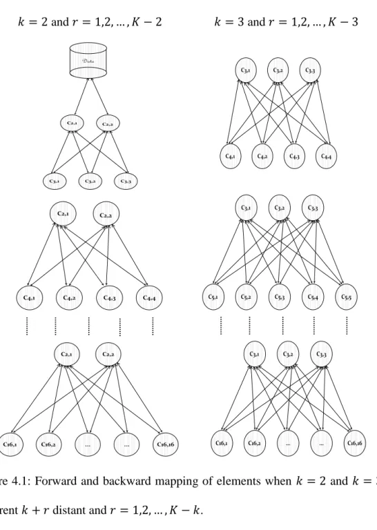
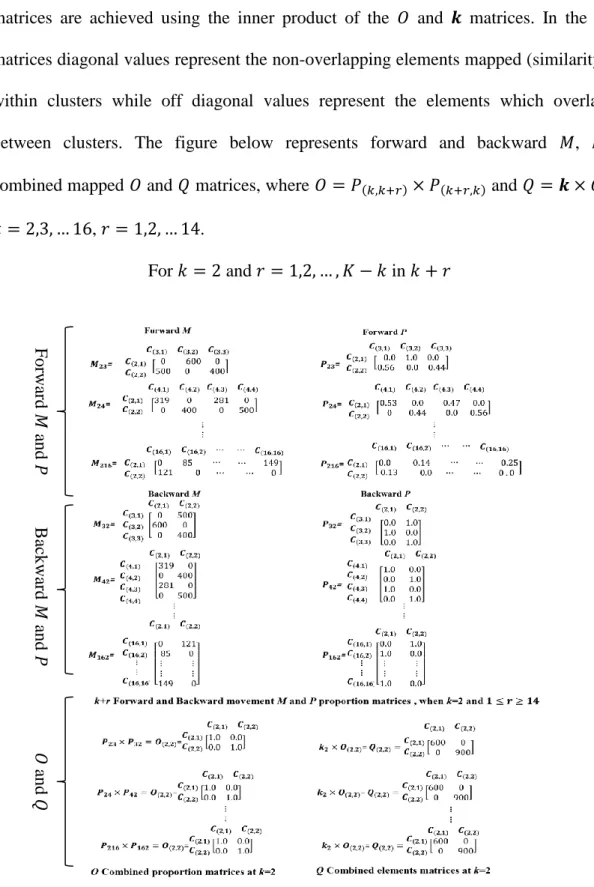
Figure 4.1: Forward and backward mapping of elements when 𝑘 = 2 and 𝑘 = 3 for different 𝑘 + 𝑟 distant and 𝑟 = 1,2, … , 𝐾 − 𝑘. ... 62

Figure 4.2: Forward and Backward mapping of common 𝑚 elements. ... 65

Figure 4.3: Forward and Backward 𝑀 matrices. ... 65

Figure 4.4: Forward and Backward proportion 𝑝 of mapped common elements. ... 67

Figure 4.5: Forward and Backward proportion 𝑃 matrices. ... 67

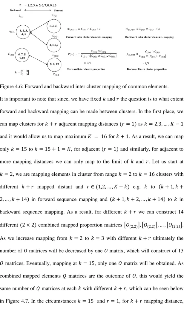
Figure 4.6: Forward and backward inter cluster mapping of common elements. ... 70

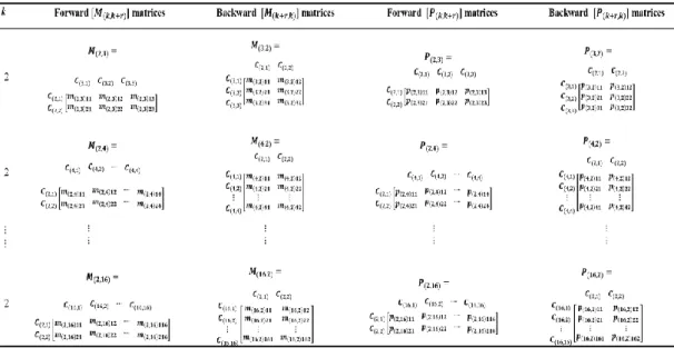
Figure 4.7: Forward and backward mapping of elements and proportion of common elements for each 𝑘 with different 𝑘 + 𝑟. ... 72

Figure 4.8: Combined mapped proportion, combined mapped elements, traces and overlap for each 𝑘 with different 𝑘 + 𝑟... 76

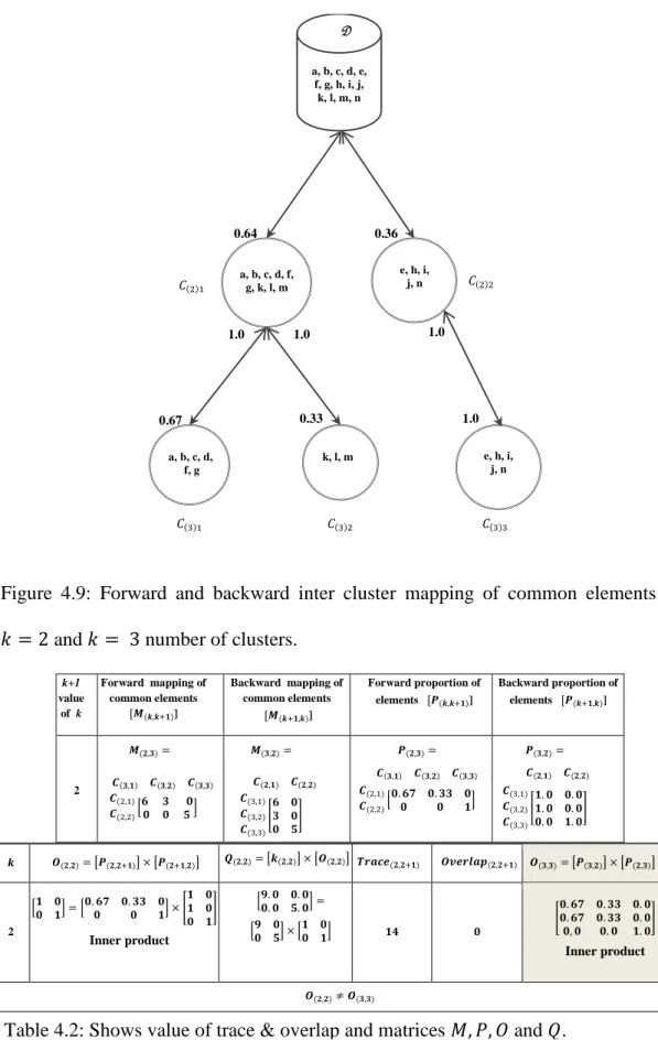
Figure 4.9: Forward and backward inter cluster mapping of common elements at 𝑘 = 2 and 𝑘 = 3 number of clusters. ... 80

Figure 4.10: Similarity at different 𝑘 with 𝑘 + 1, 𝑘 + 2 and 𝑘 + 3. ... 83

Figure 4.11: Plot (a) shows the scatter plot of the Rusipini dataset. Plot (b) shows the number of clusters obtained by a k-means algorithm using 𝑘 = 4 and membership of elements labeled with their centroids in different colours. Plots (c)-(f) show the trace values, overlap and coefficient of variation (𝐶𝑉) at different 𝑘 for 𝑘 + 𝑟 mapped distances. ... 85

Figure 5.1: Type1 dataset scatter plots for 4 cases. ... 90

Figure 5.2: Represents clusters sizes on the diagonal from 𝑘2 to 𝑘16. ... 91

Figure 5.3: Summary of elements for forward and backward mapping, proportion and combined matrices. ... 92

Figure 5.4: Forward/backward 𝑀, 𝑃 and combined mapped 𝑂, 𝑄 matrices, when 𝑘 = 3 and 𝑟 = 1,2, . . , 𝐾 − 𝑘, …, 𝑘 = 15 and 𝑟 = 𝐾 − 𝑘 = 1. ... 95

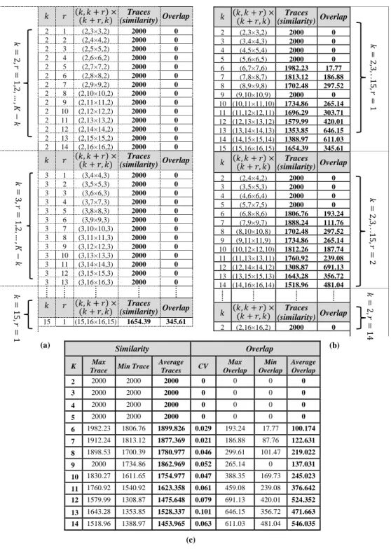
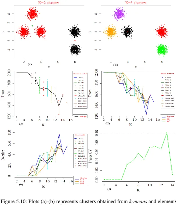
Figure 5.5: Plot (a) represents k-means clusters with elements labelled by three different colours for each cluster. Plots (b) - (d) show similarity, average similarity, average overlap and 𝐶𝑉 values respectively. ... 97 Figure 5.6: The memberships of the clusters obtained from k-means are labelled by different colours with their centroid in (a) and (b). Plots (c)-(f) show similarity, average similarity, overlap, average overlap and 𝐶𝑉 values. ... 101 Figure 5.7: The memberships of the clusters obtained from k-means are labelled by different colours with their centroid in (a) and (b). Parts (c) to (f) are plots from the values of combined 𝑄 matrices. ... 104 Figure 5.8: The membership of the clusters obtained from k-means are labelled by different colours with their centroid in (a) and (b). Plots (c) - (f) show similarity, average similarity, overlap, average overlap and 𝐶𝑉 values. ... 107 Figure 5.9: Type2 dataset scatter plots for four cases. ... 110 Figure 5.10: Plots (a)-(b) represents clusters obtained from k-means and elements are labelled in different colours for each cluster with centroids. Plots (c)-(f) show similarity, overlap, average similarity, average overlap and 𝐶𝑉. ... 112 Figure 5.11: The memberships of the clusters obtained from k-means are labelled by different colours with their centroid in (a) and (b). Plots (c)-(f) show similarity, average similarity, overlap, average overlap and 𝐶𝑉 values. ... 116 Figure 5.12: Plots (a) and (b) are the results from a k-means algorithm. Plots (c)-(f) show similarity, average similarity, overlap, average overlap and 𝐶𝑉 values. ... 120 Figure 5.13: Plots (a) and (b) show the number of clusters obtained from a k-means

clustering algorithm at 𝑘 = 2 and 𝑘 = 5. Plots (c)-(f) show values computed from 𝑄 matrices. ... 123 Figure 5.14: Plot (a) shows the scatter plot for case1 dataset while (b) shows 𝑘 = 3 clusters obtained from a k-means algorithm. Membership of different clusters is shown by different colours. Plots (c)-(f) show values computed from combined mapped elements 𝑄 matrices. ... 127

Figure 5.15: Plot (a) shows the scatter plot for case2 dataset while (b) shows the clusters obtained from a k-means algorithm and labels the membership of these clusters with different colours. Plots (c)-(f) show values computed from combined mapped elements 𝑄 matrices. ... 130 Figure 5.16: Part (a) shows scatter plot of case3 while (b) shows the number of clusters obtained from a k-means algorithm and labels the membership of clusters with different colours. Plots (c)-(f) show values computed from combined mapped elements 𝑄 matrices. ... 135 Figure 5.17: Part (a) shows the scatter plot for case4 type3 dataset while (b) shows cluster membership and centroids with different colours. Plots (c)-(f) show values computed from combined mapped elements 𝑄 matrices. ... 139 Figure 6.1: Part (a) shows the scatter plot matrix of the physical education dataset. Plot (b) shows the number of clusters obtained by a k-means algorithm using 𝑘 = 4 with membership of elements labeled in different colours. Plots (c)-(f) represent the values from Table 6.1 at different 𝑘 for 𝑘 + 𝑟 mapped distances. ... 146 Figure 6.2: Plots (a)-(d) represent the values computed from different 𝑄 matrices at different 𝑘 for 𝑘 + 𝑟 mapped distances. ... 151 Figure 6.3: Part (a) shows FHS data scatter plot matrix, (b) k-means clusters and plots (c)-(f) are values from different 𝑄 matrices at different 𝑘 for 𝑘 + 𝑟 mapped distances. ... 156 Figure 6.4: Part (a) shows a data scatter plot matrix, (b) k-means clusters when

List of Tables

Table 2.1: Computing similarity and dissimilarity metrics. ... 38 Table 4.1: Forward, backward and combined mapped proportions matrices with opposite cardinality. ... 68 Table 4.2: Shows value of trace & overlap and matrices 𝑀, 𝑃, 𝑂 and 𝑄. ... 80 Table 4.3: Summary of traces (similarity) and overlap values at different 𝑘 for 𝑘 + 1 and 𝑘 + 2 mapped distances. ... 82 Table 4.4: Summary of traces and overlap when fixed 𝑘 = 2 and 𝑘 = 3 with different 𝑘 + 𝑟. ... 84 Table 4.5: Summarises the different values of traces, overlap and 𝐶𝑉 values at different 𝑘. ... 84 Table 5.1: Type1 dataset with 3 different centroids and 4 standard deviations: (where

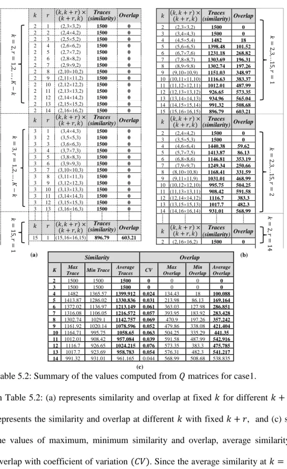
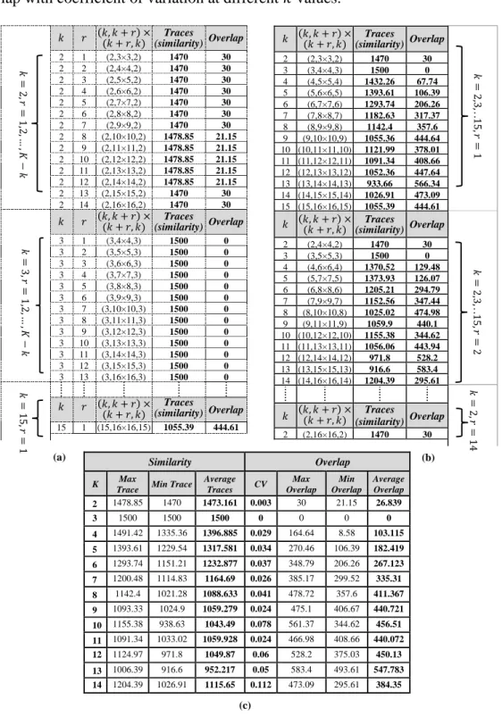
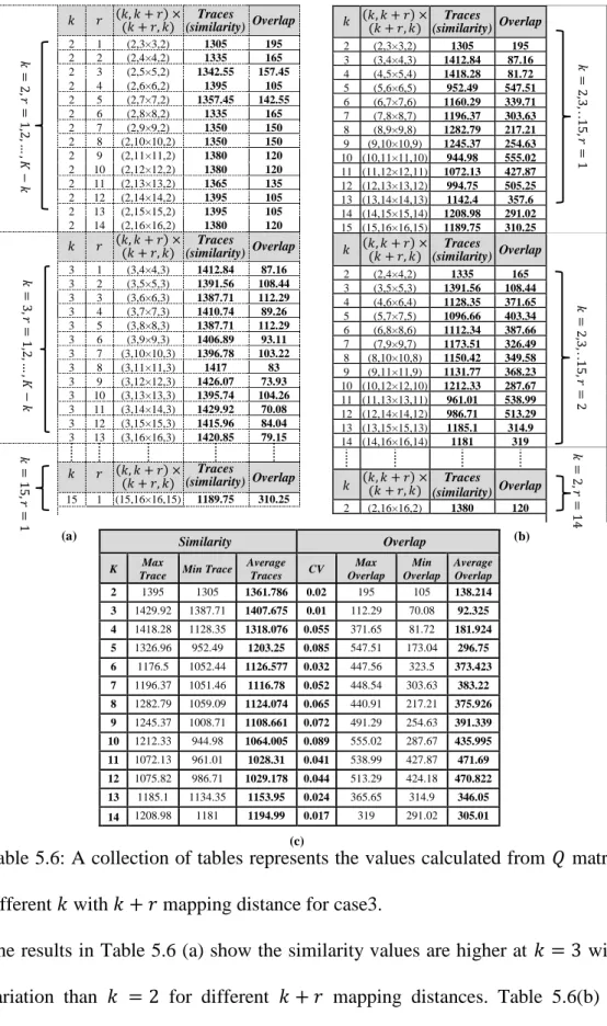
n = number of elements in each cluster, 𝜇 = mean, 𝜎 = standard deviation). ... 90 Table 5.2: Summary of the values computed from 𝑄 matrices for case1. ... 96 Table 5.3: The summary of eight different existing indexes with 5 simulated runs. The optimal number of clusters is highlighted with bold values. ... 98 Table 5.4: A collection of tables represent summary of values computed from 𝑄 matrices of case2. ... 100 Table 5.5: The summary of eight different indexes with 5 multiple runs. The optimal number of clusters is highlighted with bold values. ... 102 Table 5.6: A collection of tables represents the values calculated from 𝑄 matrices at different 𝑘 with 𝑘 + 𝑟 mapping distance for case3. ... 103 Table 5.7: The summary of values computed from the different existing indexes with optimal number of clusters is highlighted with bold values. ... 105 Table 5.8: Summary of the values computed from combined mapped elements 𝑄 matrices. ... 106 Table 5.9: The summary of values computed from the different existing indexes with the optimal number of clusters highlighted in bold. ... 108

Table 5.10: Details of Type2 datasets (where n = number of observations in each clusters, 𝜇 = mean, 𝜎 = standard deviation). ... 109 Table 5.11: A collection of tables representing the values computed from 𝑄 matrices. ... 111 Table 5.12: The summary of eight different existing indexes with 5 multiple runs. The optimal number of clusters is highlighted in bold. ... 113 Table 5.13: A collection of tables for case2 which represent the partial results computed from combined mapped elements 𝑄 matrices. ... 115 Table 5.14: The summary of eight different indexes with 5 multiple runs. The optimal number of clusters is highlighted in bold. ... 117 Table 5.15: A collection of tables summarises the values calculated from the combined elements 𝑄 matrices at different 𝑘 for 𝑘 + 𝑟 mapped distances. ... 119 Table 5.16: The summary of eight different indexes with 5 multiple runs. The optimal number of clusters is highlighted in bold. ... 121 Table 5.17: A collection of tables summarise the values calculated from 𝑄 matrices at different 𝑘 with different 𝑘 + 𝑟. ... 122 Table 5.18: The summary of eight different indexes with 5 multiple runs. The optimal number of clusters is highlighted in bold. ... 124 Table 5.19: A collection of tables show the values calculated form 𝑄 matrices at different 𝑘 with 𝑘 + 𝑟 mapping distance. ... 126 Table 5.20: Represents the optimal numbers of clusters with their values highlighted in bold from different indexes with 5 simulated runs. ... 128 Table 5.21: A collection of tables show the values calculated form 𝑄 matrices at different 𝑘 with 𝑘 + 𝑟 mapped distances. ... 129 Table 5.22: The summary of eight different indexes with 5 simulated runs. The optimal number of clusters is highlighted in bold. ... 131 Table 5.23: A collection of values calculated from 𝑄 matrices at different 𝑘 with

Table 5.24: The summary of eight different indexes with 5 multiple runs. The optimal number of clusters is highlighted in bold. ... 136 Table 5.25: Summary of the values computed form 𝑄 matrices at different 𝑘 with different 𝑘 + 𝑟 mapped distances. ... 138 Table 5.26: The summary of eight different indexes with 5 multiple runs. The optimal number of clusters is highlighted in bold. ... 140 Table 6.1: A collection of tables showing the values computed from 𝑄 matrices at different 𝑘 with different 𝑘 + 𝑟 mapping distances. ... 145 Table 6.2: Shows the optimal numbers of clusters with their values highlighted in bold from eight existing indexes with 5 multiple runs. ... 147 Table 6.3: The set of variables included in the Wisconsin Breast Cancer dataset. .. 148 Table 6.4: A collection of tables show the values calculated from 𝑄 matrices at different 𝑘 with 𝑘 + 𝑟 mapped distances. ... 150 Table 6.5: Values computed from different exisitng indexes. The optimal number of clusters is highlighted in bold. ... 152 Table 6.6: A collection of tables show the values calculated for 𝑄 matrices at different 𝑘 with 𝑘 + 𝑟 mapping distances. ... 155 Table 6.7: Framingham Heart Study values of centroid for each cluster... 157 Table 6.8: Shows the optimal numbers of clusters with their values highlighted in bold from eight different existing indexes with 5 multiple runs. ... 158 Table 6.9: A collection of tables show the values calculated from 𝑄 matrices at different 𝑘 for 𝑘 + 𝑟 mapping distances. ... 161 Table 6.10: Data clusters centroid values at 𝑘 = 4. ... 163 Table 6.11: Summarises the optimal numbers of clusters with the values highlighted in bold from eight different existing indexes with 5 multiple runs. ... 164

Chapter 1

Introduction

In the last decade an explosive growth in information technology has increased our capabilities to generate and collect data electronically. Huge resulting datasets contain a wealth of information that could be used to improve the operations and quality of many discipline studies including business and health. Therefore, knowledge discovery from databases (KDD) has become of much interest as an option for analysing these huge datasets. Originally pattern analysis and KDD were not integrated into data management systems. Consequently data mining methods have been developed to extract structure and relationships from these types of datasets independently.

A variety of data mining methods are available for KDD today, but for complex data (as in health and economics) many challenges remain to be solved for achieving greater effectiveness and better outcomes. Often these datasets are not rich in all the important fields and this makes interpretation difficult. As an example, population datasets for large complex health problems are common yet analysis of disease clusters and multidimensional patterns of socio-economic differentials in health can be difficult. Also differences in access and use of hospitals may result in adverse health outcomes and major public health issues. Gaining insights for typical clinical or population health problems such as these, with associated large complex health datasets, increasingly relies on the use of adaptive or learning methods for the analysis, rather than simple statistical processing. Some general purposes driving data mining activities in health are diagnostics, prognostics, treatment optimizations and understanding of disease mechanisms.

Although numerous generic data mining methods and algorithms have been developed, currently available methods are not designed to handle the types of complex patterns that occur in some data. In one of the most widely used data mining activities, data clustering, typically standard clustering methods (such as k-means) are used despite complications such as sparseness in the datasets. Furthermore, in these situations no satisfactory techniques have been acknowledged to find the optimal number of clusters in the datasets. The research presented here is aimed at developing and applying a new approach to address these issues.

1.1

Healthcare Datasets

Today, many healthcare organizations are engaged in the generation and accumulation of different kinds of health datasets relating to clinical practice, patient information, clinical trials, resource administration, health expenditure, policies and research. State and national health agencies in both the government and private sectors maintain extensive electronic health record systems for patients and transactional record systems for episodes of their care. Health researchers and strategists continually conduct investigations leading to the derivation of new health datasets with information which complements and extends the data associated with the above record systems. Analysing healthcare problems related to subtle and interrelated datasets such as these is difficult due to the complex structure of the datasets, and consequently developing healthcare solutions for associated problems is both challenging and demanding.

This study contributes by addressing an issue at the intersection of analysing healthcare problems and developing a new approach for evaluating the clustering results to estimate the best number of clusters. Traditionally, statistical methods are used to obtain operational information from the data while data mining methods offer

the opportunity to derive knowledge in an exploratory manner in terms of correlations, predictions, classifications, clustering and association rules. Such inductively derived healthcare knowledge can not only provide strategic insights into the practical delivery of healthcare, but also significantly impact other areas of health care systems. For example, adverse reactions to some medical pharmaceuticals are one of the leading causes of hospitalization and death [1-2]. Data mining techniques can complement existing systems for reporting spontaneous adverse drug reactions, by determining dependencies on variables such as underlying patient characteristics that are not captured in the normal drug reporting process.

1.2

Conceptual and Empirical Aspects

Many businesses and industries collect large volumes of data electronically, which are useful in determining trends in behaviour and broad pattern relationships, such as correlations and associations among different fields. Using a simple clustering approach may not reveal useful knowledge implicit within these kinds of large complex datasets. In this research, a concept of forward and backward mapping of common elements in a sequence of clustering results, with adjacent and non-adjacent clusters, is defined. There has been no such previous research found which is based on combined (forward and backward) consideration of different k-means clustering results. The word “combined” here means to map the resultant 𝑘 number of clusters with 𝑘 to 𝑘 + 𝑟 (forward) and 𝑘 + 𝑟 to 𝑘 (backward) clusters (𝑟 ≥ 1) together to define a combined set of clusters, with more information, using inner product similarity measures.

This new approach will allow us to attack complex problems in large datasets with greater confidence of achieving useful results. Efficient exploitation of the new approach in a variety of simulated and real datasets will demonstrate how it can solve

data mining problems faced today by researchers. This study will examine the use of clustering on the datasets by using the new approach and the empirical results will be compared with the performance of different existing cluster validation indexes.

1.3

Contributions to Knowledge

The main contribution of this thesis is the construction of an approach by using the standard form of k-means clustering algorithm to solve problems where the dataset is large and complex, and typically sparse in a number of relevant fields for the problem. This is achieved by defining a new forward and backward combined approach to determine the best choice of k in application of the k-means algorithm, and demonstrated across a range of simulated and real world health data problems in the domain of population health.

The research has resulted in the following specific significant contributions in analysing sequences of clusters for successive 𝑘 values, making use of the approach:

 To determine the best value of 𝑘 clusters

 To determine the stability between clusters at the best 𝑘

 To quantify properties of separation between clusters

 To determine the amount of overlapping of data element membership between clusters.

These contributions will help to answer the following major research questions:

 How can different choices of parameters and variables for a k-means clustering algorithm be combined to obtain more knowledge and explanation?

 How can different clustering results at adjacent and non-adjacent choice of 𝑘, number of clusters, be combined to form and obtain better clustering results and determining the best number of k ?

1.4

Research Outcomes

The research has produced the following outcomes:

1. A development of a mathematical formulation and computational implementation for forward and backward mapping of adjacent and non-adjacent clusters to realise the approach

2. Evidence of the effectiveness of the approach by applying it to different simulated and real datasets of different types

3. Analysis of some population health datasets by applying the approach, undertaken using R

4. Publications in conference proceedings and a book chapter related to the project.

The following three publications are the results of the contents of this research.

 Matawie, K., Mehar Muhammad, A. and Maeder, A. (2015). An approach to determine clusters overlap for k-means clustering. International Workshop on Statistical Modelling, Linz, Austria, vol 2, pp. 163-166.

 Mehar Muhammad, A., Matawie, K. and Maeder, A. (2013). Determining an Optimal Value of K in K-means Clustering. IEEE International Conference on Bioinformatics and Biomedicine (BIBM), Shanghai, China, pp. 51-55.

 Mehar, A., Maeder, A., Matawie, K. and Ginige, A. (2010). Blended Clustering for Health Data Mining. Takeda, H.(ed.) E-Health, Springer Berlin Heidelberg, 978-3-642-15515-5, pp. 130-137.

1.5

Thesis Overview

The thesis is organized into six main areas as follows.

Chapter 2 (Data Mining) will include literature review on different kinds of data mining techniques especially for clustering, describing the fundamental steps and giving examples of its application in the real world in different industries.

Chapter 3 (Clustering Evaluation) will discuss different commonly used validation indexes for evaluating clustering to determine the best number of clusters.

Chapter 4 (New Approach) will define and develop the new approach, using forward and backward mapping of common elements to the corresponding clusters and combining the mapped results.

Chapter 5 (Application to Simulated Data) will discuss the generating of extensive numbers of simulated results with different levels of variation in cluster structure, as well as discussion of a collection of datasets from the literature with varying structures, using k-means clustering and comparing the new approach with the performance of eight existing validation indexes.

Chapter 6 (Application to Real World Datasets) will examine the effectiveness of the approach and compare this with other indexes, when applied on some real datasets from UCI and elsewhere for which results are expected based on prior clustering structure. The new approach will also use datasets from medical domain where no prior clustering information are available.

Chapter 7 (Conclusion) will summarise the work and discuss scope for improvements and better outcomes with the new approach.

Chapter 2

Data Mining

This chapter will provide a literature review and brief explanation of various types of data mining techniques including supervised and unsupervised learning approaches. It will also explain the necessary steps such as data preparation, cleansing, data types, visualization, variables selection and similarity/dissimilarity measures, to understand the description and characteristics of datasets. Also, application of different data mining methods especially the clustering approach for health datasets will be discussed.

2.1

Introduction

The systematic and progressive uptake of information and communication technologies (ICT) in a variety of fields (e.g. science, economics, engineering, business and health) has led to a rapid increase in the volume of data routinely being stored in electronic form. This makes it possible to carry out large scale studies to determine the underlying structure in the large datasets from these different fields. Different types of studies for investigating potential structure are commonly based on data mining. Thus, before describing these techniques, an explanation will first be given for the overall concept of data mining. The term data mining originated from statistics, computer science and related areas and is typically used in the context of large datasets [3]. It is a newer generation approach to data analysis by data scientists, which has grown rapidly out of the need to derive useful knowledge from massive amounts of high dimensional and large volume datasets. It is based on a paradigm of exploration and confirmation - “exploratory not analytic” [4] - also known as knowledge discovery [5], by analysing data from different perspectives

and summarizing it into useful information. Technically, it is the process of finding correlations or patterns among dozens of fields [6-8] in large databases, using methods for searching through the data for patterns. Data mining can lead to the extraction of hidden predictive information from large databases which can help companies and organizations to focus on the most important information in their data warehouses [9, 10]. It is heavily used in numerous fields like banking, insurance and marketing etc. The basic steps involved in the conventional data mining process according to Fayyad [11] are shown in the figure below:

Figure 2.1: Data Mining Process.

It is important to first mention the related knowledge and understand the data mining methods and the datasets domains before we apply and progress with clustering. The basic steps for the data mining process to find and interpret patterns are summarized as follows:

 Create target data: for analysis select the appropriate data from the databases.

 Data cleaning and pre-processing: the process of cleansing data such as correcting data entry errors and deciding if outliers need removing.

Data Target Data Selection Knowledge Transformed Data Patterns Data Mining Interpretation Pre-processing Pre-processed Data ---- ---- Transformation

 Data reduction and projection: the process of finding useful features to represent the data, using dimension reduction or transformation techniques to reduce number of variables considered.

 Choosing data mining methods: the process of selecting an appropriate data mining method in order to discover patterns of interest.

 Exploratory analysis, model and hypothesis selection: the process of deciding an appropriate model, algorithm and parameters.

 Interpretation: the process of providing information or knowledge discovered about the pattern.

 Using discovered knowledge: reporting and documenting the knowledge to the interested people and also checking and comparing with previously obtained knowledge.

Data mining techniques have been categorized into two different approaches: supervised or directed learning, and unsupervised or undirected learning. The supervised approach is used for hypothesis testing or verification while unsupervised data mining is used for knowledge discovery [12]. Association rules, clustering and feature extraction are examples of unsupervised learning. Classification, estimation, and prediction are examples of supervised learning. These two approaches are described below. Use of related techniques for health datasets are discussed later.

2.2

Supervised Learning

The supervised learning approach has already pre-defined labels (classes) for information and some prior knowledge involving predictor and response variables. The predictor is also known as the descriptor or independent variable, which is used to build the model, while the response is referred to as the dependent or outcome variable, which is predicted using a predictive model [13, 14]. The supervised

learning is based on the use of a training dataset from a data source and associated response variables with already correct labels assigned [13, 15]. The several types of supervised learning techniques are regression analysis (linear, multiple, logistic) decision tree, classifier (rule base and naive base), artificial neural network and factor analysis, which will be described in more detail in the following sections.

2.2.1 Regression Analysis

Regression modelling in data mining is a method to find the relationship between dependent and independent (predictors) variables to build a model which can be used to make predictions. There are different types of well-known regression analysis techniques available which are commonly used including: linear regression, multiple regression and logistic regression which are described below.

2.2.1.1 Linear Regression

Primarily linear regression is used to predict the relationship between a single continuous predictor variable and a single continuous response variable [16]. It is a technique to produce a straight line function between independent (𝑥) variable and dependent (𝑦) variable. The mathematical form of linear regression and least squares [13, 16] are as follows:

𝑦 = 𝑎 + 𝑏𝑥 + 𝑒 (2.1)

This equation shows the expected value of (𝑦) is given by intercept (𝑎) plus (𝑥) multiplied by slope (𝑏) and includes a (𝑒) residual error.

Using least squares theory

𝑏 =∑ (𝑥𝑖− 𝑥̅)(𝑦𝑖 − 𝑦̅) 𝑛 𝑖=1 ∑𝑛 (𝑥_𝑖− 𝑥̅)2 𝑖=1 (2.2)

2.2.1.2 Multiple Regression

Datasets in many applications have hundreds or thousands of variables, many of which may have linear relationships with the response (target) variable. The main purpose of multiple regression is to provide a relationship between several independent or predictor variables and a dependent or criterion variable [16]. It is an extension of linear regression: if there are 𝑛 independent (𝑥) variables then the mathematical representation of multiple regressions [16] is

𝑦 = 𝑏0+ 𝑏1𝑥1+ 𝑏2𝑥2+ ⋯ + 𝑏𝑛𝑥𝑛 + 𝑒 (2.3)

where 𝑥₁, 𝑥₂, … , 𝑥_𝑛 are independent variables and 𝑦 is the response variable.

𝑏0, 𝑏1, 𝑏2, … , 𝑏𝑛are regression coefficients and a (𝑒) residual error.

2.2.1.3 Logistic Regression

Linear regression is only appropriate when the response variable is continuous, so it is not useful for categorical response variables. Logistic regression is used for describing the relationship between a categorical response and a set of predictor variables [14, 16]. The logistic regression has mathematical [14] form as below:

𝑃(𝑦 = 1) = 1

1 + 𝑒−(𝑏0+𝑏1𝑥1+𝑏2𝑥2+⋯+𝑏𝑘𝑥𝑘) (2.4)

2.2.2 Classification

In data mining, classification is used for predicting or assigning data points (often called objects) to one of several predefined categories [17]. Classification uses both categorical or a mixture of continuous numeric and categorical data. The difference between classification and regression is that the response is a categorical variable for classification while the response is a continuous variable for regression. It is the process of learning a target function 𝑓 which maps each attribute set

𝑋

𝑌

variety of data to provide more information in detail than a regression model [19]. There are different types of classification like rule based classifiers, Bayesian classifiers, decision tree and artificial neural network, explained further below.

2.2.2.1 Rule Based Classifiers

Rule based classifiers are used to provide knowledge in terms of a set of rules, which tell us what should be concluded in different situations. According to [20] it is a technique for classification which is collection of a set of IF-THEN rules. An IF

-THEN rule is represented in the form of “IF condition THEN conclusion”. The rules for the model are represented in a disjunctive normal form

𝑅 = 𝑟1𝑣 𝑟2𝑣 … 𝑟𝑘 (2.5)

where 𝑅 is known as the set of rules and 𝑟𝑖 ‘s are the component classification rules and 𝑣 is the “OR” operation.

For example in medical domain, the medical decision making rules are mainly designed by medical professionals rather than by algorithms [21]. A particular example is the patient’s risk of heart failure which is defined and determined by the following set of rules;

Rule 1: IF blood pressure is likely to be high

THEN risk of heart failure is high Rule 2: IF blood pressure is likely to be low

THEN risk of heart failure is low Rule 3: IF alcohol consumption is high

AND patient salt intake is high

THEN blood pressure is likely to be high Rule 4: IF alcohol consumption is low

THEN blood pressure is likely to be low Rule 5: IF units of alcohol per week are > 30

THEN alcohol consumption is high Rule 6: IF units of alcohol per week are < 20

THEN alcohol consumption is low

Rule 7: IF units of alcohol per week are >= 20 AND <= 30

THEN alcohol consumption is average

2.2.2.2 Bayesian Classifiers

Naïve Bayes Classifiers are based on Bayes Theorem which enables statistical classification for combining prior knowledge from classes with new evidence gathered from data [20]. Bayes Theorem is a statistical measure to compute conditional posterior probability from evidence of an event to understand other events [22]. According to Myatt and Johnson [14] Bayes theorem is used to compute probabilities of class membership, given specific evidence. Statistical methods are widely used for classification but success of using such methods depends on the both the size of datasets and on previous knowledge about the dataset. If 𝐴 and 𝐵 are random variables then the conditional and joint probability of 𝐴 and 𝐵 be used in the mathematical representation as described by Larose [16] as follows:

𝑃(𝐴 𝐵⁄ ) =𝑃(𝐴 ∩ 𝐵) 𝑃(𝐵) (2.6) =𝑁𝑢𝑚𝑏𝑒𝑟 𝑜𝑓 𝑜𝑢𝑡𝑐𝑜𝑚𝑒 𝑖𝑛 𝑏𝑜𝑡ℎ 𝐴 𝑎𝑛𝑑 𝐵 𝑛𝑢𝑚𝑏𝑒𝑟 𝑜𝑓 𝑜𝑢𝑡𝑐𝑜𝑚𝑒𝑠 𝑖𝑛 𝐵 𝑃(𝐴 ∩ 𝐵) = 𝑃(𝐴 𝐵⁄ ) ∗ 𝑃(𝐵) (2.7) 𝑃(𝐴, 𝐵) = 𝑃(𝐴 𝐵⁄ ) ∗ 𝑃(𝐵) = 𝑃(𝐵 𝐴⁄ ) ∗ 𝑃(𝐴) (2.8) Also, 𝑃(𝐵 𝐴⁄ ) =𝑃(𝐴 ∩ 𝐵) 𝑃(𝐴) (2.9)

𝑃(𝐴 ∩ 𝐵) = 𝑃(𝐵 𝐴⁄ ) ∗ 𝑃(𝐴) (2.10)

𝑃(𝐴 𝐵⁄ ) ∗ 𝑃(𝐵) = 𝑃(𝐵 𝐴⁄ ) ∗ 𝑃(𝐴) (2.11)

By rearranging the above equations the following formula is obtained which is known as Bayes Theorem:

𝑃(𝐴 𝐵⁄ ) = 𝑃(𝐵 𝐴⁄ ) ∗ 𝑃(𝐴)

𝑃(𝐵) (2.12)

2.2.2.3 Decision Trees

A decision tree is a collection of decision nodes which are connected by branches, moving downward from the root node (decision of choice) through a path of interval nodes and finishing in leaf nodes [23].

Root node: The top level node is called root node or parent node. It consists of zero or more outgoing edges but no incoming edges.

Internal node: It is also known as non-leaf node which has only one incoming edge and two or more than two outgoing edges.

Leaf or terminal node: It is also known as external node which has zero child nodes and only one incoming edge but no outgoing edges.

Figure 2.2: Basic structure and components of a decision tree. Disease 𝐴 Medication 1 𝑥 Medication 2 𝑦 Success Success Failure Failure

2.2.2.4 Artificial Neural Networks

The study of artificial neural networks (ANN) was inspired by biological thinking systems such as how brains process information [23]. An artificial neural network is a computational and mathematical model based on biological neural networks. It was originally developed by neurobiologists and psychologists who sought to develop and test computational analogues of neurons, using a set of connected input/output units where each connection has a weight associated with it [20]. Artificial neural networks are used in data mining tasks to build nonlinear predictive models that learn through training [24]. According to [25] the simplest form of ANN is the perceptron which is a linear combination of the measurements in 𝑥 that is represented by the equation:

𝑓(𝑥) = ∑ 𝑤_𝑖𝑥_𝑖

𝑝

𝑖=1

(2.13) where 𝑤_𝑖 , 1 ≤ 𝑖 ≤ 𝑝 are the weight parameters of the model.

The most common form of ANN is the multilayered perceptron (MLP) which uses neurons arranged as layers (input, hidden and output layers) [26].

𝑦 = 𝑓 (∑ (𝑣𝑗 ∗ 𝑓 (∑ 𝑤𝑖𝑗 ∗ 𝑥𝑖 𝑝 𝑖=0 )) 𝑛 𝑗=1 ) (2.14)

In neural networks Larose [16], the input layers uses the input values from the training dataset along with the target set of variables and the output layers to compute the output value. Then the error is the difference between the output value and the actual value, by which the sum of squared errors can be computed. There are many different types of artificial neural networks and neural network algorithms but the most famous neural network algorithm is back-propagation. The algorithm in this approach has two phases, the forward phase and the backward phase, to compute the

error of an output node. In the forward phase weights are computed in the forward direction from the weights obtained in the previous iteration, to affect the output value of every neuron in the network. So the outputs of neurons at position 𝑥 are calculated prior to calculating the outputs at position 𝑥 + 1. In the backward direction the updated weight formula is applied in reverse that is weights at position

𝑥 + 1 are updated before the weights at position 𝑥 are updated. The weights in the back-propagation are proportionally decreased or increased depending upon the direction (either forward or backward) of the error as it works its way through the system of nodes. Once all the weights have been recomputed, the input for another case is entered into the network and this process is repeated exhaustively to make the best prediction through all of the input data patterns during the training phase [18, 27].

2.3

Unsupervised Learning

In data mining unsupervised learning has no pre-defined labels (classes) and is similar to exploratory data analysis which aims to find the hidden information and relations among the variables. This approach has no target (predictor) and response variables to determine the prediction values [13]. It includes factor analysis, principal components, association rules, cluster analysis. In this section these will be described below.

2.3.1 Factor Analysis

Factor analysis is a generic term for the family of multivariate statistical techniques for the reduction of a set of observable variables into a much smaller number of latent factors. The primary purpose of factor analysis is data reduction and summarization [28]. It is used to find a set of hidden factors or latent attributes from the original set of variables, often as a linear combination [18]. This technique was

originally developed to investigate human intelligence [28] for exploring the relations among observed data to assess underlying factors that may not be observed directly [29]. A mechanism and mathematical model for determining a set of hidden factors [26] by performing linear transformations on observed variables, 𝑥₁, 𝑥₂, … , 𝑥_𝑝 to determine the set of factors 𝑓1, 𝑓2, … , 𝑓𝑝, such that

{ 𝑥₁− 𝜇₁ = 𝑙₁₁𝑓₁+ 𝑙₁₂𝑓₂+ ⋯ + 𝑙_1𝑚𝑓_𝑚+ 𝜀₁ 𝑥2− 𝜇2 = 𝑙21𝑓1+ 𝑙22𝑓2 + ⋯ + 𝑙2𝑚𝑓𝑚+ 𝜀2 ⋮ ⋮ ⋮ ⋮ ⋮ 𝑥𝑝− 𝜇𝑝 = 𝑙𝑝1𝑓1+ 𝑙𝑝2𝑓2+ ⋯ + 𝑙𝑝𝑚𝑓𝑚+ 𝜀𝑝 (2.15)

where, 𝜇₁, 𝜇₂, … , 𝜇_𝑝 are the means of the variables 𝑥₁, 𝑥₂, … , 𝑥_𝑝 and the terms

𝜀₁, 𝜀₂, … , 𝜀_𝑝 represent the unobservable part of variables 𝑥₁, 𝑥₂, … , 𝑥_𝑝 which are also called specificfactors. The terms 𝑙_𝑖𝑗, 𝑖 = 1,2, … , 𝑝 and 𝑗 = 1,2, … , 𝑚 are known as the loadings. The factors 𝑓1, 𝑓2, … , 𝑓𝑚 are known as the common factors. This can be written in matrix form as follows:

𝑋 − 𝜇 = 𝐿𝐹 + 𝜀 (2.16)

Given the observed variables 𝑋, along with their means 𝜇, we attempt to find the set of factors 𝐹 and the associated loadings.

2.3.2 Principal Component Analysis

Principal component analysis (PCA) is a standard tool in modern data analysis which was introduced for data reduction or dimension reduction for multidimensional data [28]. It is a technique to find a new set of dimensions that represents the variability of the new data in better way [18]. The basic idea of principal component analysis is to determine a set of linear transformations of a large number of correlated variables such that the new set of variables could provide most of the variance in a relatively smaller number of uncorrelated variables [30]. The mathematical formulations for PCA in [26] is described as; suppose if 𝑥₁, 𝑥₂, … , 𝑥_𝑝 is a set of 𝑝 variables and there

are 𝑁 observations of these variables, then the mean vector 𝜇 is the vector whose

𝑝 components are defined as:

𝜇_𝑖 = 1 𝑁∑ 𝑥𝑖𝑗

𝑁 𝑗=1

, 𝑖 = 1,2, … , 𝑝 (2.17)

The unbiased 𝑝 × 𝑝 variance–covariance matrix of this sample is defined as

𝑆 = 1 𝑁 − 1∑(𝑥𝑗 − 𝜇)(𝑥𝑗 − 𝜇) ′ 𝑁 𝑗=1 (2.18) Finally, the 𝑝 × 𝑝 correlation matrix 𝑅 of this sample is defined as

𝑅 = 𝐷−12𝑆𝐷12 (2.19)

where the matrix 𝐷

1

2 _{is the sample standard deviation matrix, which is calculated}

from the covariance 𝑆 as the square root of its diagonal elements, while the matrix

𝐷−12 _{is the inverse of} 𝐷 1 2 𝐷12 = [ √𝑆11 0 ⋯ 0 0 √𝑆22 ⋯ 0 ⋮ ⋮ ⋱ ⋮ 0 0 ⋯ √𝑆𝑝𝑝_] (2.20) 2.3.3 Association Rules

In data mining, use of association rules is an unsupervised learning process where no a priori information being used. It is a process for determining important relationships between variables, which is also known as affinity analysis or basket analysis [31-33]. Each association rule is in the form of “if antecedent, then consequent” together with a degree of the support and confidence associated with each of the rules [23, 34]. These two terms, support and confidence, are very important in measuring the strength of the association (relationship) rule for the products or items. To measure the association rules two terms need to be define,

support in which we determine how often a rule is applicable in the given dataset while confidence determines how frequent items 𝐼 appeared in transactions 𝑇 found to be true [35-37]. In [32] association rules are explained such as, suppose 𝐼 =

𝐼1, 𝐼2, … , 𝐼𝑚 are set of various items and 𝑇 = 𝑇1, 𝑇2, … , 𝑇𝑛 are transactions in such a way that any transaction is a subset of items taken from 𝐼 i.e. 𝑇 ⊆ 𝐼. Then an association rule is an implication of the form 𝐴 ⟹ 𝐵 where, 𝐴 and 𝐵 are a disjoint set of items i.e. 𝐴 ∩ 𝐵 = ∅ where 𝐴 is known as antecedent and 𝐵 consequent. In [38] a study was carried out to describe association rules for both categorical and quantitative variables for large data. One of the most popular a priori rules, which allows that any subset of frequent items must be frequent is known as “co-occur”. Most of the forms of association rule algorithms such as Apriori, Charm, FP-growth, Partition and DIC and MagnumOpus [39] are based on this.

2.3.4 Cluster Analysis

Cluster analysis is the process of grouping a set of data values (often called objects) into classes of similar objects. It results in groups of data objects that are similar to one another within the same cluster and are dissimilar to the objects in other clusters [20]. There is a wide variety of clustering algorithms and the behaviour of every algorithm is different. Some algorithms may produce different results on the same dataset on different occasions, while different algorithms may lead to different results on the same dataset. Cluster analysis has been utilized successfully in various types of fields and problems: for example, in medicine, clustering cures for diseases, or symptoms of diseases can lead to very useful deductions of relatedness; in psychiatry a better way of therapy may be based on clustering symptoms such as paranoia, schizophrenia, etc. and in archeology clustering may establish taxonomies of stone tools, funeral objects, etc. [40, 41]. There are various types of cluster

techniques that are divided into different categories such as partitioning, hierarchical, density based and model based methods, discussed in the sections below.

2.3.4.1 Partitioning Methods

In cluster analysis, partitioning algorithms divide the dataset into clusters based on some criterion applied to simple cluster statistics, such as means, modes and medoids. This is a very simple, basic and iterative approach to determine clusters, which partition the 𝑁 number of objects in the D dataset into 𝑘 number of clusters with (𝑘 ≤ 𝑁). In this section some well-known partitioning clustering algorithms ( k-means, k-medoids (PAM), k-modes, CLARA and CLARANS) are described below:

2.3.4.1.1 K-Means

k-means clustering is a technique that classifies a given set of data into clusters, which are represented by their centroids in such a way that objects within a group are more similar to each other than objects in different groups [42] and this is regarded as one of the simplest clustering techniques [43]. In the k-means method as described by Han and Kamber [20], 𝑁 number of objects are partitioned into

𝑘 number of clusters starting with 𝑘 initial centroid guesses, where 𝑘 is the number of desired clusters specified by the user. Each point is assigned to the closest centroid and each collection of points assigned to a centroid defines a cluster. For each cluster the centroid is updated based on the points assigned to the cluster, and then the algorithm repeats the assigning and update process until no point changes between clusters and consequently all centroids remain the same. The steps in the k-means

algorithm are as follows: Input:

k : The number of clusters, D : Dataset containing N objects.

Output:

A set of 𝑘 clusters. Method:

1) Arbitrarily choose k objects from D as the initial cluster centers. 2) Repeat

3) Reassign each object to the cluster to which the object is the most similar, based on the mean value of the objects in the cluster;

4) Update the cluster means, i.e., calculate the mean value of the reassigned objects for each cluster;

5) Until no change;

k-means is more efficient and effective for dealing with large datasets than some other clustering algorithms, and its overall computational complexity is 𝑂(𝑁𝑘𝑡), where 𝑁 = number of objects in the dataset, 𝑘 = number of clusters and 𝑡 = number of iterations. It is not appropriate for determining clusters with non-convex shapes and clusters of very different size. It is also sensitive to noise and outlier objects which may impact the convergence of the mean values.

2.3.4.1.2 K-Medoids or Partition Around Medoid (PAM)

k-medoids clustering is also a partitioning based clustering algorithm: it is a modified form of k-means that partitions the data based on medoids. It is also known as PAM (partition around medoids) described in [44] and its process is closely related to k-means. A problem in k-means clustering is that it is very sensitive to the outliers and there may be no objects close to the mean (or centroid) in the clusters [45]. Due to this issue the medoid object is chosen from the data to represent the cluster, which is a better choice than the centroid as it is still a central object in the cluster but is less sensitive to others.

The steps in the k-medoids algorithm are as follows: Input:

𝑘: The number of clusters, D : Data set containing 𝑁objects. Output:

A set of 𝑘 clusters. Method:

1) Choose 𝑘 objects from D reprehensive objects as the initial medoids. 2) Repeat

3) Reassign each object to the cluster with nearest object.

4) For each representative object randomly select a non-representative object. 5) Compute the total dissimilarity cost by swapping representative object with

randomly non-representative object.

6) If total cost < 0 then replace representative object with non-representative object.

7) Until no change.

Experimental results using the PAM algorithm showed satisfactory performance for small datasets (e.g., 100 objects in 5 clusters) [44], while k-medoids was costly and inefficient for large datasets [46]. The computation complexity for each iteration is

𝑂(𝑘(𝑁 − 𝑘)2_{) and for large values of 𝑁 and 𝑘 computation will be much more} expensive than k-means.

2.3.4.1.3 CLARA (Clustering LARge Application)

CLARA clustering is designed and proposed by Kaufman and Rousseeuw [44] for partitioning larger datasets than would be desirable when using PAM, and is based on sampling. In this approach, instead of finding representative objects as medoids

for the whole dataset, it draws a random sample of objects from the dataset and then applies PAM on this sample to find the candidate medoids. If the sample is drawn in a sufficiently random way the sample medoids will represent the entire dataset well enough. For a better approximation CLARA draws multiple random samples and applies the PAM to each sample to find the best clustering partitions as output. The clustering measure can be based on the average dissimilarity of the objects for the entire dataset and not only for those objects in the random samples. The steps in the CLARA algorithm are as follows:

Input:

𝑘: The number of clusters, D : Data set containing 𝑁objects. Output:

A set of 𝑘 clusters. Method:

1) For 𝑖 = 1 to 5 , repeat the following steps:

2) Draw a sample of 40+2𝑘 objects randomly from the entire dataset, apply PAM algorithm to find the medoids of the sample.

3) For each object in the entire dataset, determine which of the 𝑘 medoids is the most similar to object.

4) Calculate the average dissimilarity of clustering obtained in the previous step. If this value is less than the current minimum, use this value and retain the 𝑘 medoids found in step (2) as the best medoids obtained so far.

5) Return to step (1) to start next iteration.

Experiments results reported in [44] show that five samples of size 40 +2𝑘 give satisfactory results in a dataset of size 1000 observations in 10 clusters. However, as

CLARA is based on sampling to find the best 𝑘 medoids it will not necessarily find the best clustering, and if the random sampling is biased it will degrade clustering results for the whole dataset using this approach. In [47] the proposed solution to handle this problem is to draw several samples and use these to cluster the entire dataset several times, and finally select the results with minimum average dissimilarity. The computational complexity for each iteration is 𝑂(𝑘𝑠2 + 𝑘(𝑁 −

𝑘)), where 𝑠 = size of sample, 𝑘 = number of clusters and 𝑁 = number of objects.

2.3.4.1.4 CLARANS (CLustering Algorithm based on RANdomized Search)

CLARANS is an efficient medoids based clustering algorithm. It is used for spatial data mining to find the interesting relationships and characteristics which may be exist implicitly in large and spatial datasets. It is a combination of PAM and CLARA, but the key difference between PAM and CLARANS is that the former only searches a subset of neighbours node i.e., a set of 𝑘 mediods (set of objects) to define the cluster [48]. It is an optimization algorithm which draws a random sample of arbitrary node to check and find the maximum number of neighbours of node (maxneighbour), where random sample node is specified by the user. Here, the clustering process implies every node is a potential solution. The clustering obtained after replacing a medoid is called the neighbour of the current clustering (current node). Once a better neighbour is located with lower error, CLARANS moves to the neighbour’s node and starts the process again. If a better neighbour is not located current clustering provides (numlocal) a local minimum and the algorithm begins with newly selected nodes searching for a new local minimum. Once a user specified numbers of local minima are searched, the algorithm stops and outputs the best local minimum with lowest error (mincost).

The steps in the CLARANS algorithm are as follows: Input:

𝑘: The number of clusters, D : Data set containing 𝑁objects. Output:

A set of 𝑘 clusters. Method:

1) Input parameters maxneighbour, mumlocal. Initialize 𝑖 to 1 and mincost to a large number.

2) Set current to arbitrary node. 3) Set 𝑗 to 1.

4) Consider a random neighbour 𝑆 of current, and calculate the cost differential of the two nodes.

5) If 𝑆 has a lower cost, set current to 𝑆 and go to step 3. Otherwise increment

𝑗 by 1. If 𝑗 ≤ maxneighbour go to step 4.

6) When 𝑗 > maxneibhbour, compare the cost of current with mincost. If the former is less than mincost, set mincost to cost of current and best node to current.

7) Increment 𝑖 by one. If 𝑖 > numlocal, ouput best node and stop, otherwise, go to Step 2.

The performance of this approach is more efficient, effective and scalable than PAM and CLARA in terms of quality of clustering and running time with computational complexity 𝑂(𝑁2) [20, 49, 50] for each iteration where as above 𝑁 is the number of objects.

2.3.4.1.5 K-Modes and K-Prototypes

The partitioning algorithms using numerical values defined above are based on taking the mean, medoid or sample of data for medoids of the object as an initial reference object for computation, which is regarded as the most centrally located object in a cluster. However, in the case of handling categorical data k-modes and for mixture of data k-prototypes were proposed by Huang [47]. k-modes is a frequency-based method to update modes as representatives of clusters. New modes for minimizing the clustering cost function are computed by using dissimilarity measures such as simple mismatches [44]: a smaller number of mismatches indicates objects are more similar. The steps in the k-modes algorithm are as follows:

Input:

𝑘: The number of clusters, D : Data set containing 𝑁objects. Output:

A set of 𝑘 clusters. Method:

1) Choose 𝑘 initial modes from a dataset D, for each cluster. 2) Repeat

3) Assign each object in D to a cluster whose mode is the nearest one to this object. Update the mode of the cluster after each assigning.

4) After all objects have been assigned to a cluster, recalculate the similarity of objects against the new modes. If an object is discovered such that its nearest mode belongs to another cluster rather than its current one, reassign this object to that cluster and update the mode of each cluster.

Another approach called k-prototypes applies to a mixture of categorical and numerical data as described in [47, 52], using combined dissimilarity measures such as Euclidean distance and simple matching dissimilarity measures for numeric and categorical variables respectively. The steps for the k-prototypes algorithm are as follows:

Input:

𝑘: The number of clusters, D : Data set containing 𝑁objects. Output:

A set of 𝑘 clusters. Method:

1) Choose 𝑘 initial prototypes from a dataset D, for each cluster. 2) Repeat

3) Assign each object in _D to a cluster whose prototype is the nearest one to this object. Update the prototype of the cluster after each assigning.

4) After all objects have been assigned to a cluster, recalculate the similarity of objects against the current prototypes. If an object is discovered such that its nearest prototype belongs to another cluster rather than its current one, reassign this object to that cluster and update the prototypes of both clusters. 5) Until no object has changed clusters after a full cycle test of _D.

It is claimed in [51] that k-modes is computationally much slower than k-means but faster than k-medoids, while Huang [47] claimed that k-modes algorithm is faster than k-means and k-prototype as it requires less number of iteration to converge.