Oblique Decision Tree Algorithm with Minority
Condensation for Class Imbalanced Problem
Artit Sagoolmuangaand Krung Sinapiromsaranb,*
Applied Mathematics and Computational Science, Department of Mathematics and Computer Science, Faculty of Science, Chulalongkorn University, Bangkok, Thailand
E-mail: [email protected],[email protected] (Corresponding author)
Abstract. In recent years, a significant issue in classification is to handle a dataset containing imbal-anced number of instances in each class. Classifier modification is one of the well-known techniques to deal with this particular issue. In this paper, the effective classification model based on an oblique decision tree is enhanced to work with an imbalanced dataset that is called oblique minority condensed decision tree (OMCT). Initially, it selects the best axis-parallel hyperplane based on the decision tree algorithm using the minority entropy of instances within the minority inner fence selection. Then it perturbs this hyperplane along each axis to improve its minority entropy. Finally, it stochastically per-turbs this hyperplane to escape the local solution. From the experimental results, OMCT significantly outperforms six state-of-the-art decision tree algorithms that are CART, C4.5, OC1, AE, DCSM and ME on 18 real-world datasets from UCI in term of precision, recall and F1 score. Moreover, the size of a decision tree from OMCT is significantly smaller than others.
Keywords:Class imbalanced problem, minority entropy, oblique decision tree, minority condensation.
ENGINEERING JOURNALVolume 24 Issue 1 Received 25 July 2019
Accepted 8 January 2020 Published 8 February 2020 Online at http://www.engj.org/ DOI:10.4186/ej.2020.24.1.221
many real world situations such as the fraud detection [2, 3] and the diseases diagnosis [4, 5]. For the fraud de-tection, the number of fraudulent transactions is very small compared with non-fraudulent cases. To mini-mize classification error, the built classifier mostly pre-dicts unknown transactions to be non-fraudulent trans-actions. It means that some fraudulent cases are an-nounced to be non-fraudulent ones. According to this behavior, this appears to have an undesirable outcome because the fraud is not detected. Similarly, the classifier for the diseases diagnosis may predict all patients normal to achieve the highest accuracy. This will misclassify the real patients causing them to loss an opportunity to re-ceive the treatment. Furthermore, the class imbalanced problem is also appeared in network intrusion detection [6], sentiment analysis [7], protein/DNA identification [8] and e-mail spam filtering [9]. Consequently, It is ab-solutely necessary to handle this problem cautiously.
Several techniques for dealing with the class im-balance problem can be divided into four categories [10] which are (1) data-level approach, (2) algorithm-level approach, (3) cost-sensitive learning approach, and (4) ensemble-based approach. This research focuses on algorithm-level approach which can handle the class im-balanced problem without changing the original train-ing dataset or assigntrain-ing unrealistic cost for misclassi-fying minority instances. A remarkable classification model, oblique decision tree [11], is enhanced to make it suitable for any imbalanced dataset.
Intelligibility, infallibility and efficiency of the deci-sion tree algorithm make the decideci-sion tree to be one of the successful classification models [12]. It recursively partitions the training dataset in each node using the axis-parallel hyperplane which gives the least impurity measure. However, almost all impurity measures are not designed for an imbalanced dataset because it treats importance of each class equally. So it will bias toward the class with a large number of instances. Establish-ing the decision tree modification for solvEstablish-ing a class im-balanced problem has been a challenging concern with
to optimize simultaneously both precision and recall values providing an optimal Pareto concept in the pro-cess of building oblique decision trees. It is the first emerging algorithm to deal with the binary class im-balanced problem after the construction of the oblique decision tree.
Accordingly, this research proposes an oblique de-cision tree for classifying imbalanced dataset called oblique minority condensed decision tree (OMCT). It reduces the influence of majority instances by limiting the range of minority instances within the inner fence of Tukey boxplot, along the axis of the hyperplane.
The contribution of this paper are threefold: 1. First, the enhancement of an existing oblique
de-cision tree algorithm is proposed to deal with the class imbalanced problem.
2. Second, it introduces the strategy for defining the boundary of minority instances within their clus-ter to avoid excess range of minority instances. 3. Third, the proposed approach provides an
em-pirical and experimental results showing the im-proved performance comparing with existing methods.
The remaining of this paper is organized as follows. A brief review on the oblique decision tree and the deci-sion tree for an imbalanced dataset are shown in Section 2. Next, Section 3 introduces the proposed algorithm. The results and discussions of the experiments are pre-sented in Section 4. Finally, Section 5 offers the discus-sion and concludiscus-sion of this research.
2. Related Works
This section reviews related works that are the core of this research. It covers the solutions to solve a class imbalanced problem, the decision tree algorithm, and the oblique decision tree algorithm.
All algorithms in this section will deal with a bi-nary imbalanced classification problem. Let D =
{⃗x1, ⃗x2, ..., ⃗xn} ⊆ Rd be a d-dimensional
imbal-anced training dataset containing n instances ⃗xi = (xi1, xi2, ..., xid) with respect to a set of class C =
{c1, c2, ..., cn}whereci ∈ {+1,−1}fori= 1, ..., n. D
is separated into two partitions which are a set of minor-ity class or a positive class,D+ = {⃗xi ∈D|ci = +1}
having sizen+and a set of majority class or a negative class,D− ={⃗xi∈D|ci =−1}having sizen−, where
n++n−=nandn+≪n−.
2.1. Class Imbalanced Techniques
As discussed in the previous section, the solution techniques used to handle the class imbalanced problem can be divided into four categories.
• Firstly, data-level approach modifies a training dataset before building a classifier. It attempts to rebalance the training dataset using under-sampling technique [21] and over-under-sampling tech-nique [22] which eliminates the majority instances and synthesizes the minority instances, respec-tively.
• Secondly, algorithm-level approach [23] revises an existing model to deal with an imbalanced dataset. It also includes presenting a novel classifier that addresses this issue directly. Their mechanisms are biased toward identifying instances in the class containing the tiny number of instances.
• Thirdly, cost-sensitive learning approach [24] in-creases the importance of the minority class by assigning the large misclassified cost to inaccurate instances, while the lower cost is assigned to ma-jority instances. Minimizing this total cost will make the model bias toward identifying the mi-nority class.
• Fourthly, ensemble-based approach [25] com-bines one of the methods mentioned above with the ensemble learning algorithm such as Bagging and Boosting technique.
2.2. Decision Tree Algorithm
Decision tree algorithm is a recursive partitioning algorithm based on a tree structure consisting of a set of nodes connecting by branches. Each non-leaf node presents a splitting condition by a hyperplaneH:a0+
⃗a·⃗x= 0, where⃗a= (a1, a2, ..., ad)is the normal vector
anda0is the intercept. The leaf nodes represent the
spe-cific class of the instances. Traditionally, most decision tree algorithms apply to the axis-parallel hyperplane for
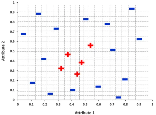
splitting the set of instances. In order to select the axis-parallel hyperplane, a greedy approach is used via im-purity measures of all axis-parallel hyperplanes (see Fig. 1). The hyperplane that provides the least impurity is chosen to be the splitting condition of the node. The algorithm stops when all instances are in the same class or user’s specified criteria are met.
Various impurity measures have been proposed for evaluating the performance of the hyperplane such as Gini [26] using in the well-known decision tree algo-rithm, CART [14]. Another decision tree algorithm like C4.5 [27] applies the Shannon’s entropy [28]. The Shan-non’s entropy used in OMCT algorithm is defined by (1). It equals to zero when all instances are in the same class and equals to one when the number of instances in all classes are identical.
Entropy(D) =−n + n log2 n+ n − n− n log2 n− n (1) 2.2.1. Decision Tree for Imbalanced Dataset
Traditional decision tree algorithms work well on the balanced datasets so they may not be appropriate for dealing with the imbalanced ones. Various impurity measures are proposed for improving the performance of the decision tree on the imbalanced datasets. In 2010, Chandra et al. presented the distinct class based splitting measure (DCSM) [29]. In 2006, the asymmetric entropy (AE) was proposed by Marcellin et al., [30]. The concept of the skew impurity measure is used instead of the sym-metric one such as Shannon’s entropy. The maximum value is shifted by the skewness parameterθbetween 0 and 1. Another skew impurity measure for the imbal-anced dataset is off-centered entropy (OCE) [31] that is suggested by Lenca et al., in 2008. In addition, the insen-sitive impurity measures are introduced for solving the class imbalanced problem such as DKM [32] and HDDT [33]. They are not affected by the ratio of the number of instances among all classes. Importantly, the technique that is an inspiration of this research is minority entropy (ME) [34]. It applies the concept of under-sampling in each node of the decision tree algorithm which is ex-plained below.
Minority Entropy
Minority entropy (ME) is proposed in 2016 by Boonchuay et al. [34]. For each attributej, the minor-ity rangeminrangej is defined as the interval between
the smallest and the largest values within attributejof minority instances. Then, the splitting step will only be examined within this rangeminrangej, i.e.
sprj(D) ={⃗x∈D|min⃗z∈D+projj(⃗z)
≤projj(⃗x)≤maxz⃗∈D+projj(⃗z)} (2)
Fig. 1. All axis-parallel hyperplanes (dash line) considering in a greedy approach.
Fig. 2. All axis-parallel hyperplanes (dash line) considering in ME. whereprojj(⃗a)is thejthelement of⃗a. It increases the
ratio of the minority instances for ensuring that the se-lected hyperplane from ME will separate the datasets in the region of the minority distribution, as shown in Fig. 2.
2.3. Oblique Decision Tree
For a small number of the distinct axis-parallel hy-perplanes, the greedy approach in a decision tree algo-rithm is practical. Nonetheless, the number of distinct oblique hyperplanes is up to2d·
(
n d
)
[13] having the ex-ponential number of hyperplanes to explore. Precisely,
this problem is proved to be NP-hard by Heath in 1993 [35]. Consequently, it is necessary to employ other tech-niques for finding the best oblique hyperplane. The lin-ear combination version of CART or CART-LC [14] uses a deterministic hill-climbing algorithm for finding the best oblique hyperplane. In 1993, Simulated An-nealing Decision Tree (SADT) is proposed by Heath et al. [11]. It applies the randomization of the simulated annealing algorithm to search for the best oblique hy-perplane. These two methodologies are combined to obtain the well-known oblique decision tree algorithm as Oblique Classifier 1 or OC1 [13] in 1994 which is the core algorithm of this research. There are some other effective techniques to solve this problem. The algo-rithms based on heuristic arguments such as OC1-GA and OC1-ES [19] use genetic algorithm and evolution-ary strategy to find the best oblique hyperplane, respec-tively. Using the feature extraction is another attractive concept. It transforms the original space before apply-ing the greedy approach to find the best axis-parallel hy-perplane such as the Fisher’s decision tree [17] and HH-CART [18].
Oblique Classifier 1
OC1 [13] is developed by Murthy et al. in 1994 for finding a multivariate split at each node of the decision tree algorithm. Two methodologies that are determinis-tic hill-climbing and randomization are used in selecting the split of the OC1 algorithm. It begins with the best axis-parallel hyperplane H : a0 +⃗a·⃗x = 0. Then,
this hyperplane is perturbed along each axis using deter-ministic hill-climbing. The greedy approach is applied on a set Uj, see (3), for finding the best new value of
coefficient aj. Geometrically, when replacingaj with
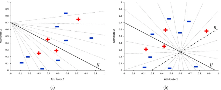
uij, thejth-intercept is shifted that will pass through the instance⃗xi. Fig. 3a shows all hyperplanes that are
con-sidered in deterministic hill-climbing with attribute 1.
Uj = { uij = −⃗a·⃗xi+aj ·x i j−a0 xi j |i= 1, ..., n } (3) However, the best hyperplane obtaining by this deter-ministic hill-climbing may get trap in the local solution. The randomization is offered to escape this local mini-mum. A random hyperplane R : r0 +⃗r ·⃗x = 0 is
generated by perturbingH withα, i.e. H+αR. The optimal value ofα is searched by the greedy approach on a setV defining by (4). Geometrically, eachvjgives a hyperplane that passes through instance⃗xiand the
inter-section ofHandR. All hyperplanes that are considered in randomization are shown in Fig. 3b.
V = { vi = −⃗a·⃗xi−a0 ⃗ r·⃗xi+r0 | i= 1, ..., n } (4)
3. Oblique Minority Condensed Decision Tree In this section, a novel oblique decision tree called minority condensed oblique decision tree or OMCT is proposed for handling the class imbalanced problem. It combines the oblique decision tree with the minority condensation.
3.1. Motivations
Although the axis-parallel decision tree algorithm based on minority entropy (ME) [34] shows the effec-tiveness of the decision tree algorithm for the class im-balanced problem. Nevertheless, class distribution of the real world datasets may not lie perfectly on any parallel axis so the best decision tree may not classify minority instances correctly. On the other hand, the oblique decision tree algorithm such as oblique classi-fier 1 (OC1) [13] uses a hyperplane that can deal with the oblique distribution. Oblique minority condensed decision tree (OMCT) integrates the advantages of ME and OC1 together. Furthermore, the disadvantage of each method is improved by the essence of one another. The minority condensation of minority instances is an essential ingredient of the OMCT algorithm. It is plied for condensing the minority instances before ap-plying the greedy approach in each step of OMCT: de-termining the best axis-parallel hyperplane, improving the minority entropy using deterministic hill-climbing on each axis, and improving the minority entropy by randomization. Moreover, extra caution to treat some minority instances that extremely deviate from the oth-ers, called outliers [36], is applied. The interquartile range rule [37] is deployed to discard the minority liers before applying the minority entropy. Values out-side the minority inner fence computed by[Q1−1.5∗
IQR, Q3+ 1.5∗IQR]of minority instances are treated
as the outliers and will be included after the partitioning step is done. The demonstration of the minority con-densation is shown by Fig. 4 with the Tukey boxplot of the minority instances in datasetX. It defines left mar-ginmland right marginmrby the largest and smallest
values of the minority instances within the minority in-ner fence of the current round. A set of instances within mlandmris denoted byM CX.
3.2. Minority Condensation
The formal definition of the minority condensation with some related formulae are defined in this section. Each instance both in minority and majority class is as-signed a score. The minority condensation keeps in-stances inside the inner fence of the Tukey boxplot ac-cording this score, see Definition 1.
(a) (b)
Fig. 3. Mechanism of perturbing the initial hyperplaneH(solid line) in each step of OC1 algorithm. (a) All hy-perplanes (dash line) considering in deterministic hill-climbing with attribute 1. (b) All hyhy-perplanes (dash line) considering in randomization with random hyperplaneR(solid-dash line).
Fig. 4. The overview of the minority condensation. Definition 1. Let X+ ⊂ R be a set of scores of the minority class. IQR is the interquartile range com-puted from the third quartileQ3 subtracting with the
first quartileQ1. DefineXwo+ ⊆X+without outliers as
follows:
Xwo+ ={x∈X+|Q1−1.5∗IQR≤x≤Q3+1.5∗IQR}
The core definition of this research, a set of scores with the minority condensation, is presented in
Defini-tion 2. It combines scores inXwo+ with the scores cor-responding to the majority instances where their values lie within the range ofXwo+.
Definition 2. LetX =X+∪X−be a set of scores of
all instances. A setX with the minority condensation is defined as follows:
M CX ={x∈X|ml ≤x≤mr}
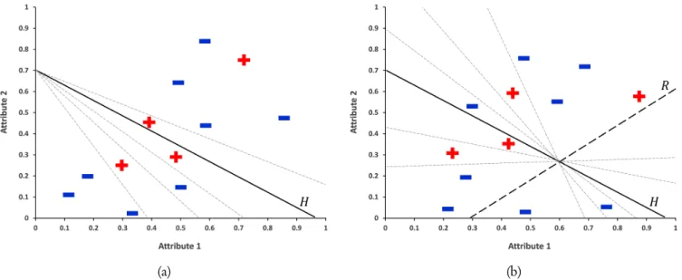
(a) (b)
Fig. 5. Applying the minority condensation to each step of the oblique decision tree algorithm, i.e. determinis-tic hill-climbing (a) and randomization (b).
the minimum and maximum values of Xwo+, respec-tively.
The set of scores from Definition 2 is constricted to intensify the importance of the instances in the mi-nority class. It is used in three steps of the OMCT al-gorithm. In the process of determining the best axis-parallel hyperplane, the minority condensation is ap-plied on each attribute of dataset D before the greedy approach. Minority instances that are discarded will be reconsidered in the next step. Due to the reduced range from the minority condensation, the number of discard majority instances is far more than ME. In the determin-istic hill-climbing, for eachjth the minority condensa-tion is applied on X where X is defined as Uj (3). It
reduces the number of considered hyperplanes by a⃗a withoutjthcomponent, see Fig. 5a. For improving the minority entropy by randomization, the minority con-densation is applied onX whereX is defined asV (4). It also reduces the number of considered hyperplanes at the intersection of given hyperplaneHand the random hyperplane, see Fig. 5b.
3.3. OMCT Algorithm
The OMCT algorithm is constructed in a top-down fashion [38]. It separates the instances into two parti-tions using the oblique hyperplane as a criterion. Then, it recursively repeats on each partition until only one class instances are left in the partition or other specified stopping criteria are met.
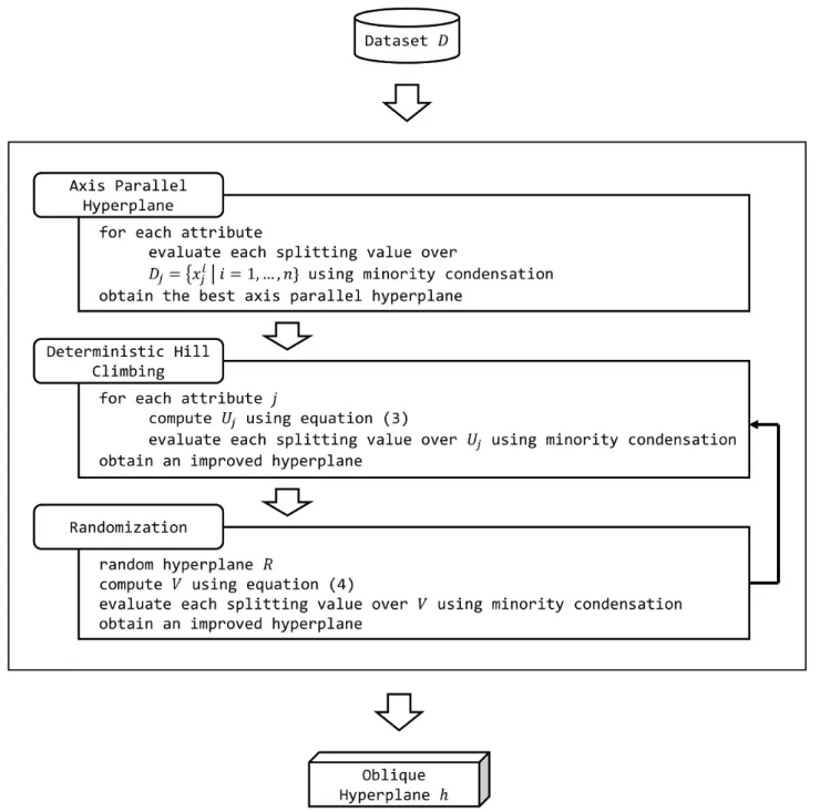
The steps of the OMCT algorithm, which employs to search for an optimal oblique hyperplane, is illus-trated by Fig. 6. It starts with calling the Axis Parallel Hyperplane step to generate the initial axis parallel hy-perplane. The deterministic hill climbing step is applied
to each attribute, which is restricted to the region of mi-nority class by using the mimi-nority condensation. Then, it perturbs the hyperplane using the deterministic hill climbing step and the randomization step respectively. The use of the minority condensation is embedded in all steps to reduce the set of considered instances. They are repeated in a loop until the obtained oblique hyperplane cannot be improved.
Time Complexity of the Minority Condensation The time complexity analysis of the minority con-densation is shown in this section. There are three parts for applying the minority condensation to the set of scoresXof sizen. First, separating the class of instances inXto the minority or majority classes usesO(n)time complexity. Second, determining the setXwo+ by Defi-nition 1 takesO(n log n)running time using the merge sort for calculating the minority inner fence. Third, defining the setM CX by Definition 2 spendsO(n)for
considering that each instance is either inside or outside the interval betweenmlandmr. In summary, the
over-all time complexity is O(n) +O(n log n) +O(n) =
O(n log n)running time.
4. Experiments
This section purposes performance comparisons in classifying the imbalance datasets of OMCT with other effective decision tree algorithms in two aspects, the per-formance of classification and the size of a decision tree.
Fig. 6. Brief pseudo codes and basic iterations of the OMCT algorithm.
4.1. Datasets
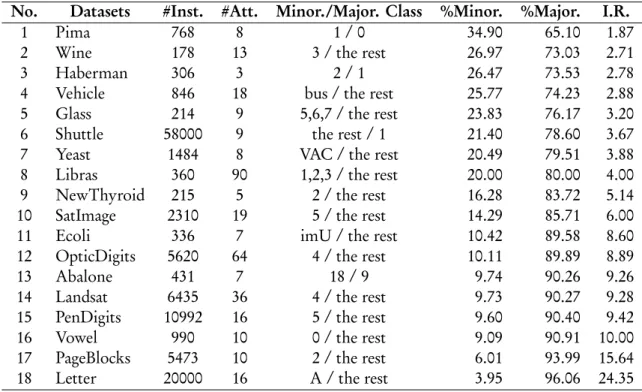
In order to evaluate the performance of OMCT comparing with other decision tree algorithms, the real-world datasets from UCI repository [39] are used as ex-perimental benchmark. Table 1 shows the summary of each dataset using in the experiments. The number and the name of each dataset appear in the first and the sec-ond columns, while the third and the fourth columns show the number of instances and the number of at-tributes. The fifth column presents the selected class for labeling as the minority class and the majority class. For the last three columns, they contain the percentage of the minority class, the majority class and the ratio of them called the imbalanced ratio, respectively. Each
dataset applies the five-fold cross-validation and repeats it 20 times. Hence, one hundred experiments are per-formed on each dataset.
4.2. Comparative Methods and Evaluation
The performance of OMCT is evaluated compar-ing with six decision tree algorithms. Two out of six are well-known axis-parallel decision tree algorithms, CART [14] and C4.5 [27]. Others are the most famous oblique decision tree algorithm as OC1 [13], and three state-of-art decision tree algorithms for an imbalanced dataset, i.e. AE [30], DCSM [29] and ME [34].
There are two aspects to report in this paper which are (1) classification performances and (2) tree sizes. Due
Table 1. Summary of experimental datasets.
No. Datasets #Inst. #Att. Minor./Major. Class %Minor. %Major. I.R.
1 Pima 768 8 1 / 0 34.90 65.10 1.87
2 Wine 178 13 3 / the rest 26.97 73.03 2.71
3 Haberman 306 3 2 / 1 26.47 73.53 2.78
4 Vehicle 846 18 bus / the rest 25.77 74.23 2.88
5 Glass 214 9 5,6,7 / the rest 23.83 76.17 3.20
6 Shuttle 58000 9 the rest / 1 21.40 78.60 3.67
7 Yeast 1484 8 VAC / the rest 20.49 79.51 3.88
8 Libras 360 90 1,2,3 / the rest 20.00 80.00 4.00 9 NewThyroid 215 5 2 / the rest 16.28 83.72 5.14 10 SatImage 2310 19 5 / the rest 14.29 85.71 6.00
11 Ecoli 336 7 imU / the rest 10.42 89.58 8.60
12 OpticDigits 5620 64 4 / the rest 10.11 89.89 8.89
13 Abalone 431 7 18 / 9 9.74 90.26 9.26
14 Landsat 6435 36 4 / the rest 9.73 90.27 9.28
15 PenDigits 10992 16 5 / the rest 9.60 90.40 9.42
16 Vowel 990 10 0 / the rest 9.09 90.91 10.00
17 PageBlocks 5473 10 2 / the rest 6.01 93.99 15.64 18 Letter 20000 16 A / the rest 3.95 96.06 24.35
to the extreme difference number of instances in each class, the traditional measure like accuracy is not suit-able to evaluate the performance of classifying imbal-anced datasets. It shows the detection rate of a whole dataset that has the minimum affect when the instances in the minority class are misclassified. In considering the binary class imbalanced problem, two performance aspects need to be evaluated, i.e., the percentage of in-stances correctly predicted to be the minority class and the percentage of the minority instances that are cor-rectly classified. They are represented by two widely used measures which are precision and recall defined by equations (5) and (6), respectively [40]. Moreover, their harmonic mean, represented by F1 score in equation (7), summarizes the overall performance of each classifier. For the size of each decision tree, it is measured by the number of leaf nodes referring to the number of parti-tions. The smaller the number of nodes in a decision tree, the smaller the number of partitions.
P recision= T P T P +F P (5) Recall= T P T P +F N (6) F1 = 2· P recision·Recall P recision+Recall (7) where
• T P is the number of true predicted of minority instances.
• F P is the number of false predicted of minority instances.
• T N is the number of true predicted of majority instances.
• F N is the number of false predicted of majority instances.
In addition, the non-parametric statistical hypothe-sis test as Wilcoxon signed-rank test with 0.01 and 0.05 significance level (α) is applied for testing the perfor-mance difference of OMCT comparing with other al-gorithms. The null hypothesis (H0) and the alternative
hypothesis (H1) of Wilcoxon signed-rank test are indi-cated as follows.
H0:The performance of OMCT and the comparative
method are not different.
H1:The performance of OMCT and the comparative
method are different. 4.3. Results and Discussions
The experimental results are demonstrated in this section. Each table shows the experimental results with different measurements. Each row of the table reports the performance of each decision tree algorithm work-ing on the specific dataset.
4.3.1. Classification Performances
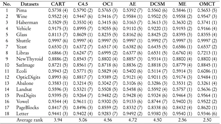
In the first experimental result, the precision of each decision tree algorithm is shown in Table 2. OMCT yields the least average ranking over other methods that
stances by other algorithms. Especially, the decision tree algorithms designing for the imbalanced datasets such as AE and DCSM show the poor recall. This happens because that they focus on the minority in-stances excessively causing the boundary of partitioning to overfit the minority class.
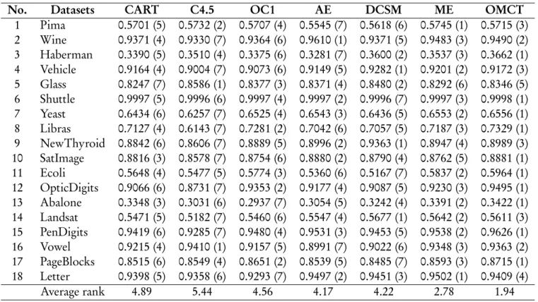
The performance of each decision tree algorithm for handling the class imbalanced problem is represented by F1 score as in Table 4. Since OMCT has the low-est ranking in both precision and recall, it provides the best ranking in F1 score also. Statistically, the F1 score of OMCT is significantly better than CART, C4.5 and OC1 with a 99% confidence level. Note that those decision tree algorithms show poor performance since they are not designed for imbalanced datasets. For the decision tree algorithms inventing for the imbalanced dataset specifically such as AE, DCSM and ME, they have the lower performances than OMCT significantly as well at a 95% confidence level.
All experiments in this paper confirm that the pro-posed decision tree algorithm, OMCT, offers the im-provement over other decision tree algorithms. Espe-cially, it outperforms OC1 and ME which originate the concept of OMCT. Although OC1 shows the improve-ment over the traditional decision tree in both preci-sion and recall, neglecting the importance of the mi-nority class causes OC1 to misclassify a lot of mimi-nority instances, resulting in a low precision. ME shows the outstanding ability to discover the minority instances which is observed by the recall. Nevertheless, it gives low precision due to the unnecessarily broad range of minority instances. It results in the partitioning bound-ary of minority instances locates within the region of the majority class. OMCT integrates the advantages of both concepts, which consists of applying the oblique hyperplane to capture the distribution of the dataset, concentrating on the minority instances like ME to in-crease the chance of classifying minority instances, and avoiding outliers to reduce the affect of the broader range.
partitions of OMCT than other methods. The reason is due to the ability in capturing the distribution of the minority class via the minority condensation and the flexibility of the oblique hyperplane. For the same rea-sons, applying the minority range of ME and using the oblique hyperplane of OC1 make tree size comparison to be within the second or the third ranks in this ex-periment. They have the similar number of leaf nodes, which are less than other methods, but they are still larger than OMCT significantly.
5. Conclusions
A novel oblique decision tree for handling the class imbalanced problem called oblique minority condensed decision tree or OMCT is introduced in this paper, which is an enhancement of the well-known oblique decision tree like OC1. The proposed minority con-densation is embedded in the greedy approach for defin-ing the boundary of minority instances within their cluster using the inner fence selection. OMCT is able to handle the class imbalanced problem by recursive partitioning the dataset using the combination of at-tributes, which concentrates on the region of the mi-nority class. Although it requires additional process for determining the minority condensation. However, it takesO(nlog(n))time complexity indistinguishable with the greedy approach without the minority conden-sation. Moreover, the number of splitting values that need to be considered is decreased when applying the minority condensation. At each node of the oblique de-cision tree algorithm, the greedy approach with the mi-nority condensation is applied in three steps of building decision tree, i.e. to find the best axis-parallel hyper-plane, to perturb the hyperplane along each axis with deterministic hill-climbing and to avoid the local solu-tion with randomizasolu-tion.
The experimental results show that OMCT signif-icantly outperforms CART, C4.5, OC1, AE, DCSM and ME in term of F1 score on eighteen real-world
im-Table 2. The performance comparison of precision on imbalanced datasets including with the rank which is shown in the parentheses.
No. Datasets CART C4.5 OC1 AE DCSM ME OMCT
1 Pima 0.5712 (3) 0.5708 (4) 0.5683 (6) 0.5739 (2) 0.5707 (5) 0.5681 (7) 0.5808 (1) 2 Wine 0.9293 (6) 0.9302 (5) 0.9387 (4) 0.9673 (1) 0.9291 (7) 0.9460 (3) 0.9485 (2) 3 Haberman 0.3343 (7) 0.3569 (3) 0.3446 (6) 0.3504 (5) 0.3678 (1) 0.3543 (4) 0.3666 (2) 4 Vehicle 0.9179 (5) 0.9041 (7) 0.9116 (6) 0.9211 (3) 0.9360 (1) 0.9232 (2) 0.9195 (4) 5 Glass 0.8556 (5) 0.8705 (2) 0.8662 (3) 0.8747 (1) 0.8652 (4) 0.8381 (7) 0.8493 (6) 6 Shuttle 0.9997 (6) 0.9996 (7) 0.9997 (5) 0.9998 (3) 0.9999 (1) 0.9998 (4) 0.9998 (2) 7 Yeast 0.6391 (6) 0.6182 (7) 0.6567 (3) 0.6756 (1) 0.6486 (5) 0.6553 (4) 0.6595 (2) 8 Libras 0.7553 (6) 0.6205 (7) 0.7765 (4) 0.8067 (1) 0.7892 (2) 0.7841 (3) 0.7554 (5) 9 NewThyroid 0.8948 (6) 0.8819 (7) 0.9107 (5) 0.9288 (2) 0.9500 (1) 0.9215 (4) 0.9275 (3) 10 SatImage 0.8929 (3) 0.8611 (7) 0.8805 (4) 0.8939 (1) 0.8780 (5) 0.8765 (6) 0.8930 (2) 11 Ecoli 0.5893 (4) 0.5570 (7) 0.6065 (3) 0.5666 (5) 0.5641 (6) 0.6164 (1) 0.6079 (2) 12 OpticDigits 0.9148 (6) 0.8655 (7) 0.9321 (2) 0.9240 (4) 0.9173 (5) 0.9293 (3) 0.9512 (1) 13 Abalone 0.3277 (4) 0.3064 (6) 0.3031 (7) 0.3169 (5) 0.3417 (3) 0.3434 (2) 0.3820 (1) 14 Landsat 0.5374 (6) 0.5073 (7) 0.5428 (5) 0.5661 (2) 0.5792 (1) 0.5556 (4) 0.5608 (3) 15 PenDigits 0.9446 (6) 0.9310 (7) 0.9480 (5) 0.9639 (2) 0.9587 (4) 0.9616 (3) 0.9691 (1) 16 Vowel 0.9135 (5) 0.9260 (3) 0.9063 (6) 0.8918 (7) 0.9400 (1) 0.9344 (2) 0.9247 (4) 17 PageBlocks 0.8634 (6) 0.8622 (7) 0.8758 (4) 0.8785 (2) 0.8654 (5) 0.8781 (3) 0.8830 (1) 18 Letter 0.9362 (5) 0.9320 (6) 0.9307 (7) 0.9508 (2) 0.9528 (1) 0.9467 (4) 0.9477 (3) Average rank 5.28 5.89 4.72 2.72 3.22 3.67 2.50
Table 3. The performance comparison of recall on imbalanced datasets including with the rank which is shown in the parentheses.
No. Datasets CART C4.5 OC1 AE DCSM ME OMCT
1 Pima 0.5738 (4) 0.5790 (2) 0.5765 (3) 0.5392 (7) 0.5560 (6) 0.5846 (1) 0.5653 (5) 2 Wine 0.9522 (4) 0.9447 (6) 0.9416 (7) 0.9584 (1) 0.9502 (5) 0.9558 (2) 0.9547 (3) 3 Haberman 0.3509 (5) 0.3530 (4) 0.3415 (6) 0.3163 (7) 0.3613 (3) 0.3630 (2) 0.3741 (1) 4 Vehicle 0.9175 (3) 0.8995 (7) 0.9055 (6) 0.9110 (5) 0.9220 (1) 0.9193 (2) 0.9166 (4) 5 Glass 0.8113 (7) 0.8609 (1) 0.8235 (5) 0.8162 (6) 0.8425 (2) 0.8395 (3) 0.8355 (4) 6 Shuttle 0.9997 (6) 0.9997 (4) 0.9997 (5) 0.9997 (1) 0.9992 (7) 0.9997 (3) 0.9997 (2) 7 Yeast 0.6530 (3) 0.6372 (7) 0.6517 (4) 0.6382 (6) 0.6435 (5) 0.6586 (1) 0.6537 (2) 8 Libras 0.6866 (3) 0.6247 (7) 0.6995 (2) 0.6377 (6) 0.6531 (5) 0.6760 (4) 0.7213 (1) 9 NewThyroid 0.8886 (2) 0.8543 (7) 0.8800 (4) 0.8857 (3) 0.9314 (1) 0.8800 (4) 0.8800 (4) 10 SatImage 0.8721 (5) 0.8561 (7) 0.8718 (6) 0.8836 (2) 0.8818 (3) 0.8779 (4) 0.8845 (1) 11 Ecoli 0.5943 (2) 0.5771 (5) 0.5829 (4) 0.5400 (6) 0.5114 (7) 0.5914 (3) 0.6086 (1) 12 OpticDigits 0.8993 (6) 0.8817 (7) 0.9389 (2) 0.9121 (4) 0.9011 (5) 0.9174 (3) 0.9484 (1) 13 Abalone 0.3583 (1) 0.3214 (5) 0.3042 (7) 0.3106 (6) 0.3286 (3) 0.3531 (2) 0.3261 (4) 14 Landsat 0.5596 (3) 0.5321 (7) 0.5508 (5) 0.5458 (6) 0.5592 (4) 0.5757 (1) 0.5636 (2) 15 PenDigits 0.9395 (5) 0.9264 (7) 0.9482 (2) 0.9428 (4) 0.9324 (6) 0.9464 (3) 0.9564 (1) 16 Vowel 0.9344 (4) 0.9611 (1) 0.9300 (5) 0.9133 (6) 0.8744 (7) 0.9400 (3) 0.9522 (2) 17 PageBlocks 0.8417 (5) 0.8496 (3) 0.8559 (2) 0.8332 (7) 0.8338 (6) 0.8432 (4) 0.8620 (1) 18 Letter 0.9441 (3) 0.9402 (4) 0.9283 (7) 0.9492 (2) 0.9380 (5) 0.9540 (1) 0.9346 (6) Average rank 3.94 5.06 4.56 4.72 4.50 2.56 2.50
balanced datasets from UCI. It shows the precision im-provement in classifying the minority instances over the traditional decision tree algorithms. For the recall, it fixes the overfitting problem found in the decision tree
algorithms for class imbalanced datasets. In addition, OMCT offers the smallest size of the decision tree in term of the number of leaf nodes which implies that the decision tree from OMCT is more general than other
10 SatImage 0.8816 (3) 0.8578 (7) 0.8754 (6) 0.8880 (2) 0.8790 (4) 0.8762 (5) 0.8881 (1) 11 Ecoli 0.5648 (4) 0.5477 (5) 0.5774 (3) 0.5360 (6) 0.5167 (7) 0.5837 (2) 0.5964 (1) 12 OpticDigits 0.9066 (6) 0.8731 (7) 0.9353 (2) 0.9177 (4) 0.9087 (5) 0.9230 (3) 0.9495 (1) 13 Abalone 0.3348 (3) 0.3031 (6) 0.2937 (7) 0.3054 (5) 0.3242 (4) 0.3391 (2) 0.3422 (1) 14 Landsat 0.5471 (5) 0.5182 (7) 0.5460 (6) 0.5547 (4) 0.5677 (1) 0.5642 (2) 0.5611 (3) 15 PenDigits 0.9419 (6) 0.9285 (7) 0.9480 (4) 0.9531 (3) 0.9453 (5) 0.9538 (2) 0.9626 (1) 16 Vowel 0.9215 (4) 0.9410 (1) 0.9157 (5) 0.8991 (7) 0.9022 (6) 0.9348 (3) 0.9363 (2) 17 PageBlocks 0.8515 (6) 0.8549 (4) 0.8651 (2) 0.8539 (5) 0.8485 (7) 0.8593 (3) 0.8715 (1) 18 Letter 0.9398 (5) 0.9358 (6) 0.9293 (7) 0.9497 (2) 0.9451 (3) 0.9502 (1) 0.9409 (4) Average rank 4.89 5.44 4.56 4.17 4.22 2.78 1.94
Table 5. The comparison of tree size on imbalanced datasets including with the rank which is shown in the parentheses.
No. Datasets CART C4.5 OC1 AE DCSM ME OMCT
1 Pima 110.64 (4) 146.62 (7) 83.98 (2) 125.12 (5) 145.10 (6) 104.48 (3) 75.02 (1) 2 Wine 4.56 (6) 4.56 (6) 4.32 (5) 3.70 (1) 4.10 (4) 3.96 (3) 3.78 (2) 3 Haberman 79.68 (3) 87.22 (7) 58.14 (2) 81.78 (5) 86.52 (6) 79.74 (4) 54.22 (1) 4 Vehicle 25.62 (5) 34.34 (7) 25.26 (4) 27.08 (6) 23.68 (3) 22.10 (2) 18.62 (1) 5 Glass 10.10 (5) 10.48 (6) 9.74 (3) 10.84 (7) 9.86 (4) 9.60 (2) 9.28 (1) 6 Shuttle 22.14 (5) 29.02 (7) 22.24 (6) 19.34 (4) 16.20 (2) 16.60 (3) 16.10 (1) 7 Yeast 132.56 (4) 155.34 (6) 109.02 (2) 142.96 (5) 167.24 (7) 124.44 (3) 99.94 (1) 8 Libras 21.48 (5) 38.44 (7) 20.90 (4) 21.70 (6) 18.84 (3) 17.58 (2) 16.14 (1) 9 NewThyroid 6.52 (5) 8.30 (7) 6.36 (4) 7.14 (6) 5.20 (1) 5.96 (3) 5.62 (2) 10 SatImage 54.46 (5) 70.26 (7) 51.26 (3) 55.82 (6) 53.18 (4) 48.54 (2) 40.82 (1) 11 Ecoli 20.12 (4) 22.42 (6) 17.36 (2) 21.12 (5) 23.42 (7) 18.18 (3) 16.02 (1) 12 OpticDigits 65.58 (5) 101.86 (7) 19.74 (2) 55.24 (4) 73.58 (6) 48.34 (3) 13.76 (1) 13 Abalone 36.14 (4) 43.16 (6) 33.48 (3) 36.76 (5) 44.90 (7) 33.08 (2) 29.86 (1) 14 Landsat 252.50 (4) 368.84 (7) 204.74 (2) 267.54 (5) 322.00 (6) 218.50 (3) 171.32 (1) 15 PenDigits 95.26 (6) 123.46 (7) 51.76 (2) 73.12 (4) 92.22 (5) 66.62 (3) 31.48 (1) 16 Vowel 13.40 (6) 13.26 (5) 12.02 (3) 16.18 (7) 13.16 (4) 9.58 (2) 9.32 (1) 17 PageBlocks 67.56 (4) 77.54 (6) 48.80 (2) 69.56 (5) 86.34 (7) 61.72 (3) 44.16 (1) 18 Letter 87.30 (5) 106.30 (6) 68.96 (2) 80.84 (4) 117.76 (7) 71.26 (3) 48.88 (1) Average rank 4.72 6.50 2.94 5.00 4.94 2.72 1.11 methods.
For some imbalance datasets such as Glass and Let-ter, OMCT has lower rank than other decision tree al-gorithms. It is conceivable that the local best split at the
current step may not lead to the optimal decision tree [41]. Inducing the tree with an imperfect split at the be-ginning may result in the lower misclassified tree at the end. Furthermore, the use of oblique hyperplane may
not handle the minority instances having spherical dis-tribution perfectly since any oblique hyperplanes can be used to split this dataset.
Due to the complexity of finding the best oblique hyperplane, the algorithms for constructing OMCT takes long time to converge. Some improvements are needed for handling this situation. Moreover, the mul-ticlass imbalanced problem with the nominal attributes should be investigated using OMCT technique.
Acknowledgments
The authors would like to thank for a support in part from the Science Achievement Scholarship of Thai-land (SAST) and the Applied Mathematics and Compu-tational Science Program in the Department of Mathe-matics and Computer Science, Faculty of Science, Chu-lalongkorn University, Thailand.
References
[1] V. López, A. Fernández, S. García, V. Palade, and F. Herrera, “An insight into classification with im-balanced data: Empirical results and current trends on using data intrinsic characteristics,”Information Sciences, vol. 250, pp. 113–141, 2013.
[2] S. Panigrahi, A. Kundu, S. Sural, and A. K. Ma-jumdar, “Credit card fraud detection: A fusion ap-proach using dempster–shafer theory and bayesian learning,” Information Fusion, vol. 10, no. 4, pp. 354–363, 2009.
[3] W. Wei, J. Li, L. Cao, Y. Ou, and J. Chen, “Ef-fective detection of sophisticated online banking fraud on extremely imbalanced data,”World Wide Web, vol. 16, no. 4, pp. 449–475, 2013.
[4] B. Krawczyk, M. Galar, Ł. Jeleń, and F. Herrera, “Evolutionary undersampling boosting for imbal-anced classification of breast cancer malignancy,”
Applied Soft Computing, vol. 38, pp. 714–726, 2016. [5] S.-H. Bae and K.-J. Yoon, “Polyp detection via im-balanced learning and discriminative feature learn-ing,”IEEE transactions on medical imaging, vol. 34, no. 11, pp. 2379–2393, 2015.
[6] S. Jaiyen and P. Sornsuwit, “A new incremental decision tree learning for cyber security based on ilda and mahalanobis distance,” Engineering Jour-nal, vol. 23, no. 5, pp. 71–88, 2019.
[7] P. C. Lane, D. Clarke, and P. Hender, “On de-veloping robust models for favourability analysis: Model choice, feature sets and imbalanced data,”
Decision Support Systems, vol. 53, no. 4, pp. 712– 718, 2012.
[8] L. Song, D. Li, X. Zeng, Y. Wu, L. Guo, and Q. Zou, “ndna-prot: identification of dna-binding proteins based on unbalanced classification,”BMC bioinformatics, vol. 15, no. 1, p. 298, 2014.
[9] S. M. Pourhashemi, “E-mail spam filtering by a new hybrid feature selection method using chi2 as filter and random tree as wrapper,”Engineering Journal, vol. 18, no. 3, pp. 123–134, 2014.
[10] A. Fernández, S. García, M. Galar, R. C. Prati, B. Krawczyk, and F. Herrera, Learning from im-balanced data sets. Springer, 2018.
[11] D. Heath, S. Kasif, and S. Salzberg, “Induction of oblique decision trees,” in IJCAI, vol. 1993, 1993, pp. 1002–1007.
[12] K. J. Cios, W. Pedrycz, R. W. Swiniarski, and L. A. Kurgan, Data mining: a knowledge discovery ap-proach. Springer Science & Business Media, 2007. [13] S. K. Murthy, S. Kasif, and S. Salzberg, “A system for induction of oblique decision trees,”Journal of artificial intelligence research, vol. 2, pp. 1–32, 1994. [14] L. Breiman, Classification and regression trees.
Routledge, 2017.
[15] M. F. Amasyali and O. Ersoy, “Cline: A new decision-tree family,” IEEE Transactions on Neural Networks, vol. 19, no. 2, pp. 356–363, 2008. [16] B. Robertson, C. Price, and M. Reale, “Cartopt:
a random search method for nonsmooth uncon-strained optimization,” Computational Optimiza-tion and ApplicaOptimiza-tions, vol. 56, no. 2, pp. 291–315, 2013.
[17] A. LóPez-Chau, J. Cervantes, L. LóPez-GarcíA, and F. G. Lamont, “Fisher’s decision tree,”Expert Systems with Applications, vol. 40, no. 16, pp. 6283– 6291, 2013.
[18] D. Wickramarachchi, B. Robertson, M. Reale, C. Price, and J. Brown, “Hhcart: An oblique de-cision tree,”Computational Statistics & Data Anal-ysis, vol. 96, pp. 12–23, 2016.
[19] E. Cantu-Paz and C. Kamath, “Inducing oblique decision trees with evolutionary algorithms,”IEEE Transactions on Evolutionary Computation, vol. 7, no. 1, pp. 54–68, 2003.
[20] M. Chabbouh, S. Bechikh, C.-C. Hung, and L. B. Said, “Multi-objective evolution of oblique de-cision trees for imbalanced data binary classifi-cation,” Swarm and Evolutionary Computation, 2019.
[21] C. Bunkhumpornpat and K. Sinapiromsaran, “Dbmute: density-based majority under-sampling technique,” Knowledge and Information Systems, vol. 50, no. 3, pp. 827–850, 2017.
[22] N. V. Chawla, K. W. Bowyer, L. O. Hall, and W. P. Kegelmeyer, “Smote: synthetic minority
bles for the class imbalance problem: bagging-, boosting-, and hybrid-based approaches,” IEEE Transactions on Systems, Man, and Cybernetics, Part C (Applications and Reviews), vol. 42, no. 4, pp. 463–484, 2011.
[26] C. Gini, “Variability and mutability, contribution to the study of statistical distributions and rela-tions. studi cconomico-giuridici della r. universita de cagliari (1912). reviewed in: Light, rj, margolin, bh: An analysis of variance for categorical data,”J. American Statistical Association, vol. 66, pp. 534– 544, 1971.
[27] J. R. Quinlan,C4. 5: programs for machine learning. Elsevier, 2014.
[28] C. E. Shannon, “A mathematical theory of com-munication,”Bell system technical journal, vol. 27, no. 3, pp. 379–423, 1948.
[29] B. Chandra, R. Kothari, and P. Paul, “A new node splitting measure for decision tree construction,”
Pattern Recognition, vol. 43, no. 8, pp. 2725–2731, 2010.
[30] S. Marcellin, D. A. Zighed, and G. Ritschard, “An asymmetric entropy measure for decision trees,” 2006.
[31] P. Lenca, S. Lallich, T.-N. Do, and N.-K. Pham, “A comparison of different off-centered entropies
entropy for the class imbalance problem,”Pattern Analysis and Applications, vol. 20, no. 3, pp. 769– 782, 2017.
[35] D. G. Heath, “A geometric framework for ma-chine learning,” 1993.
[36] D. M. Hawkins, Identification of outliers. Springer, 1980, vol. 11.
[37] J. W. Tukey, Exploratory data analysis. Reading, Mass., 1977, vol. 2.
[38] L. Rokach and O. Maimon, “Top-down induction of decision trees classifiers-a survey,”IEEE Transac-tions on Systems, Man, and Cybernetics, Part C (Ap-plications and Reviews), vol. 35, no. 4, pp. 476–487, 2005.
[39] C. L. Blake, “Uci repository of machine learn-ing databases, irvine, university of california,”
http://www. ics. uci. edu/~ mlearn/MLRepository. html, 1998.
[40] M. Buckland and F. Gey, “The relationship be-tween recall and precision,” Journal of the Ameri-can society for information science, vol. 45, no. 1, pp. 12–19, 1994.
[41] V. S. Iyengar, “Hot: Heuristics for oblique trees,” in Proceedings 11th International Conference on Tools with Artificial Intelligence. IEEE, 1999, pp. 91–98.
Appendix
Algorithm 1OMCT (D,C,J)
Require: Dataset D= {⃗x1, ⃗x2, ..., ⃗xn}with respect to the set of classesC = {c1, c2, ..., cn}and the number of
using randomizationJ.
1: Creating a node of the tree.
ifAll instances are in the same class.then return The node labeled as that class. end if 2: H:a0+⃗a·⃗x= 0 =ObliqueHyperplane (D,C,J) 3: Dl=∅ 4: Cl =∅ 5: Dr =∅ 6: Cr =∅ fori= 1, ..., ndo ifa0+⃗a·⃗xi≤0then 7: Dl=Dl∪ {⃗xi} 8: Cl=Cl∪ {ci} else 9: Dr=Dr∪ {⃗xi} 10: Cr =Cr∪ {ci} end if end for 11: OMCT (Dl,Cl,J) 12: OMCT (Dr,Cr,J) Algorithm 2ObliqueHyperplane (D,C,J)
Require: The set of instancesDwith respect to the set of classesCand the number of using randomizationJ. 1: H, I =AxisParallelHyperplane (D,C) 2: H, I =DeterministicHillClimbing (D,C,H,I) 3: count= 1 whilecount≤5do 4: H′, I′ =Randomization (D,C,H,I) ifI′< I then 5: I =I′ 6: H =H′ 7: H, I =DeterministicHillClimbing (D,C,H,I) 8: count= 0 end if 9: count+ = 1 end while return H
ifI′< I then 8: I =I′
9: SelectedAttr=j
10: SelectedV alue=BestSplit end if
end for
11: Defining hyperplaneH:a0+⃗a·⃗x= 0, where all coefficients of⃗aare 0, except forSelectedAttrth element
is 1, anda0 =−SelectedV alue.
return H,I
Algorithm 4DeterministicHillClimbing (D,C,H,I)
Require: The set of instancesDwith respect to the set of classesC, the hyperplaneHand the impurityI. forj= 1, ..., ddo
1: ComputingUj using (3)
2: M CU =MinorityCondensation(Uj,C)
3: LetBestSplit∈M CUbe the best splitting value ofM CUobtaining from the greedy approach onM CU.
4: LetI′ be the Shannon’s entropy of partitioningM CU withBestSplit.
ifI′< I then 5: I =I′ 6: aj =BestSplit end if end for return H,I Algorithm 5Randomization (D,C,H)
Require: The set of instancesDwith respect to the set of classesCand the hyperplaneH. 1: Randomly hyperplaneR :r0+⃗a·⃗r= 0
2: ComputingV using (4)
3: M CV =MinorityCondensation(V,C)
4: Letα∈M CV be the best splitting value ofM CV obtaining from the greedy approach onM CV.
5: LetI′be the Shannon’s entropy of partitioningM CV withα.
6: Defining hyperplaneH′ :H+αR return H′,I′
Algorithm 6MinorityCondensation (X,C)
Require: The set of score X = {x1, x2, ..., xk} with respect to the set of classes C = {c1, c2, ..., ck} where
ci ∈ {+1,−1}.
1: X+={xi∈D|ci= +1}
2: LetM inP osbe the minimum value ofX+. 3: LetQ1P osbe the first quartile ofX+.
4: LetQ3P osbe the third quartile ofX+.
5: LetM axP osbe the maximum value ofX+. 6: IQR=Q3P os−Q1P os
7: Xwo+ ={xi ∈X+|Q1P os−1.5∗IQR≤xi ≤Q3P os+ 1.5∗IQR}(Definition 1)
8: Letmlbe the minimum value ofXwo+.
9: Letmrbe the maximum value ofXwo+.
11: M CX ={xi∈X|ml≤xi≤mr}(Definition 2)
return M CX
Artit Sagoolmuang received the B.Sc. degrees (first-class honours) in Mathematics from Kasetsart University, Bangkok, Thailand, in 2014 and the M.S. degree in Applied Mathe-matics and Computational Science from Chulalongkorn University, Bangkok, Thailand, in 2016. Since 2017, he has been a Ph.D. candidate in Applied Mathematics and Computational Science program at Chulalongkorn University. His research interests include data mining and machine Learning algorithm especially in handling the class imbalanced problem.
Krung Sinapiromsaranreceived his B.S. in Mathematics from Chulalongkorn University, his M.S. and Ph.D. in Computer Science from the University of Wisconsin-Madison. He is currently an Assistant Professor in the Department of Mathematics, Chulalongkorn Uni-versity. His ongoing research works are related to deep learning, machine learning, artificial intelligence, data mining, knowledge discovery, and optimization.