IEO Background Paper
INDEPENDENT EVALUATION OFFICE
INTERNATIONAL MONETARY FUND
Social Spending in IMF-Supported
Programs
Ricardo Martin and Alex Segura-Ubiergo
The views expressed in this Background Paper are those of the author(s) and do not necessarily represent those of the IMF, IMF policy or the IEO. Background Papers report analyses related to the work of the IEO and are published to elicit comments and to further debate.
© 2004 International Monetary Fund BP/04/1
IEO Background Paper
Independent Evaluation Office
Social Spending in IMF-Supported Programs
Prepared by Ricardo Martin and Alex Segura-Ubiergo April 2004
Abstract
The views expressed in this Background Paper are those of the author(s) and do not necessarily represent those of the IMF, IMF policy or the IEO. Background Papers report analyses related to the work of the IEO and are published to elicit comments and to further debate.
This paper analyzes social spending in IMF-supported programs using a data base on public health and education spending for 146 countries over the 1985–2000 period. It uses
Autoregressive Integrated Moving Average (ARIMA) model techniques as well as a two-stage estimation method to obtain parameter estimates and correct for the endogeneity of Fund programs. Contrary to common perception, our findings show that social spending does not decline under IMF-supported programs. However, this does not necessarily mean that the most vulnerable groups are protected from the effects of economic adjustment.
JEL Classification Numbers: C33, E62, H51, H52 Keywords: IMF, social spending, fiscal policy
Contents Page
I. Introduction...3
II. Determinants of Social Expenditures and the Impact of IMF-Supported Programs ...4
III. The Impact of IMF-Supported Programs on Social Spending: A Time-Series Cross-Section Analysis...10
IV. Results...14
V. Robustness of the Results ...15
VI. Conclusions...18
I. INTRODUCTION
Critics of the Fund have argued that IMF policy recommendations with their emphasis on fiscal adjustment—through a combination of tax increases and seemingly drastic reductions in public expenditures—have had a devastating effect on the poor. For example, Naiman and Watkins (1999) of the Center for Economic and Policy Research have argued that “there is an urgent need for increased attention to the provision of basic social services. However, IMF adjustment programs restrict access to health services and public education in two key ways: by reducing household incomes, and by reducing public (government) spending”. Similarly, the Bretton Woods Project (2004), a well-known critic of Washington-based international financial institutions notes that “in the face of public exhortations to greater spending on social services, low income country governments however find themselves trapped by Fund diktat on budget balances, inflation and interest rates.” Other NGO’s such as Global
Exchange (2001) have pointed out that “the subordination of social needs to the concerns of financial markets has made it more difficult for national governments to ensure that their people receive food, health care, and education.”
Although there are many statements about the negative impact of the IMF on social spending, there is very limited empirical evidence systematically assessing this question. This paper uses time-series cross-section data to investigate the impact of IMF-supported programs on public sector social spending and shed new light on this issue. Social
expenditures are measured with annual data of government spending on health and education complied by the Fiscal Affairs Department (FAD) of the IMF1 and verified and checked for accuracy by staff of country desks. The dataset covers 146 countries during the
period 1985-2000. The basic statistical framework underlying the analysis relates social spending in a particular country and year to the presence of an IMF program that year and to a set of (control) variables that may also influence the levels of social spending.2 In order to achieve results as robust as possible, we used four different indicators for education and
1 See Baqir (2002) for a description and coverage.
2 That is, we will start by estimating an equation of the form: [1] Sit = Xitα + β*IMFit + εit
where Sit measures social spending in country i in period t; IMFit is one or more variables indicating the presence of a Fund arrangement in period t; Xit is the set of control variables (e.g. all other factors determining S); and εit is an error term. The problems of this model (serial correlation and unit roots, endogeneity of Fund programs, etc.) and the possible mechanisms to deal with them are discussed below.
health expenditures (Table 1): as share of GDP, as share of total government expenditures, as an index of real expenditures at domestic prices,3 and in as expressed U.S. dollars per capita.4 Our analysis proceeds in three steps. First, we describe the general characteristics of the dataset and compare the mean values of each indicator for periods with and without a Fund program. We then proceed to compare periods with and without a Fund program in the same country. This is useful as a reference point for the rest of the analysis, although it has severe limitations as a measure of the actual impact of IMF-supported programs on social spending. Second, we discuss ways of addressing these limitations and obtaining a better measure of the impact of IMF-supported programs on social spending. Third, we explore the sensitivity of the results to the selection of countries in the sample and to the econometric specification of the model. We conclude with a summary of the main lessons and findings, and also discuss the limitations of our approach and identify possible areas for further research.
II. DETERMINANTS OF SOCIAL EXPENDITURES AND THE IMPACT OF IMF-SUPPORTED
PROGRAMS
An evolving focus
In its first fifty years of operation, the IMF paid limited attention to social spending and social issues such as poverty and the distribution of income. The IMF’s role was to promote international monetary cooperation, the balanced growth of international trade, and to ensure a stable system of exchange rates. Although these fundamental institutional objectives are still in place, in the late 1980s and 1990s social policy issues increasingly acquired more importance in the activities of the IMF.5
3 In the absence of a sector-specific price index, social expenditures were deflated by the general consumer price index. expenditures in U.S. dollars were calculated at the annual average exchange rate, and delfated by the U.S. wholesale price index.
4 It is not clear a priori that one indicator is better than others. Social expenditures as a percentage of GDP measure the overall macroeconomic importance of social expenditures using the size of the economy as a comparative benchmark. Social expenditures as a share of government spending provide a measure of fiscal priorities within the budget, and is thus a more direct indicator of the degree to which policy-makers wish to commit resources to the social sector. Finally, social expenditures per capita provide a better measure of the amount of direct or indirect resources that citizens receive from the state.
5 For example, a pamplet on the IMF and the poor (IMF, 1998) notes that “in earlier periods the IMF’s policy advice emphasized the management of aggregate demand with the aim of creating conditions for macroeconomic stability. In recent years, the focus and the scope of the IMF’s work have broadened, and the structural and social aspects of fiscal policy have
Some recent empirical research by IMF staff suggests that average social spending in IMF-supported programs over the last two decades has increased. For example Gupta et al. (2000) show that for 65 of the 107 countries with IMF-supported programs during 1985–97,
government spending on education and health care increased, on average, both as a percentage of GDP and in real per capita terms.6
Over the last two decades there has been a large body of research focusing on the impact of IMF-supported programs.7 Despite this large research output, we know of no studies that that have tried to isolate the impact of the IMF on social expenditures.8 Though the neglect is understandable in retrospect, since social expenditures per se have not been at the core of the IMF’s areas of responsibility, their increased importance in both the IMF’s surveillance operations as well as program design now calls for greater attention. In the case of PRGF-supported programs, poverty and social sectors issues have become central elements. Hence, we believe that, in providing the first systematic attempt to obtain rigorous and robust estimates of the impact of IMF-supported programs on social expenditures, this study provides a useful contribution in an area characterized by much controversy but limited empirical analysis.
become increasingly important, both in programs that the IMF supports in members
undertaking reforms (IMF-supported programs) and in its general policy advice.” 6 The authors document how the share in GDP of spending increased by 0.3 percentage points during the program period (about eight years on average), while in per capita terms social spending increased by 2.4 percent a year.
7 This has included work on the impact of Fund programs on growth: Bagci and Perraudin (1997), Barro and Lee (2002), Conway (1994), Dicks-Mireaux, Mecagni and Schadler (2000), and Przeworski and Vreeland (2000); on fiscal adjustment: Bulir and Moon (2003);
on income distribution: Garuda (2000); on private capital flows: Rodrik (1996), Bird and
Rowlands (1997), and Ergin (1999). There has also been considerable work on other key macroeconomic issues such as inflation and the current account.
8 Our work builds on previous research by Gupta, Clements, and Tiongson (1998) from the IMF’s Fiscal Affairs Department, who show that since the mid-1980s real per capita spending on education and health has increased on average, with comparable increases for countries that had IMF-supported adjustment programs. Their research provides useful insights into the evolution of social spending in IMF-supported programs, but their conclusions are based on a comparison of averages. Our methodology is seeking to go beyond their work by including statistical controls and dealing with the endogeneity of IMF-Supported programs.
Box 1. Issues in the Analysis of the Impact of IMF-Supported Programs.
Goldstein and Montiel (1985) identified four desirable characteristics that any methodology trying to measure the impact of IMF-supported programs should have: (1) It should use information for a country “before-and-after” a IMF-Supported program and “with-and without” programs; (2) It should incorporate other domestic and international factors determining outcomes (control variables); (3) It should consider the determinants of domestic policies (policy reaction functions), to evaluate what outcomes would have been observed in the absence of a program; and (4) It should account for selectivity bias (endogeneity of Fund programs).1/ The approach used in this paper meets only three of
the criteria, since we do not discuss explicitly a policy counterfactual. However, such a counterfactual is less important for the type of “outcomes” considered here—social expenditures—than for the broad macroeconomic indicators (e.g. growth, inflation, current account) considered by Goldstein and Montiel and others. There is also a dilemma of including domestic policy variables2/ among the
controls: if they are not included, all their effect would be attributed to the IMF variable. Thus if countries without an IMF-supported program have better policies, on average, than those with programs, the estimated effect of the IMF variable would include the negative effect of bad policies. However, IMF programs affect domestic policies via conditionality and the general policy dialogue between the Fund and country authorities. Hence domestic policies are not exogenous to the presence of a Fund program and using them as controls runs the risk of ignoring a large part of their potential impact. One way of dealing with this is to use a policy reaction function as it provides a way of estimating how policies would differ with and without a IMF-Supported program.3/ Our paper does
not explicitly include domestic policy variables, as an initial analysis of the determinants of social expenditures found no significant association with potential candidates (e.g. different measures of monetary and exchange rate policies). This omission implies that our analysis does not identify the channels through which IMF-supported programs affect social expenditures. In practice, we are simply estimating the “total effect” of IMF arrangements, including any potential effect via changes in other policies which in turn affect social spending. An estimation of the channels (indirect effects) through which IMF-supported programs may affect social spending was beyond the scope of this paper.
____________________
1/ The paper was mostly concerned with methodological issues, but it also included an empirical
exercise comparing different ways of measuring the impact of IMF-supported programs. Mohsin Khan (1990) dubbed their approach the “generalized evaluation estimator” (GEE). The name seems to have stuck, although not always referring to a methodology with the four characteristics discussed above. For example, Khan emphasizes Goldstein’s and Montiel’s use of a policy reaction function. By contrast, Barro and Lee (2002) (who did not use this method) focus on the issue of sample selection bias as a defining characteristic of GEE. It is interesting to note that the empirical
application in Goldstein and Montiel did not deal with the endogeneity issue—they just made some assumptions thought to be sufficient to eliminate the possibility of any sample selection bias.
2/ E.g. monetary and exchange rate policies.
3/ A different, and perhaps more difficult, question is what is the best way to estimate the policy
reaction function. The method use by Goldstein and Montiel—estimating it with data for
non-program countries—provides some interesting insights but, as the authors themselves recognize, is far from perfect.
Social spending and IMF-supported programs during 1985–2000
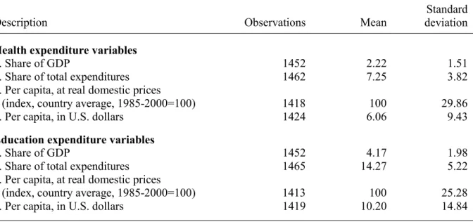
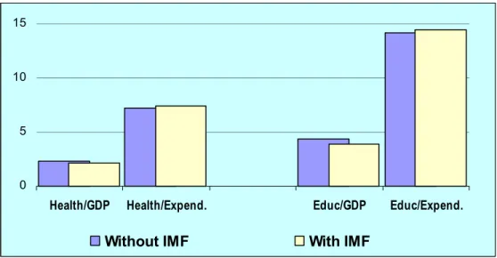
There is considerable variation in the amount of resources that developing countries devote to public expenditures on health and education. Table 1 summarizes public spending levels on health and education measured in four possible ways: per capita (in U.S. dollars and in local currency units at constant prices), as a share of total public expenditures, and as a percentage of GDP. Figure 1 compares averages in these indicators for two groups: country/years when there is an IMF program (“with IMF”) and the rest (“without IMF”).9, 10The averages for the two groups are very close—the “with IMF” group being slightly lower when social spending is measured as share of GDP, and slightly higher when measured as a share of total government expenditures.
Table 1. Social Expenditure Variables (Indicators) Used in the Study
Description Observations Mean
Standard deviation
Health expenditure variables
1. Share of GDP 1452 2.22 1.51
2. Share of total expenditures 1462 7.25 3.82
3. Per capita, at real domestic prices
(index, country average, 1985-2000=100) 1418 100 29.86
4. Per capita, in U.S. dollars 1424 6.06 9.43
Education expenditure variables
5. Share of GDP 1452 4.17 1.98
6. Share of total expenditures 1465 14.27 5.22
7. Per capita, at real domestic prices
(index, country average, 1985-2000=100) 1413 100 25.28
8. Per capita, in U.S. dollars 1419 10.20 14.84
Source: IMF, Fiscal Affairs Department.
9 Years with only part of a program are allocated to each group in proportion to the length of the period under each of the two conditions. E.g, if country X embarked on an IMF program in September 1, 1990, social spending in 1990 is included in the with and without groups with weights ¼ and ¾, respectively. Similarly, in the regression analysis, the IMF variable is defined as the share of the year under a Fund program.
10 To make all indicators fit in the same scale, the figure shows the index at constant domestic prices divided by 100; i.e. the average for the 1985–2000 is set to 1.0, instead of 100 as in Table 1 and subsequent regressions.
Figure 1. Average Social Spending “With” and “Without” the IMF (1985–2000) (In percent) 0 5 10 15
Health/GDP Health/Expend. Educ/GDP Educ/Expend.
Without IMF With IMF
Source: IMF, Fiscal Affairs Department
This comparison of averages (Figure 1) provides an initial description of levels of social spending with and without IMF-supported programs; however, this information is hardly conclusive. For example, it cannot establish whether the differences depicted in the figure are (statistically) “significant.” Do the different levels of spending reflect fundamental
differences associated with the presence of a IMF-Supported program? Or are they just random fluctuations for the particular sample of countries and periods representing each group? In other words, to the extent that other factors that may also affect spending are not controlled for, the observed differences could be spuriously associated with the IMF-Supported program.11 What is needed, therefore, is a more explicit statistical analysis, including controls for those variables which may influence social spending and that are simultaneously associated with the presence of an IMF arrangement. Before embarking on this analysis, we present some results from comparing periods with and without Fund program for each particular country, where the need for control variables is somewhat less pressing.12
11 For example, IMF-supported programs are more prevalent in lower income countries (the average income per capita in the “with IMF” group is US$934, about one-third that of the “without IMF” group, US$2,722 which also spend less on health and education in U.S. dollars per capita, so it is not surprising that average social spending in U.S. dollars is smaller in the “with IMF” group.
12 Ideally, it would have been better to start by running individual country regressions (in a fully specified model with all the theoretically relevant variables) for each country in the sample. Unfortunately, the data set covers a limited time period (T=15). Hence, there is a
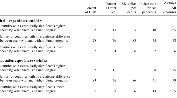
Table 2 summarizes the results for the 92–94 countries for which there is enough data to compare periods with and without a IMF-Supported program. In the majority of cases there is no statistically significant difference between both periods.13 Among the cases where there is a significant difference, the measures in shares of GDP or of total public expenditures show a majority of countries with higher education and health spending when there is a IMF-Supported program, but a majority with lower spending in terms of U.S. dollars per capita. At constant domestic prices, more countries show higher health expenditures and lower education expenditures with an IMF program.
Table 2. Summary of Country Regression Results by Significance of Measures of Social Spending
Percent of GDP Percent of total Exp. U.S. dollar per capita In domestic prices per capita Average All measures
Health expenditure variables
Countries with (statistically significant) higher
spending when there is a Fund Program. 8 13 3 10 8.5 Number of countries with no significant difference
between years with and without Fund programs 78 76 83 75 78 Countries with (statistically significant) lower
spending when there is a Fund Program. 7 4 6 7 6
Education expenditure variables
Countries with (statistically significant) higher
spending when there is a Fund Program. 7 11 1 8 6.75 Number of countries with no significant difference
between years with and without Fund programs 83 76 86 71 79 Countries with (statistically significant) lower
spending when there is a Fund Program. 5 8 6 14 8.25
Table 2 thus indicates that in most countries (about 85 percent) there is no preponderance of evidence to show that social spending levels are systematically higher or lower during periods with IMF-Supported programs. And even in the cases where the results are significant, the evidence would be stronger if it were possible to control for other factors which might correlate with periods under an IMF arrangement. As discussed in the next very small number of degrees of freedom for running individual country regressions, which would make it very difficult to obtain robust results. The alternative of running the
regressions without controls is, to be sure, also problematic. Yet, it is sufficient for our initial purpose of providing some simple initial results on the basis of intra-country comparisons. 13 At at least a 90 percent confidence level.
section, this cannot be done properly with the limited number of observations available within each country.
One possible solution to the limitations of the country by country analysis is to combine time series (observations of one unit of analysis at different points in time) with cross section data (observations of a number of units of analysis at the same point in time).14 This would help us draw some empirical conclusions about what is likely to happen to social spending for an “average” country with a IMF-Supported program.
III. THE IMPACT OF IMF-SUPPORTED PROGRAMS ON SOCIAL SPENDING:ATIME-SERIES
CROSS-SECTION ANALYSIS
Initial issues
To estimate the impact of the presence of an IMF-supported program on social spending, we need to address three potential sources of bias:
(a) Missing variables. It is necessary to include variables that have an independent effect on
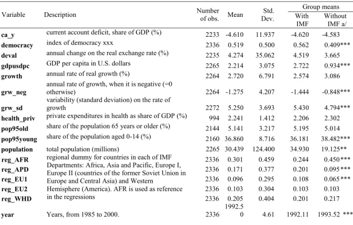
spending and that may also be associated with the presence of an IMF-supported program. Failure to do so would attribute to the presence of a Fund program, effects that are really the product of these other variables.15 The following control variables were defined using data from the World Bank’s World Development Indicators and the IMF’s World Economic
Outlook (see Table A1 in the Appendix for the summary statistics, including means for the
“with IMF” and “without IMF” groups):16
14 This method of aggregating data has two important advantages. First, it produces a relatively large N. Hence, it overcomes the “degrees of freedom” problem that typically affects individual country regressions. This allows the analyst to test for the effect of a large number of independent variables. Second, it pays attention to both longitudinal and cross-sectional variations, and can therefore produce useful generalizations across both time and space. However, the method also relies on rather stringent assumptions (e.g. parameter heterogeneity) and can potentially suffer the combined pitfalls of cross-sectional analysis (e.g. heteroskedasticity) and time-series analysis (e.g. nonstationarity, serial correlation, etc.) 15 “Omitted variables” bias is one of the most serious problems in econometrics. Unlike other problems such as heteroskedasticity, multicollinearity or serial correlation (without a lagged endogenous variable), omitting relevant variables leads to biased and inconsistent parameter estimates.
16 Two of the control variables (health_priv and ca_y) had insignificant coefficients and were excluded from the final regressions.
gdpusdpc = GDP per capita in U.S. dollars
health_priv = private expenditures in health as share of GDP (percent) pop95young = share of the population aged 0–14 (percent)
pop95old = share of the population 65 years or older (percent) growth = annual rate of real growth (percent)
grw_neg = annual rate of growth, when it is negative (=0 otherwise) grw_sd = variability (standard deviation) on the rate of growth ca_y = current account deficit, share of GDP (percent) devaluation = annual change on the real exchange rate (percent) democracy = index of democracy from the Polity IV dataset17
The above control variables are important in accounting for the differences in social spending levels among countries. We discuss briefly the expected impact of some of these variables. First, we follow most empirical studies of the welfare state by including a measure of economic development to control for Wagner’s Law, according to which industrialization and modernization lead to an expansion of public activity over private activity. This occurs because in an increasingly complex society, the need for expenditures on regulatory activities grows. In addition, the demand for collective or quasi-collective goods—in particular
education and culture—tends to be income elastic (i.e. its demand increases as income grows). As a result, as countries become wealthier, the state has to increase its supply of these goods, which would otherwise be undersupplied by the market.18 Second, our model also includes three measures of changes in output levels (i.e. the annual rate of real GDP growth, a dummy for years of negative GDP growth, and a measure of output volatility) that are likely to affect the amount of resources that countries can devote to social spending. Finally, we also include a variable that measures “democracy” using a numerical scale. The scale measures the degree to which elections are free and fair and basic civil rights and liberties are respected by the state. Democracy is expected to have a positive impact on social expenditures for two reasons: (a) in a democratic regime political leaders are more dependent on the popular vote and, to the extent that social expenditures can be used to gain the support of important electoral constituencies, politicians are more likely to increase the resources they allocate to the social sector; and (b) democratic regimes tend to have better developed civil societies that can more effectively press the state for social protection.
17 The index is defined from Gurr’s AUTOC and DEMOC scores: democracy=1 when DEMOC–AUTOC > 4, following Brown and Hunter (1999). See also Kaufman and Segura-Ubiergo (2001).
18 Another possible analytic framework to study the relationship between economic development and the size of the public sector is Baumol’s cost disease (See for example Baumol, 1993). According to Baumol, real wages in the private and public sectors grow at roughly the same rate. However, because the public sector is labor-intensive and mainly service-oriented, productivity in this sector in fact grows at a lower rate than in the private sector. Hence, the relative size of government in the economy grows.
These control variables can help explain some of the differences in spending between
countries, but there may be residual country differences in spending not captured by them. To account for this possibility, the empirical model was also estimated with fixed effects, which allow for a different level of average spending for each country.19
(ii) Serial correlation and nonstationarity. Spending on social services tends to change
sluggishly and be heavily affected by the level of spending during previous periods. This reflects not only the fact that most programs are often conceived as permanent or at least spanning several years, but also the political economy of budget allocation in which most programs have constituencies who resist change. For these reasons, changes in control variables (and IMF-supported programs) are likely to have an impact which is not instantaneous and may extend beyond one period. Thus, the empirical analysis should
include a richer dynamics that distinguishes between short and medium term effects on social expenditures.
The empirical analysis addressed this issue by including the following:
• The value of social spending in the previous year (lagged y, or LY), to account for the dependence of current spending on past allocations.
• The value of all control variables in the previous period (LX), as well as the change (difference) between current and previous period values (DX). This permits each control variable to have either just a transitory effect on the current period (variable
DX), or an extended effect over several periods.
• Similar specification for the presence of a Fund program (lagged and difference:
LIMF and DIMF), which allows for a richer dynamic on the impact of these programs.
The above variables were then combined in an Autoregressive Moving Average process (ARIMA) which was sufficient to obtain independent and identically distributed residuals (IID). The structural equation of the ARIMA process is given by
[2] Sit = γLSi,t + LXit α0 + DXit α1 + β0LIMFit + β1DIMFit + uit
where L is the lag operator (i.e., LZt≡ Zt-1, for any variable Z), D is the first-difference operator (D Zt ≡ Zt – Zt-1), and uit are the new independent and identically distributed residuals (IID), which are not affected by serial correlation. In order to disentangle short and medium-term effects, it is useful for analytical purposes to rewrite equation 2 as
[2a] DSit = DXit α1 + β1DIMFit + (1 – γ )( LXit α2 + LIMFit β2 – LSit) + uit
where (1 – γ )α2 = α1 and (1 – γ )β2 = β1. In this specification, changes in the dependent variables, DSit , can be seen as the result of two effects: contemporaneous changes in the explanatory variables (with an impact determined by the coefficients α1 and β1 ); and gradual adjustment to an “equilibrium” level of spending, determined by the coefficients α2 and β2). Transitory changes in the independent variables do not change the long run “equilibrium” level, so that the effect decays geometrically at the rate (1 – γ) after the second period
(iii) Endogeneity of Fund programs. Countries only engage the Fund and agree to its
monitoring when they have an urgent need to access the resources that it provides. Thus, years with a IMF-supported program are not “normal” years. The special factors leading to the presence of a program could also, in principle, have an independent impact on social expenditures. For example, a country could seek a Fund program as result of an external crisis (e.g. a large increase in the price of imports or a fall in export prices), and such a crisis is likely to require a reduction in government expenditures with or without the Fund.20 To address this issue, the following instruments were used to “predict” the presence of a program:
• Current account deficit as fraction of GDP in the previous year (as proxy of external crisis).
• Growth in the previous year (proxy of unsustainable expansion?).
• Income per capita (IMF-supported programs less likely on high income countries).
• Presence of a Fund program in the previous year.
• Government balance as share of GDP in the previous year.
• Democracy index (as in the control variables).
20 In the absence of any rigorous way of defining counterfactuals (i.e. deciding what would have been the level of government social expenditures under a given set of conditions with
and without a Fund program), the standard way to improve the estimation of the coefficients
of endogenous variables is to estimate these variable together with the original equation. As the main interest is in the spending equations, though, we do not need a full estimation of the likelihood of an IMF program: it is enough to estimate the regression using instrumental variables. It is also not critical to include all the determinants of the IMF variable, provided that the set of instrumental variables at least includes all the factors which potentially affect both, the presence of a program and the level of social spending, since these are the factors that biased the estimate of the IMF variable.
IV. RESULTS
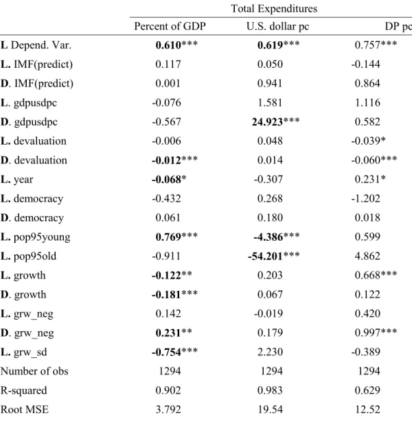
Table 3 presents regression results for the eight definitions of social spending, four for education and four for health. All eight indicators of health andeducation expenditures show positive coefficients for the contemporaneous and lagged values of the IMF variable; only three of the 16 coefficients are not significantly different from zero at least at a 90 percent confidence level (i.e. *, **, *** represent the 90, 95, and 99 percent confidence intervals), and 5 are significant at 99 percent level. It is interesting that this seems to reflect a specific effort to protect these types of expenditures, as total public expenditures are not significantly different with a without the IMF (see Table A3 in Appendix).
Table 3. ARIMA Model with Control Variables and Endogenous Fund Programs
Health Education
GDP Total Exp. U.S. dollar pc DP pc GDP Total Exp. U.S. dollar pc DP pc (In percent) L Depend. Var. 0.577 *** 0.548 *** 0.748 *** 0.688 *** 0.604 *** 0.559 *** 0.662*** 0.743*** L.IMF(predicted) 0.179 *** 0.492 * 0.390 * 4.593 0.251 ** 0.681 * 0.168 4.157 D.IMF(predicted) 0.206 *** 0.636 ** 0.395 ** 9.736 *** 0.228 *** 0.748 ** 0.333 6.027** L.gdpusdpc -0.030 * -0.027 0.014 -0.164 0.021 0.070 0.517 1.406 D.gdpusdpc -0.080 *** -0.093 1.101 *** -2.761 ** -0.034 0.125 2.144*** 0.178 L.devaluation 0.002 ** 0.012 *** 0.010 *** 0.109 *** -0.001 0.001 0.011*** 0.007 D.devaluation 0.001 0.008 *** 0.005 *** 0.046 * -0.001 0.000 0.005** -0.025 L.year 0.011 *** 0.068 *** -0.002 1.219 *** 0.012 * 0.104 *** -0.012 0.686*** L.democracy 0.061 0.342 0.221 * 2.917 0.142 0.620 * 0.114 4.969 D.democracy 0.009 0.308 0.072 1.784 0.035 0.428 0.056 2.852 L.pop95young -0.031 ** -0.015 -0.190 0.059 0.023 0.211 *** -0.190 1.593*** L.pop95old -0.129 * -0.120 -1.980 *** -1.528 -0.116 -0.119 -3.745*** 3.560 L.growth 0.013 * 0.028 0.073 ** 1.521 *** -0.010 -0.047 0.050 0.779*** D.growth 0.005 0.019 0.033 0.895 *** -0.021 *** -0.035 0.025 0.320 L.grw_neg -0.049 *** -0.060 -0.078 * -1.736 *** -0.024 0.022 -0.045 -0.399 D.grw_neg -0.035 ** -0.025 0.000 -1.027 ** 0.004 0.036 0.060 0.236 L.grw_sd 0.047 *** 0.000 0.386 *** -0.029 0.050 ** -0.118 0.955*** -0.831* Number of obs 992 1001 992 992 989 1001 989 989 R-squared 0.931 0.894 0.985 0.544 0.918 0.881 0.987 0.626 Root MSE 0.408 1.375 1.209 20.569 0.597 1.952 1.761 15.591
Note: See the text for variable definitions. An initial L indicates a lagged value and D the first difference. IMF(predict) is the estimated value of the IMF variable with the following instruments: lagged values of IMF, growth, CA/GDP, Government Balance/GDP, Democracy index and GDP per capita in U.S. dollars (pc= per capita and DP= domestic prices) . The actual estimated equation is.
IMF(predicted) = 0.148 + 0.696 IMF(-1) - 0.003 growth(-1) + 0.001 ca_y(-1)+ 0.001.cgbal(-1) – 0.043 democracy -0.011.gdpusdpc; N=1916 (41.94***) (-2.58***) (-0.69) (0.60) (-3.26***) (-4.85***) R2 = 0.522
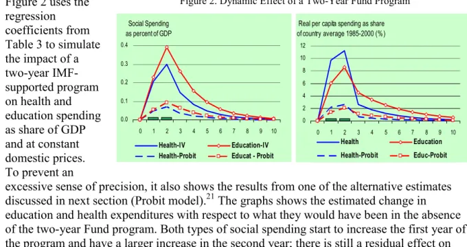
Figure 2. Dynamic Effect of a Two-Year Fund Program Social Spending as percent of GDP 0.0 0.1 0.2 0.3 0.4 0 1 2 3 4 5 6 7 8 9 10 Health-IV Education-IV
Health-Probit Educat - Probit
Real per capita spending as share of country average 1985-2000 (%) 0 2 4 6 8 10 12 0 1 2 3 4 5 6 7 8 9 10 Health Education Health-Probit Educ-Probit
Figure 2 uses the regression coefficients from Table 3 to simulate the impact of a two-year IMF-supported program on health and education spending as share of GDP and at constant domestic prices. To prevent an
excessive sense of precision, it also shows the results from one of the alternative estimates discussed in next section (Probit model).21 The graphs shows the estimated change in education and health expenditures with respect to what they would have been in the absence of the two-year Fund program. Both types of social spending start to increase the first year of the program and have a larger increase in the second year; there is still a residual effect on the third year (i.e. after the end of the program), which declines geometrically at about 40 percent a year from then on.
The results of Table 3 stand in contrast with the ambiguous results for the group means in Figure 1 and the country time series reported in Table 2. Thus, it is particularly important to explore their robustness with respect to the estimation methodology and the country sample. This is the task of the next section.
V. ROBUSTNESS OF THE RESULTS.
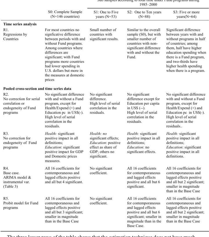
Table 4 summarizes the results of sensitivity analysis.22 Specifically, we consider the following alternatives:
• Estimation methodology:
1. No correction for serial correlation or endogeneity of Fund programs. 2. Correction for Serial Correlation but not for endogenous Fund programs.
21 A probit model differs from the Instrumental Variables (IV) estimate used in Table 3 in explicitly constraining the predicted IMF variable to values between zero and one.
3. Alternative correction for endogenous programs, to take into account that the proportion of the year under a program must be between zero and one (Probit model).
• Sub samples of countries:
S1. Excluding nonusers and moderate users: includes countries with at least one
year but no more than six years of Fund programs
S2. Excluding non-users and chronic users: includes countries with at least one
year but no more than ten years of Fund programs
S3. Only repeat users: includes countries with five or more years of IMF
programs.
By comparing alternative estimation techniques, i.e. different rows of Table 4, we see that the first two rows do not produce any strong conclusion about the impact of Fund programs on spending: either the coefficients are not significant or the number of positive coefficients are roughly on balance with the negative ones. There are, however, interesting differences in the four sub samples results shown in the first row, comparing spending with and without the Fund for each country separately. Among countries with five or more years of programs there is a much larger proportion of countries in which social spending are higher in years with programs. A more detailed analysis would be needed to evaluate hypothesis of why this is the case.23 But these “repeat users” do have significant influence in the results.
23 E.g. it could be that those countries which are frequent clients are more prone to crisis, which could have a negative impact on social spending.
Table 4. Summary of Robustness Analysis
Sub samples according to total time under Fund programs during 1985–2000
S0: Complete Sample
(N=146 countries) S1: One to Five years (N=53)
S2: One to Ten years (N=88)
S3: Five or more years(N=64)
Time series analysis
R1.
Regressions by Countries
For most countries no signficative difference between periods with and without Fund programs. Among countries where differences are significant; with Fund programs more countries had lower spending in U.S. dollars but more in the measures at domestic prices
Small number of countries with significant results.
Similar to the overall sample (S0), but with smaller number of countries with non-significant difference with and without the Fund.
Significant difference between years with and without programs in half of countries; among them, half have higher education spending when there is a Fund program, and two-thirds have higher health spending when there is a program.
Pooled cross-section and time series data
R2.
No correction for serial correlation or
endogeneity of Fund programs
No significant difference with and without a Fund program, except for Health/Expend (+) and Education pc in US$(-). High level of serial correlation in the residuals.
No significant difference. High level of serial correlation in the residuals.
No significant difference except for Education per capita in US$ (--). High level of serial correlation in the residuals.
No significant difference with and without a Fund program, except for Health/Expend (+) and Education pc in US$(-). High level of serial correlation in the residuals.. R3. No correction for endogeneity of Fund programs Health: significant positive impact in all definitions;
Education: significant positive impact for GDP and Domestic prices measures. Health: no significant effects; Education: positive effect as share of GDP; others no significant. Health: significant positive impact in all definitions;
Education: no significant effects.
Health: significant positive impact in all definitions;
Education: significant positive impact in all definitions.
R4. Base case. ARIMA model & instrumental var. (Table 3)
All 16 coefficients for contemporaneous and lagged effects positive and all but 4 significant.
No significant coefficient.
All 16 coefficients for contemporaneous and lagged effects positive and all but 6 significant.
All 16 coefficients for contemporaneous and lagged effects positive and all but 2 significant; smaller in magnitude than in the Base Case R5.
Probit model for Fund programs
All 16 coefficients for contemporaneous and lagged effects positive and all but 3 significant; smaller in magnitude than in the Base Case
No significant coefficient.
All 16 coefficients for contemporaneous and lagged effects positive and all but 6 significant; smaller in magnitude than in the Base Case.
All 16 coefficients for contemporaneous and lagged effects positive and all but 2 significant; smaller in magnitude than in the Base Case
The three lower rows of the table shows that the estimation technique does not have much effect on the qualitative results about the impact of Fund programs (the magnitude of the impact does change, as already illustrated in Figure 2).
VI. CONCLUSIONS
This paper has argued that the popular view of the IMF leading to dramatic declines of social spending is not borne out by the available empirical evidence. In fact, the presence of an IMF-supported program tends to either maintain or increase social spending in health and education, measured as either a share of GDP, total expenditures or in real per capita terms. The effect is relatively small and short-lived and particularly significant for countries which are continuing (but not necessarily chronic) clients of the IMF. We found no significant difference between concessional and non-concessional programs. However, our analysis did not include indicators of actual health or educational outcomes. Hence, we presented no evidence of whether the programs affect the efficiency of delivery of those services or their targeting.
Our paper suggests three areas for further research. First, ours is the first attempt we know of to measure the impact of an IMF-supported program on social expenditure using an
econometric model. Measuring the impact of the IMF is a very difficult task given the existence of a number or well-known statistical problems (e.g. endogeneity of Fund
programs, parameter heterogeneity, serial correlation and unit roots, panel heteroskedasticity, etc.). Although we have been careful to test for the robustness of our results in a number of ways, given the number of potential methodological pitfalls that may affect the study of the impact of IMF-supported programs, the evidence we present can only be taken as tentative. Researchers that have attempted to measure the impact of the IMF on key macroeconomic variables (e.g. growth, the current account, inflation) often get contradictory results that are sensitive to the methodological choices they make. Hence, our evidence only leads to tentative conclusions. Much more analytical and empirical work is needed to evaluate more precisely the impact of IMF-supported programs on social spending.
Second, the main limitation of our study is that it does not allow us to draw any conclusions about the impact of IMF-supported programs on the poor. As noted, social expenditures in developing countries vary enormously in terms of their equity, efficiency and sustainability. One obvious task for further research would be to try to unbundle the direct and indirect impact of IMF-supported programs on the poor using social expenditures as an intervening variable. For example, even if IMF-supported programs managed to maintain constant (or increase slightly) social expenditures during times of budgetary retrenchment, this might not be particularly helpful to protect the poor if expenditures on wages and salaries “crowd out” expenditures on goods and services that more directly benefit the poor. On the other hand, even if social expenditure levels declined, this might not lead to worse poverty indicators if the efficiency or targeting of expenditures increased.
Finally, like all statistical studies, our analysis can point to associations among variables but cannot establish with precision what are the causal mechanisms at work. Hence, another useful way to expand our research would be to draw evidence from in-depth case studies where the transmission mechanisms between the presence of an IMF-supported program, social expenditures and poverty outcomes can be more effectively and convincingly established.
BIBLIOGRAPHY
Abed, George T., Liam Ebrill, Sanjeev Gupta, Benedict Clemens, Ronald McMorran, Anthony Pellechio, Jerald Schiff, and Marijn Verhoeven, 1998, “Fiscal Reforms in Low-Income Countries,” IMF Occasional Paper No. 160 (Washington: International Monetary Fund).
Bagci, Pinar and William Perraudin,1997, “The Impact of IMF Programmes,” Global
Economic Institutions Working Paper, No. 24.
Baqir, Reza, 2002, “Social Sector Spending in a Panel of Countries,” IMF Working Paper
02/35, February (Washington: International Monetary Fund).
Barro, Robert J. and Jong-Wha Lee, 2002, “IMF Programs: Who is Chosen and What are the Effects?” NBER Working Paper 8951 (Cambridge, MA: National Bureau of
Economic Research).
Baltagi, Badi and Qi Li, 2002, “On instrumental variable estimation of semiparametric dynamic panel data models,” Economic Letters 76: 1–9.
Banerjee, Anindya., Juan Dolado, John Galbraith, and David Henry, 1993, Co-Integration,
Error Correction, and the Econometric Analysis of Nonstationary Data (Oxford:
Oxford University Press).
Baumol, William, J., 1993, “Healthcare, Education and Cost Disease—A Looming Crisis for Public Choice,” Public Choice, 77:17–28.
Bird, Graham and Dane Rowlands,1997, “The Catalytic Effect of Lending by the International Institutions,” World Economy Vol. 20(7): 967–991.
Brown, David S. and Wendy Hunter, 1999, “Democracy and Social Spending in Latin America, 1980-92,” American Political Science Review, 93(4): 779–790. Bretton Woods Project, 2004, “The World Bank and IMF at Sixty” at
http://www.brettonwoodsproject.org.
Bulir, Ales and Soojin Moon, 2003, “Do IMF-Supported Programs Help Make Fiscal Adjustment More Durable,” IMF Working Paper 03/38 (Washington: International Monetary Fund).
Conway, Patrick, 1994, “IMF Lending Programs: Participation and Impact,” Journal of
Development Economics 45(2): 365–91.
Dicks-Mireaux, Louis, Mauro Mecagni and Susan Schadler, 2000, “Evaluating the Effect of IMF lending to low income countries,” Journal of Development Economics 61: 495-526.
Dollar, David and Jakob Svensson, 2000, “What Explains the Success or Failure of Structural Adjustment Programmes?” Economic Journal 110: 894–917.
Ergin, Evren (1999) “Determinants and Consequences of International Monetary Fund Programs,” PhD Dissertation, Stanford University.
Hahn Jinyong and Jerry Hausman, 2002, “A new specification test for the validity of instrumental variables,” Econometrica 70(1): 163–189.
Joyce, Joseph P., 2002, “Through a Glass Darkly: What We Know (and Don’t Know) about IMF Programs,” Wellesley College Working Paper 2002-04, June.
Garuda, G.,2000, “The Distributional Effects of IMF Programs: A Cross-Country Analysis,”
World Development, Vol.28(6): 1031–1051.
Global Exchange, 2001, “How the International Monetary Fund and the World Bank Undermine Democracy and Erode Human Rights—Five Case Studies”. Available at
http://www.globalexchange.org/campaigns/wbimf/wbimfReport.pdf
Goldstein, Morris, and Peter Montiel, 1985, “Evaluating Fund Stabilization Programs with Multicountry Data: Some Methodological Pitfalls,” IMF Staff Papers 33(2): 304–344. Greene, William, 2000, Econometric Analysis (New Jersey: Prentice Hall).
Gupta, Sanjeev, Benedict Clements and Erwin Tiongson, 1998, “Public Spending on Human Development,” Finance & Development, September.
Gupta, Sanjeev, Benedict Clemens, Maria Teresa Guin-Siu, and Luc Leruth, 2001, “Debt Relief and Public Health Spending in Heavily Indebted Poor Countries,” Finance &
Development Vol. 38 (3): pp. 10–13
Gupta, Sanjeev, Louis Dicks-Mireaux, Ritha Khemani, Calvin McDonald, and Marijn Verhoeven, 2000, “Social Issues in IMF-Supported Programs,” IMF Occasional
Paper No. 191 (Washington: International Monetary Fund).
Haque, Nadeem Ul and Mohsin S. Khan, 1998, “Do IMF-Supported Programs Work? A Survey of Cross-Country Empirical Evidence,” IMF Working Paper No. 98/169 (Washington: International Monetary Fund).
Heller, Peter, A. Lans Bovenberg, Thanos Catsambas, Ke-Young Chu, and Parthasarathi Shome, 1988, “The Implications of IMF-Supported Programs for Poverty. Experiences in Selected Countries,” Occasional Paper No. 58 (Washington: International Monetary Fund)
International Monetary Fund, 1998, “The IMF and the Poor,” Pamplet No. 52, Fiscal Affrairs Department (Washington: International Monetary Fund).
Kaufman, Robert and Alex Segura-Ubiergo, 2001, “Globalization, Domestic Politics and Social Spending in Latin America: A Time-Series Cross-Section Analysis” World
Politics 53 (4): 553–87.
Khan, Mohsin, 1990, “The Macroeconomic Effects of IMF-Supported Programs,” IMF Staff
Papers 37(2):1-23.
Kmenta, Jan, 1997, “Elements of Econometrics,” (Ann Arbor: University of Michigan Press). Mackenzie, G.A., David W.H. Orsmond, and Philip R. Gerson, 1997, “The Composition of
Fiscal Adjustment and Growth. Lessons from Fiscal Reforms in Eight Economies,”
IMF Occassional Paper No. 149 (Washington: International Monetary Fund).
Naiman, Robert and Neil Watkins, 1999, “A Survey of the Impacts of IMF Structural Adjustment in Africa: Growth, Social Spending and Debt Relief”, Report, April (Washington: Center for Economic and Policy Research).
Przeworski, Adam and James Vreeland, 2000, “The Effects of IMF Programs on Economic Growth”. Journal of Development Economics 62: 385–421.
Rodrik, Dani,1996, “Why is There Multilateral Lending? In Bruno, M and Pleskovic, B (eds.),” Annual World Bank Coference on Development Economics 1995. pp. 167-193 (Washington; World Bank).
Table A1. Summary Statistics for the Control Variables for Social Spending
Group means Variable Description Number of obs. Mean Dev.Std. With
IMF
Without IMF a/
ca_y current account deficit, share of GDP (%) 2233 -4.610 11.937 -4.620 -4.583
democracy index of democracy xxx 2336 0.519 0.500 0.562 0.409***
deval annual change on the real exchange rate (%) 2235 4.274 35.062 4.519 3.665
gdpusdpc GDP per capita in U.S. dollars 2265 2.214 3.075 2.722 0.934***
growth annual rate of real growth (%) 2264 2.720 6.791 2.574 3.086
grw_neg
annual rate of growth, when it is negative (=0
otherwise) 2264 -1.275 4.207 -1.444 -0.848***
grw_sd
variability (standard deviation) on the rate of
growth 2272 5.250 3.693 5.430 4.794***
health_priv private expenditures in health as share of GDP (%) 994 2.241 1.412 2.206 2.302
pop95old share of the population 65 years or older (%) 2144 5.141 3.217 5.195 5.014
pop95young share of the population aged 0-14 (%) 2160 36.860 8.716 36.181 38.482***
population total population (millions) 2265 30.439 124.400 34.930 19.125**
reg_AFR 2336 0.301 0.459 0.244 0.450***
reg_APD 2336 0.171 0.377 0.201 0.095***
reg_EU1 2336 0.096 0.295 0.108 0.065***
reg_EU2 2336 0.103 0.304 0.103 0.103
reg_WHD
regional dummy for countries in each of IMF Departments: Africa, Asia and Pacific, Europe I, Europe II (countries of the former Soviet Union in Europe and Central Asia) and Western
Hemisphere (America). AFR is used as reference
in the regressions 2336 0.205 0.404 0.201 0.217
year Years, from 1985 to 2000. 2336 1992.50 4.61 1992.11 1993.52 ***
Note
Table A2. IMF-Supported Programs and Total Public Spending.
Total Expenditures
Percent of GDP U.S. dollar pc DP pc
L Depend. Var. 0.610*** 0.619*** 0.757*** L. IMF(predict) 0.117 0.050 -0.144 D. IMF(predict) 0.001 0.941 0.864 L. gdpusdpc -0.076 1.581 1.116 D. gdpusdpc -0.567 24.923*** 0.582 L. devaluation -0.006 0.048 -0.039* D. devaluation -0.012*** 0.014 -0.060*** L. year -0.068* -0.307 0.231* L. democracy -0.432 0.268 -1.202 D. democracy 0.061 0.180 0.018 L. pop95young 0.769*** -4.386*** 0.599 L. pop95old -0.911 -54.201*** 4.862 L. growth -0.122** 0.203 0.668*** D. growth -0.181*** 0.067 0.122 L. grw_neg 0.142 -0.019 0.420 D. grw_neg 0.231** 0.179 0.997*** L. grw_sd -0.754*** 2.230 -0.389 Number of obs 1294 1294 1294 R-squared 0.902 0.983 0.629 Root MSE 3.792 19.54 12.52
Note: a/ Statistically significant differences in means are indicated by *** (99 percent confidence level) or **(95percent).
Table A3. List of Countries and Sub samples Years Country IMF S1 S2 S3 Albania 5.71 S1 S2 S3 Algeria 4.81 S1 S2 Angola 0.00 Argentina 11.76 S3 Armenia 4.48 S1 S2 Azerbaijan 4.13 S1 S2 Bahamas, The 0.00 Bahrain 0.00 Bangladesh 6.59 S1 S3 Barbados 1.31 S1 S2 Belarus 1.00 S1 S2 Belize 1.24 S1 S2 Benin 9.61 S1 S3 Bhutan 0.00 Bolivia 12.10 S3
Bosnia & Herzegovina 1.00
Botswana 0.00 Brazil 6.35 S1 S3 Bulgaria 7.34 S1 S3 Burkina Faso 9.77 S1 S3 Burundi 5.26 S1 S2 S3 Cambodia 3.56 S1 S2 Cameroon 7.86 S1 S3 Cape Verde 1.16 S1 S2
Central African Republic 2.45 S1 S2
Chad 8.23 S1 S3
Chile 3.02 S1 S2
China 0.00
Colombia 1.03 S1 S2
Comoros 2.45 S1 S2
Congo, Dem. Rep. Of 4.42 S1 S2
Congo, Republic of 5.41 S1 S2 S3 Costa Rica 6.59 S1 S3 Cote d’Ivoire 10.94 S3 Croatia 4.50 S1 S2 Cyprus 0.00 Czech Republic 1.00 Djibouti 2.37 S1 S2 Dominica Dominican Republic Ecuador Egypt El Salvador Equatorial Guinea Eritrea Estonia Ethiopia Fiji Gabon 9.20 S1 S3 Gambia, The 8.55 S1 S3 Georgia 4.08 S1 S2
Table A3. List of Countries and Sub samples Years Country IMF S1 S2 S3 Ghana 11.78 S3 Grenada 1.64 S1 S2 Guatemala 2.59 S1 S2 Guinea 13.38 S3 Guinea Bissau 0.00 Guyana 10.12 S3 Honduras 6.29 S1 S3 Hungary 7.75 S1 S3 India 1.66 S1 S2 Indonesia 3.16 S1 S2 Iran 0.00 Jamaica 9.73 S1 S3 Jordan 9.42 S1 S3 Kazakhstan 6.05 S1 S3 Kenya 6.99 S1 S3 Kiribati 0.00 Korea 4.90 S1 S2 Kuwait 0.00 Kyrgyz Republic 7.12 S1 S3 Lao PDR 6.63 S1 S3 Latvia 7.13 S1 S3 Lebanon 0.00 Lesotho 8.72 S1 S3 Liberia 1.43 S1 S2 Libya 0.00 Lithuania 5.74 S1 S2 S3 Macedonia FYR 3.41 S1 S2 Madagascar 9.63 S1 S3 Malawi 10.13 S3 Malaysia 0.00 Maldives 0.00 Mali 13.38 S3 Malta 0.00 Marshall Islands 0.00 Mauritania 12.16 S3 Mauritius 1.50 S1 S2 Mexico 8.30 S1 S3 Moldova 5.29 S1 S2 S3 Mongolia 6.29 S1 S3 Morocco 5.95 S1 S2 S3 Mozambique 10.52 S3 Myanmar 0.00 Namibia 0.00 Nepal 6.24 S1 S3 Netherlands Antilles 0.00 Nicaragua 4.99 S1 S2 Niger 10.96 S3 Nigeria 3.90 S1 S2 Oman 0.00 Panama 7.93 S1 S3
Table A3. List of Countries and Sub samples Years Country IMF S1 S2 S3 Paraguay 0.00 Peru 8.27 S1 S3 Philippines 11.92 S3 Poland 5.83 S1 S2 S3 Qatar 0.00 Romania 5.15 S1 S2 S3 Russia 5.37 S1 S2 S3 Rwanda 5.13 S1 S2 S3 Samoa 0.52
Sao Tome & Principe 3.18 S1 S2
Saudi Arabia 0.00 Senegal 13.93 S3 Seychelles 0.00 Sierra Leone 6.87 S1 S3 Slovak Republic 1.67 S1 S2 Solomon 0.00 South Africa 0.00 Sri Lanka 6.27 S1 S3
St. Kitts and Nevis 0.00
St. Lucia 0.00 Suriname 0.00 Swaziland 0.00 Syria 0.00 Tajikistan 3.18 S1 S2 Tanzania 10.09 S3 Thailand 4.63 S1 S2 Togo 12.07 S3 Tonga 0.00
Trinidad & Tobago 2.07 S1 S2
Tunisia 4.49 S1 S2
Turkey 2.45 S1 S2
Turkmenistan 0.00
Uganda 11.66 S3
Ukraine 5.08 S1 S2 S3
United Arab Emirates 0.00
Uruguay 8.47 S1 S3
Uzbekistan 1.24 S1 S2
Vanuatu 0.00
Venezuela 4.00 S1 S2
Vietnam 3.30 S1 S2
Vincent & the Grenadines 0.00
Yemen 4.60 S1 S2
Zambia 7.48 S1 S3