Report no. 10/5
A general framework for solving Riemann–Hilbert problems
numerically
Sheehan Olver
Abstract A new, numerical framework for the approximation of solutions to matrix-valued Riemann–Hilbert problems is developed, based on a recent method for the homogeneous Painlev´e II Riemann–Hilbert problem. We demonstrate its effectiveness by computing solutions to other Painlev´e tran-scendents. An implementation in Mathematica is made available online.
Keywords Riemann–Hilbert problems, singular integral equations, colloca-tion methods, Painlev´e transcendents.
Oxford University Mathematical Institute Numerical Analysis Group
24-29 St Giles’
Oxford, England OX1 3LB
1. Introduction
The solution to integrable, nonlinear differential equations can typically be written as Riemann–Hilbert (RH) problems. Examples include the Painlev´e I–V transcendents [8], the Korteweg-de Vries (KdV) equation and the nonlinear Schr¨odinger (NLS) equation [1]. The importance of RH problems lies in the fact that they are often solvable asymptotically, which allows one to determine the asymptotics of solutions to the corresponding differential equation. This is accomplished using nonlinear steepest descent [5], a modification of a tool which is very familiar in asymptotic analysis: the method of steepest descent. In short, they can be viewed roughly as generalizations of integral representations.
RH problems also play an increasingly crucial role in the theory of orthogonal polynomials and random matrix theory [4]. Just as in the theory of integrable systems, they are useful in the determination of asymptotics of orthogonal polynomials. But the behaviour of orthogonal polynomials is in turn directly related to the asymptotics of eigenvalues of large random matrices. This has led to new results of universality: random matrices with vastly differing behaviour have eigenvalue distributions which are the same as the dimension of the matrix becomes large.
The reduction of a problem (such as a differential equation) to an integral representation is traditionally viewed as “solving” the problem, precisely because asymptotics are then readily available. But there is another important reason why integral representations are considered solutions: they can be used for numerics as well, through quadrature. The goal of this paper is to show that RH problems can also be used for numerics. Thus, reduction of a problem to a RH problem can be viewed, in a concrete sense, as a solution to the problem. Though much research exists on numerical solution of the nonlinear RH problems used in conformal mapping [19,18,20,11]; the same is not true for the matrix-valued RH problems that are prevalent in modern applied analysis. The first use of matrix-valued RH problems as a numerical tool appears to be the thesis of Dienstfrey [6], which developed an approach for the computation of the RH problem connected with the sine kernel Fredholm determinant, of importance in random matrix theory. However, in this approach, an exponential amount of work at junction points of the domain was needed to achieve convergence, due to blow-up of the approximate solution at these points. This phenomenon was avoided in the development of an approach for the RH problem related to the homogeneous Painlev´e II equation [14], by taking the behaviour at the junction point into account.
We will generalize the latter approach in the construction of a framework applicable to a broad class of RH problems. Moreover, it could potentially provide the foundation of a toolbox for computing Painlev´e transcendents reliably. Just as RH problems are the nonlin-ear analogue of integral representations, Painlev´e transcendents can be viewed as nonlinear special functions.
I III
IV V
II
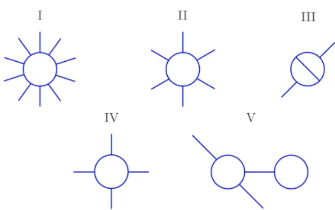
Figure 1: The jump curves for the first five Painlev´e transcendents.
2. Overview of the approach
A RH problem is a boundary value problem of finding an analytic function which satisfies a given jump condition along a curve on which analyticity is lost. More precisely:
Problem 2.1[10] Given an oriented curve Γ⊂Cand a jump matrix G: Γ→C2×2, find a function Φ :C\Γ→C2×2 which is analytic everywhere except on Γsuch that
Φ+(z) = Φ−(z)G(z) for z ∈Γ and Φ(∞) =I,
where Φ+ denotes the limit of Φ asz approaches Γ from the left, and Φ− denotes the limit of Φ asz approaches Γ from the right and Φ(∞) = lim|z|→∞Φ(z).
The jump curves Γ for the first five Painlev´e transcendents are depicted in Figure 1, cf. [8]. Note that each jump curve consists of a union of pieces conformally mappable to the unit interval: intervals, rays and arcs.
Consider the Cauchy transform (which is related to the Hilbert transform and Stieltjes transform) CΓf(z) = 1 2iπ Z Γ f(t) t−z dt.
Normally, Γ is implied byf, so we suppress the dependence and use simply C. This operator maps a H¨older-continuous functionf defined on Γ to a function which is analytic everywhere in the complex plane except on Γ, and which vanishes at ∞. Thus, as in [6,14], we write Φ =CU +I, and Problem 2.1 becomes
C+U −(C−U)G=G−I on Γ, (2.1) where C± denotes the left/right limits of the Cauchy transform. Now the operator LU =
We can use this linear operator in the construction of a collocation method. Suppose we have a sequence of pointsx= (x1, . . . , xN)> on Γ and we wish to represent the solution
by its values at these points U = (U1, . . . , UN)> (Ui are either matrices or row vectors,
but we treat them as elements in an abstract field, though what follows could be rewritten in terms of block matrices). Now if we have a scalar basis (represented as a row-vector) Ψ(z) = (ψ1(z), . . . , ψN(z)) and a transform matrix F from values at xto the coefficients of
Ψ, then, at least conceptually, we can write the collocation system as
h
C+Ψ(x)−rdiag (G)C−Ψ(x)iFU = diag (G)−I, (2.2) whereG=G(x) = (G(x1), . . . , G(xN))> and rdiag corresponds to matrix multiplication on
the right: rdiag G1 .. . GN A1 .. . AN = A1G1 .. . ANGN . To be precise, C±Ψ(x) = C±ψ1(x1) · · · C±ψN(x1) .. . . .. ... C±ψ1(xN) · · · C±ψN(xN) .
Note that the rows ofU are typically row-vectors or matrices whileC±Ψ(x) is a matrix whose entries are scalars. We treat these multiplications in the natural way: if aij are scalars and
bi are row vectors or matrices, then a11 · · · a1n .. . . .. ... an1 · · · ann b1 .. . bn = a11b1+· · ·+a1nbn .. . an1b1+· · ·+annbn
Once we have computed the values U by solving (2.2), we obtain an approximation to Φ: Φ(z)≈Φ(˜ z) = I+CΨ(z)U.
The key piece in our framework is a method to compute the Cauchy transformsC±Ψ(x), where x and Ψ are chosen appropriately. In [15] it was noted that the Cauchy transform can be computed numerically for Γ =I = [−1,1] uniformly throughout the complex plane, as well as the limits as z approaches Γ, using the fast discrete cosine transform (DCT) and the Chebyshev basis. But this approach can be utilized for any curve conformally mappable to the unit interval. Furthermore,
CΓ1∪Γ2 =CΓ1 +CΓ2,
Thus we can also efficiently compute the Cauchy transform over any Γ whose individual pieces are conformally mappable to the unit interval, such as all the curves in Figure 1. This
motivates the choice ofxand Ψ as mapped Chebyshev points and polynomials, as discussed in Section 3.
In Section 4 we write down in closed form an expression for the Cauchy transform of Chebyshev polynomials, which allows the computation of the matrix C±Ψ(x). There is a critical snag: the pointsxcontain junction points of the domain where the Cauchy transform can blow up, except under conditions onU. Fortunately, we can resolve this issue in a manner that guarantees boundedness of C±Ψ(x)U. It also means that the expression (2.2) is not the actual system we solve, but rather
h
C+−rdiag (G)C−iU = diag (G)−I (2.3) for (scalar) matrices C± constructed in Section 5.
Indeed, the presence of the junction points in x is crucial: it allows us to impose the conditions on U so that our approximation does not blow up. This — along with the use of exact formulæ for the Cauchy transform in place of quadrature — is the reason our approach avoids the difficulties seen in [6], where, by trying to avoid the junction point, exponential
clustering near junction points was needed to simulate boundedness of the approximation. In Section 6 we describe properties of the approximate system. The surprising fact is that (2.3) is sufficient to ensure boundedness of the solution, under a weak condition on the behaviour of the jump matrix G at the junction points. In the rare case where this weak condition fails, (2.3) is automatically not of full rank, and we extend the linear system to enforce boundedness of the approximate solution.
In Section 7 we provide numerical experiments which demonstrate the effectiveness of the approach. We compute solutions to the Painlev´e III and Painlev´e IV ODEs, as the jump curves of the associated RH problems are sufficiently complicated — see Figure 1 — to demonstrate the flexibility of the new framework.
A Mathematica implementation of the framework described in this paper is available online [13].
3. Representation of jump matrices
On the unit interval, we represent functions by their values at Chebyshev points of the second kind, xI =xI,n = xI1,n .. . xI,n n = −1 cosπ−1 + n−11 .. . cosπ1− n−11 1 .
As touched on before, by choosing points which include the endpoints, we have the ability to enforce that our approximation to Φ is bounded.
The natural basis is now Chebshev polynomials of the first kind: ΨI(z) = (T0(z), . . . , Tn−1(z)).
The DCT, under appropriate scalings, is ann×n matrix Fn =F such that ˇ U0 .. . ˇ Un−1 =FU
are the (row vector/matrix valued) Chebyshev coefficients of the polynomial which takes the values U atxI: ΨI xI FU = n−1 X k=0 ˇ UkTk xI =U. In other words,F−1= ΨI
xI(though both F and its inverse can be applied in O(nlogn)
time). The choice of Chebyshev polynomials is motivated by the fast transform and the explicit formulæ for their Cauchy transform described in the next section.
Now consider Γ which can be conformally mapped to the unit interval, and letM : Γ→I
denote such a map. Example conformal maps are:
Interval (a, b) M[a,b](z) = a+ab−−b2z Stetched half line M[a,eiθ∞),L(z) = a+e
iθ L−z a−eiθL−z
Reverse stretched half line M(eiθ∞,a],L(z) =−M[a,eiθ∞),L(z)
Arc Ma+rei[θ1,θ2](z) =
(e12iθ1+e12iθ2)(e12i(θ1+θ2)r−z+a)
(e12iθ1−e12iθ2)(e12i(θ1+θ2)r−z−a)
Stretched interval M[a,b],L(z) =M[0,∞),LM[0−,1∞),1M[a,b](z).
Remark: In the examples below, we let the parameterL= 1 in the stretched half line and will not use the stretched interval. However, in applying this approach to the RH problems from nonlinear steepest descent, this parameter is crucial to representing functions of the form eωg(z) asω becomes large.
If Γ is bounded, (such as an interval or arc) then we can represent functions using the mapped Chebyshev basis
and the pointsxΓ =M−1xI. The transform from samples atxΓ is simply FΓ =F again: ΨΓ(xΓ)FΓU = ΨI(x)FU =U.
However, when Γ is unbounded (hence M(∞) is in I, and for the conformal maps we consider always either −1 or +1) andf decays at infinity, we will need expansion in a basis which captures this fact; otherwise, the Cauchy transform of the basis is not well-defined. This is straightforward: f(z) =XˇfkTk(M(z)) = Xˇ fkTk(M(z))− Xˇ fkTk(M(∞)) (sincef(∞) = 0) =Xˇfk[Tk(M(z))−Tk(M(∞))] = Xˇ fkTkΓ(z).
In other words, this alternative choice of basis does not change the expansion coefficients. Thus we define the (in this case n+ 1 column) basis as
ΨΓ(z) = ΨI(M(z))−ΨI(M(∞)) = T0Γ(z), . . . , TnΓ(z).
Since we assume the function decays at infinity, we need only the finite points: if M(∞) =
−1, then xΓ=M−1(x2:I,nn+1+1) =M−1 xI2,n+1, . . . , xIn,n+1+1 >! ,
where we use the notationi:j to denote theith throughjth row. The (n+ 1)×ntransform operator FΓ isF with its first column removed, or equivalently
FΓU =F1:nn+1+1,2:n+1U =F 0 U ,
wherei:j, k :ldenotes theith throughjth row andkth throughlth column. IfM(∞) = +1 then xΓ=M−1(x1:I,nn+1) =M−1 xI1,n+1, . . . , xIn,n+1 >! and FΓU =F1:n+1n+1,1:nU =F U 0 .
What about functions which do not decay at infinity? For example, the original jump curve G must approach the identity. Fortunately, we never need to compute the Cauchy transform of any curve which does not decay, nor its coefficients in a mapped Chebyshev basis; its values at the collocation points are sufficient.
The jump curve Γ resulting from a RH problem is often a union of curves conformally mappable to the unit interval: for conformal maps MΓ1, . . . , MΓ`, we have
Γ = Γ1∪ · · · ∪Γ`=MΓ−11(I)∪ · · · ∪M
−1 Γ` (I).
We can thus divide our solution vector as U = UΓ1 .. . UΓ` at the pointsx= xΓ1 .. . xΓ` .
We take the lengths of these vectors to benΓ1, . . . , nΓ`, so thatnΓ1+· · ·+nΓ` =N, though
in what follows the length is usually left implicit. We only permit the constituent curves of Γ to overlap at their vertices; and these vertices are repeated in the vector x. For brevity of notation, we will sometimes use the index as a sub/superscript, so that:
Mi=MΓi, Ui =UΓi, x i
=xΓi and n
i =nΓi.
We remark that in the typical RH problems from analysis, the jump curvesGare piece-wise analytic, hence we will assume below that G is analytic along each Γi. This condition
can be relaxed significantly — indeed, for our computation of Cauchy transforms, uniform convergence of the Chebyshev polynomial is sufficient for bounded curves, along with weak conditions on asymptotic behaviour at infinity for unbounded curves, cf. [15] — however, in the examples considered, this condition is satisfied. Thus below we usesufficiently smooth to mean analytic along Γi, with a full asymptotic series (often all zero) at∞if Γiis unbounded.
Note that the columns of ΨΓi are all sufficiently smooth.
4. Cauchy transforms over intervals, rays and arcs
Because we represent each of the constituent domains of Γ by a conformal map to the unit interval, the initial goal is to compute the Cauchy transform for a function defined on the unit interval.
The Cauchy transform and Cauchy matrices over the unit interval The Jacouwski map
T(z) = 1 2 z+1 z
maps the unit circle to the unit interval, with the interior and exterior of the circle both conformally mapped to the complex plane off the unit circle. We will need the following four inverses:
Map to the interior T+−1(x) = x−√x−1√1 +x,
Map to the exterior T−−1(x) = x+√x−1√1 +x,
Map to the lower half circle T↓−1(x) = x−i√1−x√1 +x,
Map to the upper half circle T↑−1(x) = x+ i√1−x√1 +x.
Theorem 4.1 Define ψ0(z) = 2 iπarctanhz, µk(z) = bk+1 2 c X j=1 z2j−1 2j−1, ψk(z) =zk ψ0(z)− 2 iπ µ−k−1(z) for k < 0 µk(1/z) for k > 0 = 2 iπ z1+2b−k/2c+k (1−z2)(1+2b−k/2c) 2F1 1, 1 3 2+b−k/2c ;z2z−21 for k < 0 zk(arctanhz−arctanhz−1) +(1−zz−k−2)(1+21−2b(kb+1)(k+1)/2c/2c) 2F1 1, 1 3 2+b(k+1)/2c ;z−z−2−21 for k > 0,
where 2F1 is the hypergeometric function [12]. Then
CTk(x) =− 1 2 h ψk(T+−1(x)) +ψ−k(T+−1(x)) i , CTk(x) ∼ x→−1 − 1 2iπ(−1) k [log(−x−1)−log 2] + 1 iπ(−1) k [µk−1(−1) +µk(−1)], CTk(x) ∼ x→1 1 2iπ[log(x−1)−log 2] + 1 iπ[µk−1(1) +µk(1)], and, for x∈I, C+Tk(x) =−1 2 h ψk(T↓−1(x)) +ψ−k(T↓−1(x))i =−2 iπTk(x)arctanhT −1 ↓ (x) + 1 iπ bk+1 2 c X j=1 Tk−2j+1(x) 2j −1 1 k−2j+ 1 = 0 2 otherwise C−Tk(x) =− 1 2 h ψk(T↑−1(x)) +ψ−k(T↑−1(x)) i =−2 iπTk(x)arctanhT −1 ↑ (x) + 1 iπ bk+1 2 c X j=1 Tk−2j+1(x) 2j −1 1 k−2j+ 1 = 0 2 otherwise . Proof:
This theorem is a simplification of Theorem 6 from [15], which gave an expression for
ψk in terms of the Lerch transcendent function [12], found by summing the series definition
of ψk. Here we use an equivalent formulation in terms of hypergeometric functions (since
Mathematica can compute them more accurately). We also simplify the expression for CTk.
Define ˜ ψ0(z) = 2 iπarctanh 1 z,
˜ ψk(z) =zk ˜ ψ0(z)− 2 iπ µ−k−1(z) for k < 0 µk(1/z) for k > 0 , From [15] we have CTk(x) =− 1 4 h ψk(T+−1(x)) + ˜ψk(T−−1(x)) +ψ−k(T+−1(x)) + ˜ψ−k(T−−1(x)) i . However, T−−1(x) = 1 T+−1(x), therefore ˜ψ0(T −1 − (x)) = ψ0(T+−1(x)). Furthermore, fork > 0 ˜ ψk(T−−1(x)) = T+−1(x)−k ψ0(T+−1(x))− 2 iπµk T+−1(x) =ψ−k(T+−1(x)) + 1 2k k odd 0 k even and ˜ ψ−k(T−−1(x)) =ψk(T+−1(x))− 1 2k k odd 0 k even. It follows that ˜ ψk(T−−1(x)) + ˜ψ−k(T−−1(x)) =ψk(T+−1(x)) +ψ−k(T+−1(x)).
The asymptotic behaviour at the endpoints was shown in [15]. The expression for
C±Tk follows from the expression for CTk, the definition of µk and the fact that, for z ∈ I,
lim→0+T+(z+ i) = T↓−1(x) and lim→0+T+(z−i) = T↑−1(x).
Q.E.D.
The Cauchy transform over curves other than the unit interval
On curves Γ other than the unit interval, we use the conformal map M = MΓ. The following theorem is trivially proved by considering the RH formulation of the Cauchy trans-form (C+f−C−f =f and Cf(∞) = 0), cf. for example [15].
Theorem 4.2 Let M : Γ → I be a conformal map, and let g(x) = f(M(x)). If f is sufficiently smooth and either Γ is bounded orf(∞) = 0, then
CΓf(z) = CIg(M(z))− CIg(M(∞)). In the case that Γ is bounded, we immediately obtain
CTkΓ(z) =CTk(M(z))− CTk(M(∞)). (4.1)
When Γ is unbounded we obtain (whereM(∞) = ±1)
=CTk(M(z))−(±1)kCT0(M(z))− (±1)k
iπ [µk(±1) +µk−1(±1)]. (4.2)
Singularity data and the behaviour at endpoints
When we stitch the curve Γ back together, we need to accurately know the behaviour of the Cauchy transform at the endpoints, where it typically blows up. We represent this using left and right singularity data
SLf,SRf ∈C2× {z ∈C:|z|= 1}.
We will use L/R in conjunction with±, in which case L is identified with−and R is identified with +. If zL/R =M−1(±1) is the left/right endpoint of Γ and {a, r, s}=SL/Rf, then the Cauchy transform off behaves like
Cf(z)∼a+rlogs(z−zL/R) as z →zL/R.
From Theorem 4.1, we immediately see that
SLTk = n aLk, rkL,−1o= ( (−1)klog 2 2iπ + (−1)k iπ [µk−1(−1) +µk(−1)],− (−1)k 2iπ ,−1 ) , SRTk = n aRk, rRk,1o= ( −log 2 2iπ + 1 iπ[µk−1(1) +µk(1)], 1 2iπ,1 ) .
For general Γ, we again use the conformal map. If Γ is bounded, then, since M(z) ∼ −1 +M0(zL)(z−zL), we have CTkΓ(z) = CTk(M(z))− CTk(M(∞)) ∼aLk − CTk(M(∞)) +rkLlog h −M0(zL)(z−zL) i =aLk − CTk(M(∞)) +rkLlog M 0(z L) +r L k log h −ei argM0(zL)(z−z L) i .
With a similar expression for the behaviour at zR, we find that
SL/RTkΓ = aLk/R− CTk(M(∞)) +r L/R k log M 0(z L/R) , r L/R k ,±e i argM0(zL/R) . (4.3) If Γ is unbounded with M(∞) = 1, then, as z →zL,
CTkΓ(z) =C[Tk−1](M(z))− C[Tk−1](1) ∼aLk −aL0 − 1 iπ [µk(1) +µk−1(1)] +r L k log h −M0(zL)(z−zL) i =aLk −aL0 − 1 iπ [µk(1) +µk−1(1)] +r L k log M 0(z L) +rLk logh−ei argM0(zL)(z−z L) i .
Therefore SLTkΓ= aLk −aL0 − 1 iπ[µk(1) +µk−1(1)] +r L k log M 0(z L) , r L k,−ei argM 0 (zL)
and we leave the right singularity data (which corresponds to the behaviour at infinity) undefined. Likewise, ifM(∞) =−1 then
SRTkΓ= ( aRk −(−)kaR0 − (−) k iπ [µk(−1) +µk−1(−1)] +r R k log M 0(z R) , r R k,ei argM 0 (zR) )
and the left singularity data is undefined.
We will use later that rkL/R is independent of the curve Γ, and skL/R is always −e−iθ, where θ = −arg∓M0(zL/R) is the angle at which Γ leaves zL/R. Moreover, since rkL/R =
(±1)k+1 2iπ =±
Tk(±1)
2iπ we have (here m is the number of rows of FΓ: m =nΓ if Γ is bounded,
m=nΓ+ 1 otherwise) r0L/R, . . . , rmL/−R1 > FΓUΓ= ± 2iπe > L/RUΓ, (4.4) i.e., ±(2iπ)−1 times the value at the corresponding endpoint. We use the notation eL=e1 to denote the basis vector of length nΓ corresponding to zL and eR = enΓ to denote the
basis vector corresponding to zR.
Forz =zL/R+peiθ, p >0 and a, r, s=SL/Rf, we have, forz →z L/R,
Cf(z)∼a+rlogspeiθ =a+ irargseiθ+rlog|p|.
We define the finite part along angle θ as this expression with the logarithmic term thrown out:
FPLθ/Rf =a+ irargseiθ.
As θ approaches args, we have both a left and right limit. Thus we further define FPL±f =a∓riπ and FPR±f =a±riπ
5. Constructing the Cauchy matrices
We have established our representation ofU asU, a vector of its values at the collocation pointsx. To construct the collocation system, we have to evaluate the Cauchy transform of U again at the points x. Thus we need to construct a matrix C± that we write as
C±U = C±[Γ1,Γ1] · · · C[Γ1,Γ`] .. . . .. ... C[Γ`,Γ1] · · · C±[Γ`,Γ`] U1 .. . U` .
Matrix Definition Used
For all Γ:
C−[Γ,Γ] C+[Γ,Γ]−I
For Γ =I:
C+[I,I] Definition 5.1
C[I,Ω] with Ω disconnected from I Definition 5.3
C[I,Ω] with Ω connected to I Definition 5.5 For Γ bounded with M(∞) = ∞:
C+[Γ,Γ] Definition 5.6
C[Γ,Ω] with Ω disconnected from Γ Definition 5.7
C[Γ,Ω] with Ω connected to Γ Definition 5.8
For Γ bounded with M(∞)6=∞:
C+[Γ,Γ] Definition 5.9
C[Γ,Ω] with Ω disconnected from Γ Definition 5.10
C[Γ,Ω] with Ω connected to Γ Definition 5.11
For Γ unbounded:
C+[Γ,Γ] Definition 5.12
C[Γ,Ω] with Ω disconnected from Γ Definition 5.13
C[Γ,Ω] with Ω connected to Γ Definition 5.14
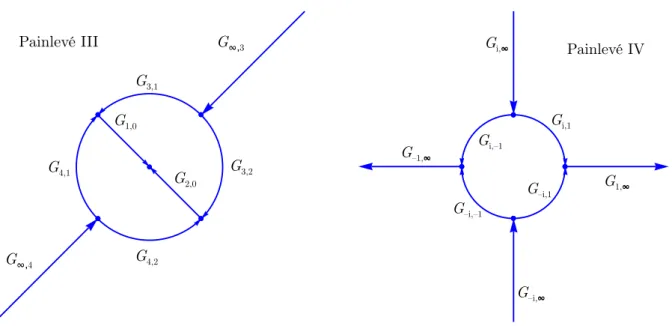
Table 1: Definitions for the Cauchy matrices.
Since C+− C− =I, we require that C+−C− = I, or in particular we define C−[Γ
i,Γi] as
C+[Γi,Γi]−I. In other words, we only need to construct C+.
We will sometimes simply refer toC+[Γi,Γj], which isC+[Γi,Γj] wheni=j andC[Γi,Γj]
otherwise. The goal of this section is to compute eachC+[Γi,Γj]: annΓj×nΓi matrix which
maps from values Ui at the points xi to something related to the Cauchy transform at the
points xj.
In the remainder of this section, we speak in terms of general domains Γ and Ω. We will assume attached to each domain is a vector of points xΓ and xΩ, with lengths nΓ and nΩ. Because these lengths are not necessarily the same, the matrix C[Γ,Ω] is rectangular and of dimensions nΩ×nΓ. Note that we combine these rectangular matrices to construct the square matrix C+.
We have several different situations to consider. See Table 1 for a guide for which definition is used to constructC+[Γ,Ω].
Cauchy matrices for the unit interval
Our first concern is to construct C+[I,I], essentially the process of computing the limit of the Cauchy transform of a function defined onIback on to itself. Recall from Theorem 4.1 that C+Tk(x) = − 2 iπTk(x)arctanhT −1 ↓ (x) + 1 iπ b(k+1)/2c X j=1 Tk−2j+1(x) 2j−1 1 k−2j+ 1 = 0 2 otherwise .
The easiest term corresponds to the bounded term, which is a polynomial. Forn =n
I odd,
we can write it in terms of the following n×n almost Toeplitz matrix:
P = 1 2 . .. 2 0 1 0 13 0 15 · · · 0 n−12 0 1 0 13 0 15 · · · 0 n−12 . .. ... ... ... ... ... 0 1 0 13 0 15 ... 1 0 13 0 15 1 0 13 0 1 0 13 1 0 1 0 .
The version for n odd is the Toeplitz matrix with its first row and column removed:
P = 1 2 . .. 2 0 1 0 13 0 15 · · · 0 n−11 . .. ... ... ... ... ... 0 1 0 13 0 15 ... 1 0 13 0 15 1 0 13 0 1 0 13 1 0 1 0 .
Now for the unbounded term, we note that we can simply evaluate the closed form expression for the Cauchy transform at xI with its endpoints removed: ¯xI = xI
2:n−1. All that remains is the value at the endpoints. We use the finite part of the singularity data for
this. From the definition of singularity data and (4.4), we find that FPL+ΨI(z)F =FPL+T0, . . . ,FPL+T0 F =aL0 −rL0iπ, . . . , anL−1−rnL−1iπF =−[log 2 + iπ]r0L, . . . , rLn−1F +1 iπ µ0(−1),−µ0(−1)−µ1(−1), . . . ,(−1)n−1(µn−2(−1) +µn−1(−1)) F = 1 iπ " log 2 2 + iπ 2 # e>L + 1 iπe > LPFU. Likewise, FPR+ΨI(z)F = 1 iπ " −log 2 2 + iπ 2 # e>R + 1 iπe > RPFU. We thus obtain Definition 5.1 C+[I,I] = 1 iπ log 2 2 + iπ 2 −2diag (arctanhT↓−1(¯xI)) −log 22 +i2π + 1 iπF −1PF.
Remark: If instead of constructing a matrix, we were concerned with evaluating the limit of the Cauchy transform from the left or right (which together give the finite Hilbert transform), an important observation that was missed in [15] is that P is a Toeplitz matrix plus a vector that only depends on the first row. In other words, we can evaluate the finite Hilbert transform of a function defined at thenChebyshev pointsxI at the same points inO(nlogn)
time.
We now consider the Cauchy matrix C[I,Γ], for Γ not connected to I. If n = n
I is
the degree of the Chebyshev interpolation, we require ψ1−n(T+−1(xΓ)), . . . , ψn−1(T+−1(xΓ)). Since computing hypergeometric functions is slow, we want to avoid their computation as much as possible. Fortunately from the first definition of ψk, we have a simple recurrence
relationship:
ψk(z) = zψk−1(z)−
2
iπk for oddk
0 otherwise .
For k > 0, we can first compute ψ0(z) via the arctanh function, and can in turn compute
ψ1(z), ψ2(z), . . .. Fork <0, we cannot start with the arctanh function and use the recurrence relationship in reverse: each term is subtracting out the Taylor series of the arctanh function, hence round-off error occurs. Instead, we computeψ1−n(z) using the hypergeometric function
representation, followed by the recurrence relationship again in the forward direction. This leads to the following algorithm:
Algorithm 5.2 Recurrence relationship
Given z∈Cm and n, compute the m×n matrix Ψz
n as follows: ψ1−n =ψ1−n(z), ψk =zψk−1− 2 iπk for oddk 0 otherwise for k = 2−n, . . . ,−1, ψ0 =ψ0(z), ψk =zψk−1− 2 iπk for oddk 0 otherwise for k = 1, . . . , n−1, Ψzn =−1 2(2ψ0,ψ−1+ψ1, . . . ,ψ1−n+ψn−1).
We can now successfully construct the necessary matrix:
Definition 5.3 If Γ is not connected to I, then, forz =T+−1(xΓ) and n=n
I, define
C[I,Γ] =ΨznF.
Now suppose the curve Γ is connected to the unit interval at one of its endpoints, for example the left endpoint of Γ is either±1: MΓ(±1) = −1. We can determineΨzn, but now
with all points in xΓ not connected to I: T+−1xΓ2:nΓ = T+−1
xΓ2, . . . , xΓnΓ>
. Then we take the finite part of the remaining term, using the fact that the angle that Γ leaves ±1 is
−argMΓ0(±1). To compute this, we will need the values
µ0(±1),±[µ1(±1) +µ0(±1)], . . . ,(±)n−1[µ1(±1) +µ0(±1)]. These are evaluated by simply summing the series term by term:
Algorithm 5.4 Taylor series
Given n, compute µLn/R (again, relating L with −1 and R with +1) as follows:
µ0= 0, µk =µk−1+ ( (±1)k k for odd k 0 otherwise for k = 1, . . . , n−1 µLn/R = 1 iπ µ0,±[µ0+µ1], . . .(±1)n−1[µn−2+µn−1] .
Definition 5.5 If MΓ(±1) = −1, then, for θ = −argMΓ0(±1), z = T+−1xΓ2:n Γ , n = n I and rL/R = r0L/R, . . . , rLn−/R1 = ±1 2iπ, . . . , (±1)n−1 2iπ ! , define C[I,Γ] = µ L/R n + h i arg±eiθ−log 2irL/R Ψz n ! F.
If MΓ(±1) = 1, then, forθ =−arg (−MΓ0(±1)), z =T+−1
xΓ1:nΓ−1 and n=n I, define C[I,Γ] = Ψ z n µLn/R+ h i arg±eiθ−log 2irL/R ! F.
The construction in the case both endpoints are connected toIis also clear, though omitted.
Curves Γwhose conformal map leaves ∞ at ∞
We now consider the matricesC+[Γ,Ω] such thatMΓ(∞) =∞. This naturally precludes the case where Γ is unbounded. From Theorem 4.2, we know that the Cauchy matrix is essentially unchanged, except for alterations of the singularity data. Thus we obtain the following constructions:
Definition 5.6 If MΓ(∞) =∞, then, for zL=MΓ−1(−1) andzR =MΓ−1(+1), define
C+[Γ,Γ] = C+[I,I] + 1 2iπ −log|MΓ0(zL)| log|MΓ0(zR)| .
Definition 5.7 If MΓ(∞) =∞ and Γ and Ω are disconnected, then define
C[Γ,Ω] =C[I, MΓ(Ω)],
where MΓ(Ω) is the domain resulting from conformally mapping Ω using MΓ.
Definition 5.8 Suppose MΓ(∞) = ∞, and let zL = MΓ−1(−1) and zR = MΓ−1(+1). If
zL =MΩ−1(−1), then define C[Γ,Ω] =C[I, MΓ(Ω)]− log|MΓ0(zL)| 2iπ 1 ,
where the last matrix is thenΩ×nΓ matrix with a one in the (1,1) entry and zeros elsewhere (similar notation is used below). IfzL=MΩ−1(+1), then define
C[Γ,Ω] =C[I, M(Ω)]− log|M 0 Γ(zL)| 2iπ 1 . If zR =MΩ−1(−1), then define C[Γ,Ω] =C[I, MΓ(Ω)] + log|MΓ0(zR)| 2iπ 1 . If zR =MΩ−1(+1), then define C[Γ,Ω] =C[I, MΓ(Ω)] + log|MΓ0(zR)| 2iπ 1 . Bounded curves
In this section, we assume that MΓ(∞) 6=∞, but where Γ is bounded. From (4.1), we know we must subtract out the behaviour of the Cauchy transform of where ∞ is mapped to under MΓ, and alter the finite part at the endpoints.
Definition 5.9 For z =T+−1(MΓ(∞)) and n=nΓ, define
C+[Γ,Γ] ={Definition 5.6} −1n×ndiag (Ψzn)F,
where 1k×l is the k×l matrix of all ones, and in this case Ψzn is a simply a row vector.
Definition 5.10 If Γ and Ω are disconnected, then, for z = T+−1(MΓ(∞)) and n = nΓ, define
C[Γ,Ω] =C[I, MΓ(Ω)]−1nΩ×ndiag (Ψ
z n)F.
Definition 5.11 If Γ and Ω are connected,then, for z =T+−1(MΓ(∞)) and n=nΓ, define
C[Γ,Ω] ={Definition 5.8} −1nΩ×ndiag (Ψ
z n)F.
Unbounded curves
We now consider the case where Γ is unbounded. In this case M(∞) is ±1, hence Algorithm 5.2 cannot be used, since the arctanh function blows up. But we know the basis vanishes at∞, thus we simply take the finite part.
Definition 5.12 IfMΓ(∞) =−1, then, for zR =MΓ−1(+1), n =nΓ and m =nI =n+ 1, define C+[Γ,Γ] = C+[I,I]2:m,2:m−1n×mdiag (µLm)FΓ+ log|MΓ0(zR)| 2iπ 1 .
If MΓ(∞) = +1, then, for zL =MΓ−1(−1), n=nΓ and m=nI =n+ 1, define
C+[Γ,Γ] =C+[I,I]1:n,1:n−1n×mdiag (µRm)FΓ− log|MΓ0(zL)| 2iπ 1 .
Definition 5.13 Suppose Γ and Ω are disconnected and let n =nΓ and m =nI = n+ 1. If MΓ(∞) =−1, then define C[Γ,Ω] =C[I, MΓ(Ω)]1:nΩ,2:m−1nΩ×mdiag (µ L m)FΓ. If MΓ(∞) = +1, then define C[Γ,Ω] =C[I, MΓ(Ω)]1:nΩ,1:n−1nΩ×mdiag (µ R m)FΓ.
Definition 5.14 Suppose Γ and Ω are disconnected and let n =nΓ and m =nI = n+ 1. If MΓ(∞) =−1, then define C[Γ,Ω] ={Definition 5.8}1:n Ω,2:m−1nΩ×mdiag (µ L m)FΓ. If MΓ(∞) = +1, then define C[Γ,Ω] ={Definition 5.8}1:n Ω,1:n−1nΩ×mdiag (µ R m)FΓ.
6. Properties of the approximate solution
We have described how we construct the matricesC±, thus we have everything necessary to construct the collocation system (2.3). Assuming it is nonsingular — which is satisfied, at least, for G sufficiently close to the identity matrix — we can solve this system to ob-tain U using a dense linear algebra package (in our case, we use Mathematica’s built-in LinearSolve, which is based onLAPACK). We thus obtain
˜ Φ(z) = I+CΦ(z)FU =I+ ` X k=1 CΦΓk(z)FΓkU k,
We must justify why ˜Φ can be considered an approximation to Φ. One posible issue is that ˜Φ is, as far as we know, unbounded. Another issue is that the values we assign forC±at the junction points of Γ are, a priori, unrelated to the value of the Cauchy transform of our basis, which blows up. The key to justifying the approximation is the following condition, which, when satisfied, will resolve both issues:
Definition 6.1 Givenξ ∈C, let {Ω1, . . . ,ΩL}be the subset of{Γ1, . . . ,Γ`}whose elements
contain ξ as an endpoint. Define pi = MΩi(ξ) = ±1, which determines if it is the left or
right endpoint, andUi =e>piUΩi, which is the value of the computed jump curve atξ (using
the convention that e−1=eni). The zero sum condition at ξ is satisfied if L
X
i=1
piUi = 0.
The zero sum condition is satisfied if the zero sum condition at every endpoint of Γ1, . . . ,Γ`
is satisfied.
Lemma 6.2 Suppose that the zero sum condition is satisfied. Then Φ(˜ z) =I +CΨ(z)FU is bounded and C±U = lim z→x1 for z onΓ1I+C ±Ψ(z)FU .. . lim z→x` for z onΓ`I+C ±Ψ(z)FU ,
i.e. applying C± is equivalent to computing the limit of the Cauchy transform of our ap-proximation at the points x.
Proof:
The only possible blow-up of the Cauchy transform is at an endpoint ξ of the curves which make up Γ. We will use the notation of Definition 6.1, and letθi =−arg
h
−piMΩ0i(ξ) i
be the angle at which Ωi leaves ξ. We have
˜ Φ(z) =I+CΨ(z)FU =I+ ` X k=1 CΨk(z)FkUk.
Asz approaches ξ, we note that the Cauchy transform of any curve not connected toξmust be bounded at ξ, hence lim →0 ˜ Φ(ξ+) = D+ lim →0 L X i=1 CΨΩi(ξ+)FΩiU Ωi.
Now each of these blows up atξ, however, we know precisely the singularity data. Thus, for constants D(i), depending only, possibly, on arg, we have
CΨΩi(ξ+)FΩiU Ωi ∼D (1) + logpie−iθi rpi0 , . . . , rnpiΩ i−1 > FΩiU Ωi
=D(2)+hlog||+ i argpie−iθi
ipiUi 2πi (due to (4.4)) =D(3)arg+ log||piUi 2πi Thus we have ˜ Φ(ξ+)∼Darg(4)+ log|| 2πi L X i=1 piUi=D(4)arg,
which proves that it is bounded at ξ.
The value we assigned to the Cauchy matricesC±[Γi,Γj] at points which are not junction
points was, by definition, the Cauchy transform. The value we chose at each endpoint was chosen to be the limit of the Cauchy transform, ignoring the unbounded term which grew like log|z|. We have shown that each of these unbounded terms is cancelled, therefore, the second part of the lemma follows.
Q.E.D.
What is clear from this lemma is that it is important that the zero sum condition is sat-isfied in order for our approximation to Φ to be analytic, hence a reasonable approximation to the actual Φ. Now we have not (as of yet) imposed the zero sum condition; however, the following condition on the jump curve G (hence completely independent of the discretiza-tion), which should almost always be satisfies, will automatically imply that the zero sum condition is satisfied:
Definition 6.3 Let{Ω1, . . . ,ΩL}denote the subset of{Γ1, . . . ,Γ`} whose elements contain
ξ as an endpoint, θi the angle at which Ωk leaves ξ, pi = +1 if ξ is the left endpoint and
−1 if ξ is the right endpoint of Ωi and let Gi be the limit of G(z) as z approaches ξ along
Ωi. We assume that{Ω1, . . . ,ΩL}is sorted so thatθi is strictly increasing. The nonsingular
junction condition at ξ is satisfied if
(θL−θ1)I+
L X
k=2
(θk−1−θk)Gpkk· · ·GpLL
is nonsingular. The nonsingular junction condition is satisfied if the nonsingular junction condition at every endpoint of Γ1, . . . ,Γ` is satisfied.
Theorem 6.4 Suppose that the RH problem is well-posed, the collocation system has a solution and the nonsingular junction condition is satisfied. Then the computed vector U satisfies the zero sum condition and Lemma 6.2 applies.
Proof:
This theorem is a generalization of Theorem 4.2 from [14]. We reuse the notation of Lemma 6.2. For simplicity in notation, we assume every curve Ω1, . . . ,ΩL has ξ as a left
endpoint; the generalization for other cases is straightforward.
Note that (since θi < θj for i < j) the finite part of each UΩi along Ωj is
FPLθj/RUΩi =ai+ iriarg −ei(θj−θi)=ai+ iri θj−θi−π if i < j θj−θi+π if i > j ,
where ai and ri are some constants. We thus define
Θ± = ∓π θ1−θ2+π · · · θ1−θL−1+π θ1−θL+π θ2−θ1−π ∓π θ2−θ3+π · · · θ2−θL+π .. . . .. . .. . .. ... θL−1−θ1−π · · · θL−1−θL−2−π ∓π θL−1−θL+π θL−θ1−π θL−θ2−π · · · θL−θL−1−π ∓π .
LetUi =e>LUΩi denote the value of UΩi atξ, and we note thatri =− Ui
2πi. Therefore, if we can show that
S =
L X
i=1
ri
is zero, the zero sum condition at ξ follows.
Let oi denote the index of the collocation point in x corresponding to ξ along Ωi. For
the vectorr = (r1, . . . , rL)>, We can write theLcomputed values corresponding to the limit
of the Cauchy transform along each Ωi as
Φ±= Φ±1 .. . Φ±L = I .. . I + e>o1 .. . e>oL C±U = D .. . D + Θ ±r.
The constant D consists of contributions which are independent of the angle at which ξ is approached: the contributions ofU from curves not in{Ω1, . . . ,ΩL}, as well as the constants
ai. Since
e>i Θ+=e>i+1Θ−+θi+1−θi, (here we identifyL+ 1 with 1)
we have
Furthermore, the collocation system implies that Φ+i = Φ−i Gi. Thus we get: Φ+L = Φ−LGL = Φ+L−1GL+S[(θL−1−θL)GL] (6.1) = Φ−L−1GL−1GL +S[(θL−1−θL)GL] = Φ+L−2GL−1GL +S[(θL−2−θL−1)GL−1GL+ (θL−1−θL)GL] .. . = Φ+LG1· · ·GL+S L X i=2 (θi−1−θi)Gi· · ·GL.
The well-posedness of the RH problem requires that:
G1· · ·GL =I. Hence we obtain 0 =S (θL−θ1)I+ L X i=2 (θi−1−θi)Gi· · ·GL .
By assumption the term in brackets is nonsingular, which implies that S = 0 and the zero sum condition at ξ follows. Applying this to each endpoint ξ proves the theorem.
Q.E.D.
This theorem could potentially have consequences for the analytical solution: what it states is that, generically, we need not impose that the solution to the RH problem is bounded at the junction points, since it follows from the nonsingular junction condition.
The nonsingular junction condition is independent of the well-posedness of the RH prob-lem, so if we are unfortunate we can find ourselves in a situation where it is not satisfied. Indeed, in [14], Stokes’ multipliers to the Painlev´e II transcendent were chosen particularly so that this condition was not satisfied. What was noted in this case was that the collocation system itself became singular: it had multiple solutions. Therefore, the zero sum condition could be appended to the linear system, to enforce that the solution chosen satisfied the zero sum condition. The following corollary states that this phenomena is true in general:
Corollary 6.5 Suppose the nonsingular junction condition is not satisfied at a junction
ξ. Using the notation of the previous theorem, consider the collocation system with the condition
replaced with
L X
i=1
piUi = 0.
If the resulting system is nonsingular, thenΦ+L = Φ−LGL is still satisfied. Since the computed
solutionU satisfies the zero sum condition, Lemma 6.2 applies.
Proof:
Consider (6.1). We cannot begin with Φ+L; we do not know a priori that Φ+L = Φ−LGL. However, the remaining equalities still hold, and we have
Φ−LGL = Φ+L +S L X k=1 (θk−1−θk)Gk· · ·GL = Φ+L, since S =−21πiP Ui= 0. Q.E.D. 7. Examples
We apply this numerical approach to two examples, taken directly from [8], though we make the construction of the RH problems explicit. We have also fixed several typos from [8]. In a way this helps to demonstrate another important aspect of having a numerical approach: it helps confirm (and in this case, correct) analytic formulæ.
Painlev´e III
Our first example is the Painlev´e III RH problem, for solving the Painlev´e III differential equation: d2u dx2 = 1 u du dx !2 − 1 x du dx + 4 x Θ0u2+ 1−Θ∞ + 4u3− 4 u.
Related to u is the variable y, which satisfies dy dx = Θ∞ x y+ 2y u .
What follows is the construction of a RH problem Φ+(x;z) = Φ−(x;z)G(x;z) so thaty(and thence u) is determined from Φ. We restrict our attention to the case where x is positive and real for simplicity: the curve Γ of the RH problem depends on the phase of x.
Rather than specifying initial conditions, we specify Stokes’ multipliers s(0)1 , s(0)2 , s(1∞)
and s(2∞), which satisfy the equation 2 cosπΘ0+s (0) 1 s (0) 2 e− iπΘ0 = 2 cosπΘ ∞+s(1∞)s (∞) 2 e iπΘ∞.
(In [8], two conflicting versions of this equation are stated. The equation presented here is
indeed the correct one.) This equation ensures that the RH problem that is constructed is well-posed.
Often in physical applications it is the Stokes’ multipliers which are known. What follows can be considered as a numerical map from Stokes’ multipliers to initial conditions. Moreover, this map could potentially be inverted to map initial conditions to Stokes’ multipliers. Since the Stokes’ multipliers determine the asymptotic behaviour of the solution u, this could be used to connect asymptotic behaviour to initial conditions.
In this example, we choose (arbitrarily) Θ0= 3.43, Θ∞ = 1.123 s(0)1 = 1, s(0)2 = 2, s(1∞) = 3, s(2∞) = (−1).8772 3 (−1).57+ cos.123π−sin.07π =−0.5477638340114221...−0.4795328603546345...i.
To construct the jump curves, we need a matrix E that satisfies
1 +s(1∞)s(2∞) s(1∞) s(2∞) 1 eiπΘ∞ e−iπΘ∞ =E−1 1 +s(0)1 s(0)2 s(0)1 s(0)2 1 e−iπΘ0 eiπΘ0 E.
ThusE can be viewed as a generalized eigenvector matrix. One choice (found symbolically) is E = 0.966469141021...+ 1.068382000028...i 0.778294876111...−0.163709626483...i 1 1 .
We will also need to use a power function with a nonstandard branch cut. We define the power function with branch cut along angle t as
zy,t =ei(−π−t)zye−i(−π−t)y.
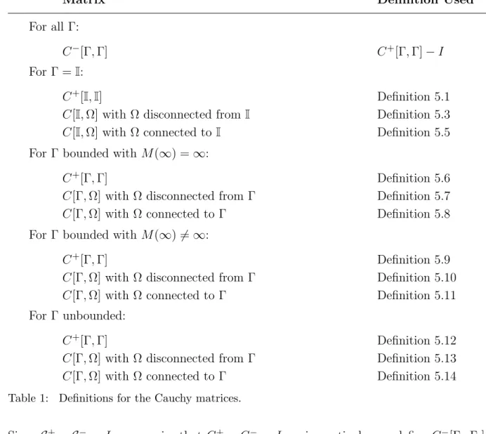
We can now construct the RH problem. The left graph of Figure 2 depicts the jump curve Γ, along which we define the jump curves Gi,j: for the function θ(x;z) = i2x
G3,2 G4,2 G2,0 G1,0 G∞,3 G∞,4 G4,1 G3,1 Painlevé III G1,∞ Gi,∞ G–i,∞ G–1,∞ Gi,–1 Gi,1 G–i,1 G–i,–1 Painlevé IV
Figure 2: The jump curves for the Painlev´e III (with junction points at0,e−5iπ/4,e−iπ/4,eiπ/4, e5iπ/4 and ∞) and Painlev´e IV (with junction points at−1,−i,1,iand ∞) RH problems.
we have G3,2= e θzΘ0/2 e−θz−Θ0/2 ! E zΘ∞/2e−θ z−Θ∞/2eθ ! , G∞,3= 1 −s (∞) 1 e2θz−Θ∞ 0 1 ! , G4,0 = 1 −s (0) 1 e2θzΘ0 0 1 ! , G1,4= e θzΘ0/2,−π/2 −s(0) 1 eθzΘ0/2,−π/2 e−θz−Θ0/2,−π/2 ! E zΘ∞/2,−π/2e−θ s (∞) 1 z−Θ∞/2,−π/2eθ z−Θ∞/2,−π/2eθ ! , G1,2= e θz−Θ∞/2 e−θzΘ∞/2 ! E−1 z−Θ0/2,0eiπΘ0−θ −s(0)2 z−Θ0/2,0e−iπΘ0−θ zΘ0/2,0eθ−iπΘ0 ! , G3,4= e θz−Θ∞/2 −s(∞) 1 eθz−Θ∞/2 e−θzΘ∞/2 ! E−1 z−Θ0/2e−θ zΘ0/2eθ ! , G2,0= 1 −s(0)2 e−2θz−Θ0,0 1 ! and G∞,1 = 1 −s(2∞)e−2θzΘ∞,−π/2 1 ! .
Along each curve, we need to decide at how many points to sample. We choose this adaptively: we take sufficiently many points so that the omitted terms of the Chebyshev expansion are each less than a given tolerance.
We can now apply our numerical approach to determine an approximation ˜Φ. However, we are really interested in the solution u to the Painlev´e III ODE. We have the following
definition:
y(x) =−ix lim
z→∞zΦ12(x;z) = −ixzlim→∞z[CU(x;z)]12,
where 12 denotes the (1,2) entry of the matrix. (In [8], this was mistakenly given as a definition for u(x).) But the limit of the Cauchy transform is simply an integral of the function: lim z→∞zCU(z) = 1 2πi Z Γ z t−zU(t) dt =− 1 2πi Z ΓU(t) dt. Moreover, we can evaluate this integral by transforming to the unit interval
Z ΓU(t) dt= X i Z Γi Ui(t) dt = X i Z 1 −1 Ui(Mi−1(p)) M0(Mi−1(p))dp.
Each of these integrals can be evaluated with Clenshaw–Curtis quadrature [3]. This quadra-ture routine computes an integral over I inO(nlogn) time using the value of the integrand at the nodesxI. In our case, the values are simplyUi, with a zero appended in the case that
Γi is unbounded, multiplied entrywise by M0
Mi−1xI−1. We define this approximation as QΓiUi. We thus obtain the approximation
Z ΓU(t) dt≈ QU = X QΓiUi, and hence y(x)≈ x 2πQU.
Now to findu, we will use the definition
u= 2xy
xyx−Θ∞y .
However, to obtain u, we need to compute yx at x. Fortunately, derivatives commute with
the limit, hence
yx(x) = −i limz→∞zΦ12(x;z)−ixzlim→∞zΦx,12(x;z).
We already have computed Φ12, but we now also need the derivative of Φ with respect to x. This is straightforward by simply differentiating the RH problem:
Φ+x −Φ−xG= Φ−Gx and Φx(∞) = 0.
Replacing Φx by CUx, we see that this equation is of exactly the same form as (2.1), with
only a different right hand side. Therefore, having constructedU, we can determine a vector Ux by reusing the matrix of (2.3) (hence all the computed Cauchy matrices) to solve
h C+−rdiag (G)C−iUx = rdiag (Gx(x)) I .. . I +C −U .
3.5 4.0 4.5 5.0 -2.5 -2.0 -1.5 -1.0 -0.5 0.5 3.5 4.0 4.5 5.0 10-8 10-7 10-6 10-5 10-4
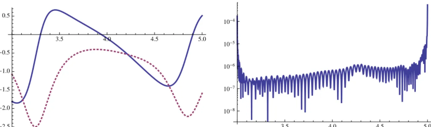
Figure 3: The real (solid line) and imaginary (dotted line) parts of a solution to Painlev´e III on the left, with its relative error in residual on the right.
Thus we obtain
u(x)≈ 2x[QU]12
x[QUx]12+ (1−Θ∞) [QU]12 .
In Figure 3, we plot the computed solution, and demonstrate that it does satisfy the Painlev´e III ODE by finding the error in residual, computed by evaluating the approximation at 85 mapped Chebyshev points between 3 and 5. In this case seven digits of accuracy are about how many can be expected: the last Chebyshev coefficient is on the order of 10−10 and two derivatives should multiply the error by about 852 ≈104.
Perhaps a more useful calculation would be the Sine–Gordon reduction to Painlev´e III. This has a significantly simpler RH formulation, consisting of four rays emanating from the origin. We instead chose the more general Painlev´e III RH problem, to demonstrate the flexibility of the framework.
Painlev´e IV
We now consider the Painlev´e IV RH problem, for computing the solutions to the Painlev´e IV ODE: d2u dx2 = 1 2u du dx !2 + 3 2u 3+ 4xu2+ 2 + 2x2−4Θ∞ u− 8Θ 2 u ,
where Θ∞ and Θ are constants. Solutions are specified by the four Stokes’ multipliers s1, s2, s3 and s4, satisfying the relationship
(1 +s2s3)e2iπΘ∞ + [s1s4+ (1 +s3s4)(1 +s1s2)] e−2iπΘ∞ = 2 cos 2πΘ. Again, we choose these constants arbitrarily:
Θ = 3.43, Θ∞= 1.123 s1 = 1, s2= 2, s3 =
1 3,
100 200 300 400 500 N 10-11
10-8 10-5 0.01
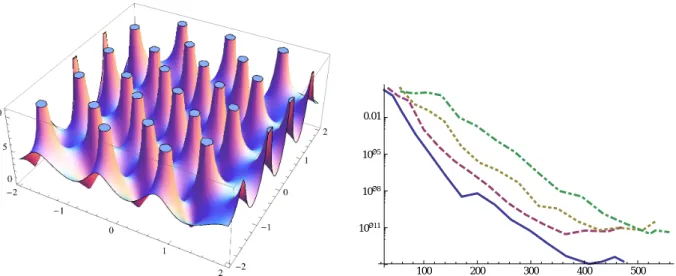
Figure 4: On the left, a plot of the absolute value of a solution to Painlev´e IV in the complex plane. On the right, the relative error of the approximation forx= 0(solid), 1 (dashed), 2 (dotted) and 3 (dash and dotted).
We also need a matrix E, but in this case it is simply an eigenvector matrix (where we happen to know the eigenvalues)
1 s1 1 1 s2 1 1 s3 1 1 s4 1 e 2iπΘ∞ e2iπΘ∞ =E−1 e−2iπΘ e2iπΘ E.
The right graph of Figure 2 depicts the jump curve Γ, along which we define the jump curves
Gi,j for θ(x;z) = z 2 2 +xz: G−i,−1 = eθzΘ,0 e−θz−Θ,0 E (1 +s2s3)zΘ∞,0e−θ s2z−Θ∞,0eθ (s1+s3+s1s2s3)zΘ∞,0e−θ (1 +s1s2)z−Θ∞,0eθ ! , G−i,1 = eθz−Θ∞ e−θzΘ∞ E−1 z−Θe−θ zΘeθ , Gi,1 = eθzΘ e−θz−Θ E zΘ∞e−θ s1zΘ∞e−θ z−Θ∞eθ , Gi,−1 = (1 +s1s2)e θz−Θ∞,0 −s 2eθz−Θ∞,0 −s1e−θz0Θ∞ e−θzΘ∞,0 ! E−1 z−Θ,0e−θ zΘ,0eθ , G−1,∞ = 1 s3e−2θz2Θ∞,0 1 , G∞,−i= 1 −s4e2θz−2Θ∞,0 1 , G1,∞ = 1 s1e−2θz2Θ∞ 1 and G∞,i = 1 −s2e2θz−2Θ∞ 1 .
collocation points on each curve adaptively. The relation between Φ andu is u(x) = −2x− lim z→∞∂xlog Φ12(x;z) = −2x−zlim→∞ Φx,12(x;z) Φ12(x;z) . Thus we define u(x)≈ −2x− [QUx]12 [QU]12.
In the left graph of Figure 4, we plot the absolute value of a solution to Painlev´e IV in the complex plane. Note the presence of poles. This is one aspect where our method outperforms a standard ODE solver; integrating past poles is not an issue, since xis merely a parameter. At the pole, the RH problem does not have a solution. This manifests itself in our numerical approach by a badly condition collocation system.
In the right graph of Figure 4, we compare the convergence of the approximation as
N (the total number of collocation points) increases, where the distribution of number of points on each curve is chosen adaptively. We compare these approximations with the approximation found with a much larger value of N. Spectral convergence and stability of the method is clear, as is the slower convergence rate as xbecomes large.
8. Conclusions and future work
We have constructed a framework for computing RH problems, and demonstrated its effectiveness by applying it to the computation of Painlev´e transcendents. The world of RH problems is large, and this opens up a new numerical technique applicable to fields from integrable systems to orthogonal polynomials and random matrix theory. It is our belief that many problems exist in these fields which, while at first seemingly intractable from a numerical perspective, can now be efficiently and reliably computed.
We have provided an implementation of this framework inMathematicainRHPackage
[13], including the implementation of the two examples from this paper. The only piece that cannot be translated to an alternate programming language in a straightforward manner is the computation of hypergeometric functions used as the seed to Algorithm 5.2, as built-in routines for hypergeometric functions in, say, Matlabare not reliable [16]. However, there are many methods for computing hypergeometric functions [12], and it is possible that one of these is accurate and reliable in the regime we are interested in.
What makes RH problems so powerful in an analytic context is nonlinear steepest de-scent; the problem can be deformed so that oscillations (as seen in our two examples) become exponential decay. While our numerical approach breaks down in the two examples asx be-comes large, using the deformed contour will allow high accuracy in the asymptotic regime. However, the resulting paths of steepest descent are not trivially deformable to the unit interval, hence the framework constructed cannot be directly applied. However, errors in the
path of steepest descent do not result in errors in the approximation, and thus the path can be replaced by a piecewise affine interpolant.
An example application of this is the Hastings–McLeod solution [9] to Painlev´e II, which has applications in random matrix theory via the Tracy–Widom distribution [17]. Pertur-bations of the initial conditions result in either high oscillations or poles, neither of which is present in the true solution. In [14], we demonstrated that it can be computed near the ori-gin using the current framework; or, alternatively (and more efficiently), using the Fredholm determinant representation [2]. Both approaches break down as x becomes large; however, using the deformed contour will result in a reliable numerical method for allx. This will be the topic of a future paper.
This framework has been based on the Chebyshev basis. Another possible basis are the Legendre polynomials, whose Cauchy transforms decay to high asymptotic order due to orthogonality: CPk(z) = 1 2πi Z 1 −1 Pk(x) x−z dx= 1 2πizk Z 1 −1 Pk(x)xk x−z dx=O z−k−1.
This could lead to sparser matrices, and, potentially, a faster solution of the collocation system. Moreover, an explicit formula is known:
CPk(z) = − 2k+1(k!)2 2πi(2k+ 1)!(z−1)k+1 2F1 k+ 1, k+ 1 2k+ 2 ; 2 1−z ! . [7]
However, we have used the Chebyshev basis in this paper due to the availability of a fast and accurate transform between a set of nodes which include the endpoints and the series’ coefficients.
One last issue that must be resolved is a proof of convergence. Assuming the RH problem has a solution, it is our feeling that convergence of the numerical approximation should follow, since C+U −hC−Ui
G is a bounded linear operator from the space of H¨older-continuous functions U defined on Γ which satisfy (the infinite dimensional version of) the zero sum condition to the space of H¨older-continuous functions U defined on Γ. Indeed, all numerical experiments have shown clear and stable convergence, depending only on the condition number of the collocation system. However, since the domain space and range space of this operator differ, the standard convergence proofs for collocation methods do not apply. Acknowledgments: I thank Alex Barnett, discussions with whom lead me to Algorithm 5.2, Andrew Dienstfrey, who pointed me to his thesis, and Andre Weideman, who recommended replacing Lerch transcendents with hypergeometric functions.
References
[1] Ablowitz, M.J. and Segur, H., Solitons and the Inverse Scattering Transform, SIAM, 2006.
[2] Bornemann, F., On the numerical evaluation of Fredholm determinants, Maths Comp
79 (2010), 871–915.
[3] Clenshaw, C. W. and Curtis, A. R., A method for numerical integration on an automatic computer, Numer. Math. 2 (1960), 197–205.
[4] Deift, P., Orthogonal Polynomials and Random Matrices: a Riemann-Hilbert Approach, AMS, 2000.
[5] Deift, P. and Zhou, X., A steepest descent method for oscillatory Riemann-Hilbert problems, Bulletin AMS 26 (1992), 119–124.
[6] Dienstfrey, A., The Numerical Solution of a Riemann-Hilbert Problem Related to Random Matrices and the Painlev´e V ODE, Ph.D. Thesis, Courant Institute of Mathematical Sciences, 1998.
[7] Elliott, D., Uniform asymptotic expansions of the Jacobi polynomials and an associated function, Maths Comp. 25 (1971), 309–315.
[8] Fokas, A.S., Its, A.R., Kapaev, A.A. and Novokshenov,V.Y., Painlev´e transcendents: the Riemann-Hilbert approach, AMS, 2006.
[9] Hastings, SP and McLeod, JB, A boundary value problem associated with the second Painlev´e transcendent and the Korteweg-de Vries equation,Archive for Rational Mechanics and Analysis 73 (1980), 31–51.
[10] Muskhelishvili, N.I., Singular Integral Equations, Groningen: Noordhoff (based on the second Russian edition published in 1946), 1953.
[11] Nasser, M.M.S., Numerical solution of the Riemann-Hilbert problem, Punjab University Journal of Mathematics 40 (2008), 9–29.
[12] Olver, F. W. J., Lozier, D. W., Boisvert, R. F. and Clark, C. W., NIST Handbook of Mathematical Functions, Cambridge University Press, 2010.
[13] Olver, S., RHPackage, http://www.comlab.ox.ac.uk/people/ Sheehan.Olver/projects/RHPackage.html
[14] Olver, S., Numerical solution of Riemann–Hilbert problems: Painlev´e II, preprint, NA-09/09, Maths Institute, Oxford University.
[16] Pearson, J., Computation of Hypergeometric Functions, MSc. Thesis, University of
Oxford, 2009.
[17] Tracy, C.A. and Widom, H., Level-spacing distributions and the Airy kernel, Comm. Math. Phys.159 (1994), 151–174.
[18] Wegert, E., An iterative method for solving nonlinear Riemann-Hilbert problems, J. Comp. Appl. Maths 29 (1990), 327.
[19] Wegmann, R., Discrete Riemann-Hilbert problems, interpolation of simply closed curves, and numerical conformal mapping, J. Comp. Appl. Maths23 (1988), 323–352.
[20] Wegmann, R., An iterative method for the conformal mapping of doubly connected regions,J. Comp. Appl. Maths 14 (1986), 79–98.