Kernel Coherence Encoders

Worcester Polytechnic Institute

Digital WPI

Masters Theses (All Theses, All Years) Electronic Theses and Dissertations

2018-04-23

Kernel Coherence Encoders

Fangzheng Sun

Worcester Polytechnic Institute

Follow this and additional works at:https://digitalcommons.wpi.edu/etd-theses

This thesis is brought to you for free and open access byDigital WPI. It has been accepted for inclusion in Masters Theses (All Theses, All Years) by an authorized administrator of Digital WPI. For more information, please [email protected].

Repository Citation

Sun, Fangzheng, "Kernel Coherence Encoders" (2018).Masters Theses (All Theses, All Years). 252.

WORCESTER POLYTECHNIC INSTITUTE

Kernel Coherence Encoders

by Fangzheng Sun

A thesis

Submitted to the Faculty of the

WORCESTER POLYTECHNIC INSTITUTE in partial fulfillment of the requirements for the

Degree of Master of Science in

Data Science

April 2018

APPROVED:

Professor Randy C. Paffenroth, Adviser:

Contents

2.1.1 Weight Matrix and Bias Vector . . . 11

2.1.2 Non-linear Activation Function . . . 11

2.2 Autoencoders . . . 12

2.3 Canonical Correlation Analysis . . . 13

2.4 Kernel Methods . . . 15

2.4.1 Positive Definite Kernel . . . 16

2.4.2 Schoenberg’s Theorem . . . 16

2.5 KCCA . . . 17

2.6 Principal Component Analysis . . . 18

3 Model Design 20 3.1 Non-Coherence Encoder (NCE) . . . 21

3.1.1 Encoder Phase . . . 22

3.1.2 Decoder Phase . . . 22

3.2 Coherence Encoder (CE) . . . 24

3.2.1 Encoder Phase . . . 24

3.2.2 Decoder Phase . . . 25

3.3.1 Encoder Phase . . . 26 3.3.2 Decoder Phase . . . 28 4 Numerical Results 29 4.1 Data Sets . . . 29 4.2 Implementation Detail . . . 31 4.2.1 TensorFlow . . . 31

4.2.2 Gradient Descent Optimization . . . 31

4.2.3 Training Parameters . . . 32

4.3 Evaluation Metrics . . . 32

4.3.1 L2_{-Norm . . . . 33}

4.3.2 Pearson Correlation Score . . . 33

4.3.3 Cross-correlation . . . 34

4.3.4 Bhattacharyya Distance . . . 35

4.3.5 FFT Rank . . . 35

4.4 Reconstruction Images . . . 36

4.4.1 Simple ANNs Reconstruction . . . 36

4.4.2 NCE, CE and KCE Reconstruction . . . 38

4.5 Quantitative Comparison . . . 40

5 Conclusion 42 5.1 Contribution . . . 42

5.2 Future Work . . . 42

WORCESTER POLYTECHNIC INSTITUTE

Abstract

Data Science

Master of Science

by Fangzheng Sun

In this thesis, we introduce a novel model based on the idea of autoencoders. Different from a classic autoencoder which reconstructs its own inputs through a neural network, our model is closer to Kernel Canonical Correlation Analysis (KCCA) and reconstructs input data from another data set, where these two data sets should have some, perhaps non-linear, dependence. Our model extends traditional KCCA in a way that the non-linearity of the data is learned through optimizing a kernel function by a neural network. In one of the novelties of this thesis, we do not optimize our kernel based upon some prediction error metric, as is classical in autoencoders. Rather, we optimize our kernel to maximize the “coherence” of the underlying low-dimensional hidden layers. This idea makes our method faithful to the classic interpretation of linear Canonical Correlation Analysis (CCA). As far we are aware, our method, which we call a Kernel Coherence Encoder (KCE), is the only extent approach that uses the flexibility of a neural network, while maintaining the theoretical properties of classic KCCA. In another one of the novelties of our approach, we leverage a modified version of classic coherence which is far more stable in the presence of high-dimensional data to address computational and robustness issues in the implementation of a coherence based deep learning KCCA.

Chapter 1

Introduction

In the recent years, the concept of deep learning [23] is becoming a hot topic for divergent industries as well as multiple fields of study [9,14,18,40]. Deep learning is a subfield of machine learning and there are many sub-categories of deep learning itself. Herein, we focus on artificial neural networks (ANN) [24, 25] and autoencoders [2–4] that allow us to discover non-linear low-dimensional manifolds. Such methods are frequently used for unsupervised learning and for producing low-dimensional representations of data. Typically, an autoencoder consists two parts, an encoding phase (encoder) E(·) and a decoding phase (decoder) D(·). The encoder E(·) takes the input data and maps it to a low-dimensional representation. The decoder D(·) then takes this low-dimensional representation and attempts to reconstruct the original high-dimensional data.

Note, such an autoencoder is closely related to Principal Component Analysis (PCA) [6, 7, 17, 27]. In fact, an autoencoder is identical to PCA when each layer is assumed to be linear and the reconstruction cost function is Euclidean distance. In particular, many people are attracted by the nonlinear aspect of autoencoders, which makes it more powerful than PCA, and effective in solving real-life problems.

We create three novel models to leverage the full power of the autoencoders. Our first model, a Non-Coherence Encoder (NCE), is built upon both linear and non-linear autoencoders. Then we move on to CCA [5,13] and KCCA [1], merging their strengths with the autoencoder approach in another two proposed models, namely the Coherence Encoder (CE) and the Kernel Coherence Encoder (KCE). When we test their performance using the MNIST [39] digit image data set, we find that with these novel generalizations of CCA, especially KCCA, the predictions of images tend to be closer to the true images.

1.1

Motivation

Let us begin the story of our research with some interesting questions one may have: at the age of 20, can you predict how you will look at the age of 40? Or, when you look at a 40-year-old person, can you imagine what he or she looks like at the age of 20? A human brain, based on visual observations, learns and finds a “mapping” between a 20-year-old face and a 40-year-old face. Consequently, people might be able to give reasonable answers to the above questions. We want our model to mimic this learning process while maintaining its own ability to extract the “dependencies” between data sets. Our purpose is to reconstruct two “potentially dependent datasets” from each other. A classic autoencoder focuses on one input data set. However, we are interested in working with two dependent data sets and therefore we introduce CCA and even further its kernel version KCCA to extract the dependencies between them.

The earliest idea, of which we are aware, of applying kernel methods to autoencoders comes from Yan Pei’s work Auto-encoder Using Kernel Methods [9]. In his model, the author replaces the encoder part of an autoencoder with Kernel PCA (KPCA) [27] and the decoder with kernel-based linear regression. It is a model that is designed to work similarly to an autoencoder, but remains faithful to the “kernel trick”. The “kernel trick”, which will be discussed in detail in the next Chapter, is a classic technique for non-linearly projecting features to a high-dimensional space, gaining the benefit of complex non-linear features, without incurring the cost of working directly in a high-dimensional space. Although it is reasonable, and perhaps even obvious, to try to connect the kernel trick and deep learning, it is notable that, as far as we are aware, the current methods such as [9], do not leverage the full power of autoencoders.

1.2

Contribution

NCE is our model that is least faithful to the kernel trick and is built on two independent autoencoders containing both linear and nonlinear layers. Each “autoencoder” maps one data set to the other. However, this model is not theoretically well founded and the experimental results with MNIST digit image data indicate its deficiency.

Our improvements to the NCE model are inspired by CCA through Empirical canonical corre-lation analysis in subspaces [5]. This paper provides detailed explanations of CCA, including the calculations for canonical variables of data pairs. In particular, we are inspired by the authors’ idea to maximize their coherence through CCA. CCA and PCA differ in that PCA

attempts to reconstruct a set of data from itself, while CCA has two data sets, and it tries to reconstruct one data set from the other. It is this added complexity of having two data sets that make our proposed model non-trivial to develop.

However, in most real-life problems, the correlations of the data sets are not necessarily linear, thus calculating their linear coherence may not be the best solution to extract their depen-dencies. We take a further step by analyzing CCA’s kernel version, KCCA. With the help of deep learning, we develop a kernel function with a set of hyperparameters and train the kernel function to maximize the coherence of two data sets in the high-dimensional space. Then we extract the canonical variables for data reconstruction.

In another two models, CE and KCE, we take advantage of CCA and KCCA respectively. While CE rests upon the combination of linear CCA and autoencoders, in KCE we extend the traditional CCA from linear to non-linear by kernel methods and increase the performance of CCA in a similar way by leveraging the non-linear capabilities of autoencoders.

At a high level, our KCE method proceeds in two phases that are similar to autoencoders, the

encoder phase and thedecoder phase. First, we train the “encoder” to take our input data and map it to a space called a Reproducing Kernel Hilbert Space (RKHS) [10] by a particular kernel function, where the coherence between the input data is maximized. Note, this kernel function is trained through the “encoder”. With this well-trained kernel function, represented by the encoder, we can maximize the coherence of two potentially dependent datasets by mapping them to a high-dimensional space where their correlations become linear and much easier to be explored. Second, we fix the “encoder”, and then train the “decoder” comprised of neural networks to reconstruct our original two data sets.

Notably, we solve two problems caused by high dimensionality of data. First, the training process for such methods is very slow. To fix this issue, we apply PCA to the original dataset to decrease the dimension to an acceptable level, where the principal components carry most of the information of original data (explain >90% variance). Second, CCA is very sensitive to high-dimensionality because the high-dimensional Grammian matrix [11] containing the inner products can easily become close to singular [12] in the new space. So, it becomes difficult to calculate its determinant, as is required by using a coherence metric. In our model, we slightly modify the formula provided by [5] to avoid this issue at a cost of losing some computational efficiency. The modifications will be detailed in Chapter 3.

networks and PCA reconstruction to map the principal components back to the original space of another data set.

Using the MNIST digit image data experiment, we test the performance of NCE, CE, and KCE separately and then compare their reconstruction results with each other. The reconstruction images demonstrate a great visible advantage of the latter two models over NCE. On the other hand, supported by multiple quantitative metrics, we claim that KCE generates better reconstruction images than CE does.

Chapter 2

Background

In this Chapter, we will introduce the necessary background that forms our ideas and algo-rithms. First, we will cover deep learning and autoencoders. Our model is based on these ideas and inspired by the exploration of them. In our model, a deep learning approach is used to train the kernel function and to build linear and non-linear mapping processes in the decoder phase, which is very close to a classic autoencoder. Then, we give a detailed explanation as well as theoretical support for our encoder phase, the most significant novelty for our model. In particular, our encoder is quite different from a classic autoencoder. We will start from classical linear CCA and extend to kernel methods (by defining the kernel trick) and then proceed to nonlinear KCCA. Here we provide definitions and fundamental theorems used in our model and their theoretical background. Meanwhile, we will introduce the concept of coherence, the metric used by our model to optimize the kernel function. As we mentioned, we apply PCA to the original data set to avoid the dimensionality issue and improve computational efficiency. Thus we also cover the dimension reduction algorithm PCA at the end of this chapter.

2.1

Deep Learning

Our introduction to deep learning closely follows the definitions provided by [23]. Deep learning is a class of machine learning techniques that exploit many layers of non-linear information processing for supervised algorithms, such as pattern analysis and classification. It is a sub-field within machine learning that is based on algorithms for learning multiple levels of representation in order to model complex relationships among data. An observation (e.g., an image) can be represented in many ways (e.g., a vector of pixels), but some representations make it easier to

learn tasks of interest from examples, and research in this area attempts to define what makes better representations and how to learn them [23]. In this Section, we will focus on a narrower, but now commercially important, subfield of Deep Learning called artificial neural networks (ANN).

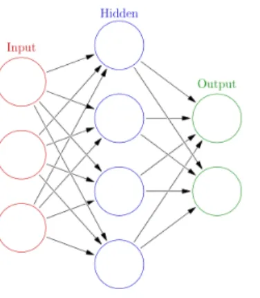
[24] gives us a standardized definition for ANN: For A standard ANN consists of many simple, connected processors called neurons, each producing a sequence of real-valued activations. In-put neurons get activated through sensors perceiving the environment, and other neurons get activated through weighted connections from previously active neurons. We follow the detailed notations in [25] to explain this algorithm: an ANN consists of an input layer of neurons (or nodes, units), one or two (or even three) hidden layers of neurons, and a final layer of output neurons. Figure 2.1 shows a typical architecture of a neural network, where lines connecting neurons are also shown. Each connection is associated with a numeric number called weight. The output, hi, of neuron i in the hidden layer, is

hi =σ( N

X

j=1

Vijxj +Tihid) (2.1)

where σ() is an activation function, N the number of input neurons, Vij the weights,xj inputs

to the input neurons, andThid

i the threshold terms of the hidden neurons [25]. We usually write

the above formula in the form of

h=σ(W x+b) (2.2)

where W is the weight matrix andb is the bias vector.

Figure 2.1: An artificial neural network is an interconnected group of nodes, akin to the vast network of neurons in a brain. Here, each circular node represents an artificial neuron and an arrow represents a connection from the output of one artificial neuron to the input of another [43].

2.1.1

Weight Matrix and Bias Vector

In the inner formula of each neuron h= σ(W x+b), we have two network parametersW and b inside the activation function σ(). They are the weight matrix and bias vector respectively. Each layer (neuron) has its own weight matrix and bias vector. For a neural networks with n layers, we have in total n pairs of such parameters, [W1, W2, ..., Wn] and [b1, b2, ..., bn]. The

dimensions of eachWi and bi are determined by the dimensions of the input and output values

in each layer. For example, suppose the input x∈_Rd _{and the layer maps it to h∈}

Rp. In this case, the weight matrix Wi functions to map data from Rd toRp, so it is a p×d matrix. The

bias vector bi is a vector with length p.

2.1.2

Non-linear Activation Function

If we apply the two linear projection functions h =W1x+b1 and x0 =W2h+b2 and the cost function is Euclidean distance kx−x0k₂, this two-layer neural network is identical to the PCA. However, many people are attracted by the nonlinear aspect of the autoencoders, which makes it effective in solving real-life problems.

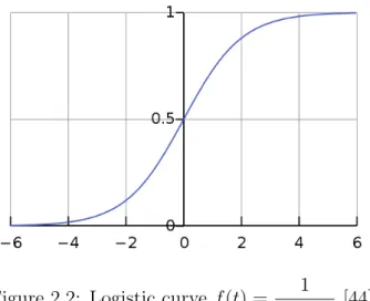
To introduce non-linearity into an ANN, we apply element-wise non-linear functions such as a sigmoid function or a rectified linear unit after linear projections. The non-linear function in each neuron is h=f(W x+b) where the non-linear mapping f acts as the activation function. The commonest activation function is sigmoid functionf(t) = 1

1 +e−t. We useσ() to represent

this sigmoid function. Thus each layer within an ANN consists a functionh =σ(W x+b), taking input x∈_Rd _{and mapping it to z ∈}

Rp.

Figure 2.2: Logistic curve f(t) = 1

2.2

Autoencoders

An autoencoder is an artificial neural network used for unsupervised learning of efficient codings. The aim of an autoencoder is to learn a representation (encoding) for a set of data, typically for the purpose of dimensionality reduction. Autoencoders are simple learning circuits which aim to transform inputs into outputs with the least possible amount of distortion. While conceptually simple, they play an important role in machine learning. Recently, autoencoders have taken center stage in the deep architecture approach and this concept has become more widely used for learning generative models of data [2, 4].

Figure 2.3: Schematic structure of an autoencoder with 3 fully-connected hidden layers [45].

Typically, an autoencoder consists two parts, an encoding phase (encoder)E(·) and an decoding phase (decoder)D(·). The encoderE(·) receives input data and outputs mid-layer-data, which acts as the input data for the decoder D(·). The decoder maps the mid-layer-data back to the original feature space. The encoder and decoder can be comprised of single layer or multiple layers, each layer with a functionz =σ(W x+b) mappingx∈_Rd_{toz ∈}

Rp. σis an element-wise activation function such as a sigmoid function or a rectified linear unit.

maps x ∈ _Rd _{= X to z ∈}

Rp = F (z is hidden layer, for this simplest case, it is also the mid-layer of the whole autoencoder). The encoder E(·) and the decoder D(·) can be defined as transitions φ and ψ. An autoencoder AE can be written in the following form:

φ :X → F ψ :F → X AEφ,ψ = argmin φ,ψ kX−ψ(φ(X))k2_F (2.3)

The encoder stage of the autoencoder maps xto a mid-layer z (usually in lower dimension):

z =σ(W x+b) (2.4)

The decoder stage of the autoencoder maps z to the reconstruction x0 of the same shape and in the same dimension with original data x:

x0 =σ0(W0z+b0) (2.5)

In the training process, autoencoders are usually trained to minimize reconstruction errors (such as squared errors) between original x and the reconstructedx0:

L(x, x0) =kx−x0k2 =kx−σ0(W0(σ(W x+b)) +b0)k2 (2.6)

where x is usually averaged over some input training set [2].

2.3

Canonical Correlation Analysis

In statistics, Canonical Correlation Analysis (CCA) is a way of inferring information from cross-covariance matrices. If we have two vectors X = (X1, ..., Xn) and Y = (Y1, ..., Ym) of

random variables, and there are correlations among the variables, then CCA will find linear combinations of the Xi and Yj which have maximum correlation with each other [13]. In this

Section, we are inspired by, and closely follow the notation and derivations, that can be found in Pezeshki and Scharf, 2004 [5].

Consider two random vectors x ∈ _Rm _{and y ∈}

Rn. Let z = h

xT _yTi T

that x and y have zero means and share the nonsingular composite covariance matrix Rzz =E[zzT] =   Rxx Rxy Rxy Ryy   (2.7)

where the elements of the cross-covariance matrix Rxy are inner products in the Hilbert space

of second-order random variables. Rxy[i, j] = E[xiyj] is the inner product between random

variables xi and yj in the Hilbert space.

The coherence matrix of x and y is defined as

C =E[(R_xx−1/2x)(R−_yy1/2y)T] =R_xx−1/2RxyRyy−T /2 (2.8)

A singular value decomposition (SVD) for the coherence matrix C may be written as

C =R−_xx1/2RxyR−yyT /2 =FΣG T_,

FTCG=FTR_xx−1/2RxyR−yyT /2G= Σ

(2.9)

whereF ∈_Rm×m_andG∈

Rn×nare orthogonal matrices and the matrix Σ is a diagonal singular value matrix with Σ(m) = diag[σ1, σ2, ..., σm]; σ1 ≥ σ2 ≥ ... ≥ σm > 0. Let the elements of

u∈_Rm _{and v ∈}

Rn be the canonical coordinates of xand y. The diagonal matrix

Σ =FTCG=FTR_xx−1/2RxyRyy−T /2G=E[(F T_R−1/2 xx x)(G T_R−T /2 yy y) T_{] =E[uv}T_{] (2.10)}

is the canonical correlation matrix. Each σi is the correlation between pairs of canonical

coordinates (ui, vi).

From the above equation, we extract the following expression for canonical variables u and v:

u=FTR−_xx1/2x, v =GTR−_yyT /2y (2.11)

The standard measure of linear dependence for the composite vector is the Hadamard ratio where the ratio takes the value 0 if and only if there is linear dependence among the elements of the composite vector and takes the value 1 if and only if elements of the composite vector are mutually uncorrelated.

In [5], the authors make a decomposition of the Hadamard ratio and derived the following term L=det(I−ΣΣT) = m Y i=1 (1−σ_i2); 0≤L≤1 (2.12)

which measures the linear dependence between xand y. Correspondingly,

H = 1−L= 1−det(I−ΣΣT) = 1− m

Y

i=1

(1−σ_i2); 0≤H ≤1 (2.13)

measures the linear coherence between x and y.

2.4

Kernel Methods

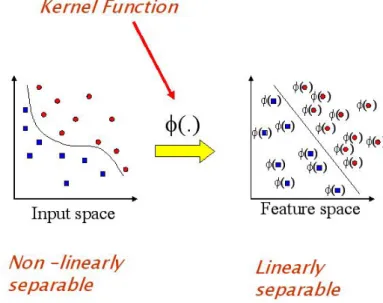
Kernel methods owe their name to the use of kernel functions, which enable them to operate in a high-dimensional, implicit feature space without ever computing the coordinates of the data in that space, but rather by simply computing the inner products between the images of all pairs of data in the feature space. This operation is often computationally cheaper than the explicit computation of the coordinates. This approach is called the “kernel trick” [18]. Given xi and yj, the function K(xi, yj) :R×R→R is often referred to a kernel function.

Figure 2.4: A visual demonstration of kernel function. A kernel function maps data from original feature space to a higher dimensional space and avoids the explicit mapping that is needed to get linear learning algorithms to learn a nonlinear function or decision boundary [42].

2.4.1

Positive Definite Kernel

A positive definite kernel is a generalization of a positive definite function or a positive definite matrix. It makes sure there is a corresponding inner product space for x and y. Its greatest advantage is that positive definite kernels can be defined on every set. Therefore it can be applied to data of any type.

Definition. [19] A kernel is a symmetric continuous function

K : [a, b]×[a, b]→_R (2.14)

where symmetric means that K(x, s) = K(s, x). K is said to be positive definite if and only if

n X i=1 n X j=1 K(xi, xj)cicj >0 (2.15)

The computation for kernel function K is made much simpler if the kernel can be written in the form of a ”feature map”ϕ:X → V which satisfiesK(x, x0) =hϕ(x), ϕ(x0)iV. However, the key restriction is thath·,·iV must be a proper inner product. While some problems in machine learning do require an explicit representation for ϕ, ϕis not necessary as long as V is an inner product space [19].

In KPCA or KCCA, a kernel function maps data from original space to an inner product space RKHS to ensure both the existence of an inner product and the evaluation of every function in this space at every point in the domain. From the definition of RKHS, the corresponding kernel function should be both symmetric and positive definite [10].

2.4.2

Schoenberg’s Theorem

Suppose a kernel function K is not positive definite, it may not represent an inner product in any Hilbert space. Here is one way to see. A kernel K is positive definite if and only if for all samples of n points, its corresponding kernel matrix K is a positive definite matrix. With a positive definite K, by Cholesky decompose K = LLT, each row of L is one mapped point in the inner product space. If K is not positive definite, the matrix K may also not be positive definite. Consequently, Cholesky does not work and there is no corresponding inner product space.

derivativesf(n)(x) for all n = 0,1,2,3, ...and if (−1)nf(n)(x)≥0 [21].

Schoenberg [22] provides a method to ensure the kernel function to be positive definite: Iff(t) is a completely monotonic function, then the radial kernel

K(x, y) = f(kx−yk2) (2.16)

is positive definite on any Hilbert space. Since the radial kernel is already symmetric, the above Schoenberg’s theorem provides us a direct way to get a symmetric positive definite kernel function satisfying RKHS definition for our model.

2.5

KCCA

In section 2.3, we explain CCA step by step. For two random vectors x ∈ Rm _{and y ∈ R}n_,

let z = hxT yT

iT

∈ Rm+n and assume that x and y have zero means. Formula 2.7 is the covariance matrix of x and y. The elements of the cross-covariance matrix Rxy are inner

products in Hilbert space of second-order random variables. Rxy[i, j] = E[xiyj] is the inner

product between random variables xi and yj in the Hilbert space. To leverage the power of

non-linearity, we apply kernel methods to CCA. As in the linear case, the aim of KCCA is to find canonical variables of the input data. Thus we derive its calculation based upon the formulas for CCA in section 2.3.

Here, to obtain the covariance matrix of xand y in RKHS, we define

Rxx[i, j] =K(xi, xj)

Rxy[i, j] =K(xi, yj)

Ryx[i, j] =K(yi, xj)

Ryy[i, j] =K(yi, yj)

(2.17)

becomes Rzz =   Rxx Rxy Rxy Ryy  =                    K(x1, x1) . . . K(x1, xm) .. . . .. K(xm, x1) K(xm, xm)           K(x1, y1) . . . K(x1, yn) .. . . .. K(xm, y1) K(xm, yn)           K(y1, x1) . . . K(y1, xm) .. . . .. K(yn, x1) K(yn, xm)           K(y1, y1) . . . K(y1, yn) .. . . .. K(yn, yn) K(yn, yn)                    (2.18)

where the elements of the cross-covariance matrix Rxy are inner products in the RKHS of

random variables x and y. Rxy[i, j] =K(xi, yj) is the inner product between random variables

xi and yj in the RKHS.

We mimic all the remaining formulas from 2.8 to 2.13, except that, with kernel methods, L and H now measure the non-linear dependence and non-linear coherence between x and y respectively.

2.6

Principal Component Analysis

Principal Component Analysis (PCA) is a popular unsupervised learning approach for discov-ering a low-dimensional set of features from a large set of variables. We rest our introduction to this algorithm upon the definitions in [17] and closely follow its organization. For high-dimensional data, principal components allow us to summarize this set with a smaller number of representative variables that collectively explain most of the variability in the original set. PCA refers to the process by which principal components are computed, and the subsequent use of these components in understanding the data. The first principal component of a set of features X = (X1, X2, ..., Xp) is the normalized linear combination of the features

that has the largest variance. The first principal component vector z1 solves the following optimization problem: minimize D0 D−D 0 F subject to rank(D 0 )≤r (2.20)

where D is data matrix and r is an desired rank. This can be solved via an eigen decomposition, a standard technique in linear algebra.

After the first principal component Z1 of the features has been determined, we can find the second principal component Z2. The second principal component is the linear combination of X = (X1, X2, ..., Xp) that has maximal variance out of all linear combinations that are

uncorre-lated withZ1. The third principal component is the linear combination ofX = (X1, X2, ..., Xp)

that has maximal variance out of all linear combinations that are uncorrelated withZ1 and Z2. So on and so forth.

Finally, we will have totally p unique principal components Z1, Z2, ..., Zp. Each unique

princi-pal component Zi explains a specific percentage of variance to the original dataset, a positive

quantity, ranging from 0 to 1. And the percentages of all p principal components sum to 1. In most programming PCA tools, the principal components appear with a descending order of the percentages by variance they explain. These percentages are cumulative, indicating the cumu-lative variance explained to the original dataset by their corresponding principal components. Thus, to understand the data and execute proceeding analysis after PCA, we typically extract first k principal componentsZ1, Z2, ..., Zk, k < p. These k principal components usually explain

Chapter 3

Model Design

In Section 2.1 and 2.2, we describe how autoencoders learn through training and finally recon-struct data x back to its original space with minimal reconstruction errors. Herein we modify this task: given an input data set x, we want our model to reconstruct another data set y. From initial experiments on autoencoders, we find that the reconstruction results are mediocre. Actually, an autoencoder does not have explicit training process to explore the dependency between two datasets x and y. Instead, it merely explores “direct mapping” from one cluster of patterns to another one. This leads to devastating issues in reconstruction results (In next Chapter, we will use some image examples to demonstrate this deficiency). To better accom-plish the new task, we introduce CCA and KCCA to explore the dependency between the pair of input data sets.

In this Chapter, we will introduce three models, the Non-Coherence Encoder (NCE), the Co-herence Encoder (CE) and the Kernel Coherence Encoder (KCE) as well as their theoretical details. NCE is designed without CCA and coherence. In this model, the connection between the two data sets is explored exclusively through deep learning. In CE, we apply linear CCA within its encoder phase which outputs linear canonical variables to the decoder phase. In KCE, the ultimate model of the thesis research, we substitute linear CCA with KCCA thus extending the encoder phase to a non-linear stage. Notably, the decoder phases for these three models have exactly the same structure.

3.1

Non-Coherence Encoder (NCE)

This Section is a general introduction to NCE. The flowchart in figure 3.1 provides a step-by-step description. The model is divided into two phases, the encoder phase, and the decoder phase. Though having a different structure from an autoencoder, it maintains its major properties: dimension reduction, non-linear mapping, and reconstruction error minimization. The encoder phase reduces the dimension of input data, while the decoder phase maps data back to their original spaces and finish the reconstruction.

Original Datasetx∈_Rn _{and y∈}

Rn PCA on x, obtaining k principal com-ponentszx ∈ Rk PCA on y, obtaining k principal com-ponentszy ∈ Rk

Linear neural network mapping zx to zy0 ∈ Rk.

PCA reconstruction on z_y0, obtaining y00 ∈ _Rn

Linear neural network mapping zy to zx0 ∈Rk. PCA reconstruction on z_x0, obtaining x00 ∈ _Rn Nonlinear encoder, obtaining recon-structed data y0 Nonlinear encoder, obtaining recon-structed data x0

evaluate the reconstruction results with proper metric Figure 3.1: Flowchart: Structure of NCE

3.1.1

Encoder Phase

The only step in the encoder phase of the model NCE is PCA. We reduce the dimension of the original data to a low-dimensional space where the principal components contain most information of the data.

PCA

In real-life problems, data x ∈ _Rn _{and y ∈}

Rn are usually high-dimensional, addressing the concern about computational efficiency, and moreover, over-fitting [17] that makes our model neither efficient nor effective. So we apply PCA to reduce the dimensions of original data. As we described in Chapter 2, PCA is a dimension reduction algorithm that allows us to summarize high-dimensional data set with a smaller number of representative variables that collectively explain most of the variability in the original set.

To reach a trade-off between model accuracy and the above two concerns, we take the first k principal components Z1, Z2, ..., Zk that explain over 90% variance of the original data, where

k is a much smaller integer compared with the original dimension n. As a result, the input data for the KCCA step become zx ∈ Rk and zy ∈ Rk. Meanwhile, we keep the eigenvectors and means of x and y generated in this step for PCA reconstruction.

3.1.2

Decoder Phase

The decoder phase of NCE maps zx toy0 and zy to x0 through three steps: linear ANNs, PCA

reconstruction, and non-linear ANNs. Linear ANNs

The first step for the decoder phase is to transferzxandzy to the spaces of principle components

zy and zx respectively. Here we use a pair of two-layer linear ANNs to map zx and zy to zy0

and zx0, namely γ1 and γ2:

z_y0 =W1,2(W1,1zx+b1,1) +b1,2 z_x0 =W2,2(W2,1zy+b2,1) +b2,2 γ1(W1,1, W1,2, b1,1, b1,2) = argmin W1,1,W1,2,b1,1,b1,2 zy−z 0 y 2 γ2(W2,1, W2,2, b2,1, b2,2) = argmin W2,1,W2,2,b2,1,b2,2 zx−z 0 x 2 (3.1) γ1 and γ2 provide us z 0 y and z 0

PCA Reconstruction

In PCA reconstruction step, the principal componentszxandzy are mapped back to the original

feature space of y and x with the following approach:

P CA reconstruction =P rincipal Components·EigenvectorsT +M ean (3.2)

Eigenvectors map the principal components z ∈_Rk _{back to the original feature space x}0

∈_Rn_.

In this step, we make use of the eigenvectors and means of y and xobtained in encoder phase:

y00 =z0_y·EigenvectorsT_y +M eany

x00 =z0_x·EigenvectorsT_x +M eanx

(3.3)

Non-linear ANNs

From experimental results, we find that the results of PCA reconstruction y00 and x00, though in the feature space of y and x, are not precise reconstruction. On the one hand, PCA re-construction amplifies training errors from _Rk to_Rn. On the other hand, since the k principal components explain about 90% variances, a small part of the information from the original data gets lost. For these two reasons, we need one more training step where the errors are computed in the feature spaces of original data sets.

This training process for our model is a pair of two-layer non-linear ANNs mappingy00toy0 and x00 tox0 respectively. It minimizes the error betweeny0 and original data y and error between x0 and original data x. We define the two ANNs asE1 and E2:

y0 =W1,3(W1,4y00+b1,3) +b1,4 x0 =W2,3(W2,4x00+b2,3) +b2,4 E1(W1,3, W1,4, b1,3, b1,4) = argmin W1,3,W1,4,b1,3,b1,4 ky−y0k2 E2(W2,3, W2,4, b2,3, b2,4) = argmin W2,3,W2,4,b2,3,b2,4 kx−x0k2 (3.4)

This is the last step of the whole model. Once the training errors converge, we obtain recon-struction y0 and x0 and evaluate the model performance.

3.2

Coherence Encoder (CE)

This Section is a general introduction to CE. The flowchart in figure 3.2 provides a stepwise description of the model. CE also has encoder phase and decoder phase. Comparing with NCE, the encoder phase contains CCA while the decoder phase remains the same.

Original Datasetx∈_Rn _{and y∈}

Rn PCA on x, obtaining k principal com-ponentszx ∈ Rk PCA on y, obtaining k principal com-ponentszy ∈ Rk CCA on zx, zy, obtaining canonical variables u, v

Linear neural network mapping u toz_y0 ∈ _Rk_.

PCA reconstruction on z_y0, obtaining y00 ∈ _Rn

Linear neural network mapping v toz_x0 ∈ _Rk_. PCA reconstruction on z_x0, obtaining x00 ∈ _Rn Nonlinear encoder, obtaining recon-structed data y0 Nonlinear encoder, obtaining recon-structed data x0

evaluate the reconstruction results with proper metric Figure 3.2: Flowchart: Structure of CE

3.2.1

Encoder Phase

In the encoder phase of CE, we apply linear CCA to extract the connection between the two data sets. More precisely, CCA is done with the principal components of the original data.

PCA

The PCA step is exactly the same with the encoder phase of NCE. It takes original datax∈_Rn

and y∈_Rn _{and generates their principal components z}

x ∈Rk and zy ∈Rk.

CCA

In this step, CE extracts correlation between two sets of principal components by linear CCA. Here we obtain the canonical variables u and v corresponding to zx and zy.

The calculation is based upon formulas in Section 2.3. Given principal components zx ∈ Rk

and zy ∈Rk. Let z =

h

zT x zyT

iT

∈_R2k_{. We obtain the following covariance matrix}

Rzz =E[zzT] =   Rzxzx Rzxzy Rzxzy Rzyzy   (3.5)

Then, with formulas 2.8 to 2.11, we get the canonical variables u and v,

u=FTR−_xx1/2x, v =GTR−_yyT /2y (3.6)

3.2.2

Decoder Phase

As we mentioned earlier, the decoder phase of CE shares exactly the same structure with the decoder phase of NCE. The only difference is that here we take canonical variables u and v as the input of the decoder phase.

z_y0 =W1,2(W1,1u+b1,1) +b1,2 z_x0 =W2,2(W2,1v+b2,1) +b2,2 γ1(W1,1, W1,2, b1,1, b1,2) = argmin W1,1,W1,2,b1,1,b1,2 zy−z 0 y 2 γ2(W2,1, W2,2, b2,1, b2,2) = argmin W2,1,W2,2,b2,1,b2,2 zx−z 0 x 2 (3.7)

3.3

Kernel Coherence Encoder (KCE)

Based on the ideas of autoencoder and linear CCA, we built CE. In KCE we extend the traditional CCA from linear to non-linear by kernel methods and increase the performance of CCA in a similar way by leveraging the non-linear capabilities of autoencoders. The flowchart in figure 3.3 provides a stepwise description of KCE.

Original Datasetx∈_Rn _{and y∈} Rn PCA on x, obtaining k principal com-ponentszx ∈ Rk PCA on y, obtaining k principal com-ponentszy ∈ Rk KCCA on zx, zy, obtaining kernel function K(zx, zy) and canonical variables u, v

Linear neural network mapping u toz_y0 ∈ _Rk_.

PCA reconstruction on z_y0, obtaining y00 ∈ _Rn

Linear neural network mapping v toz_x0 ∈ _Rk_. PCA reconstruction on z_x0, obtaining x00 ∈ _Rn Nonlinear encoder, obtaining recon-structed data y0 Nonlinear encoder, obtaining recon-structed data x0

evaluate the reconstruction results with proper metric Figure 3.3: Flowchart: Structure of KCE

3.3.1

Encoder Phase

In the encoder phase of KCE, we apply KCCA to extract the nonlinear dependency between the two datasets. More precisely, KCCA is done with the principal components of the original data.

PCA

The PCA step is exactly the same with the encoder phase of NCE. It takes original datax∈_Rn

and y∈_Rn _{and generates their principal components z}

x ∈Rk and zy ∈Rk.

In this step, we are supposed to train an optimal kernel function that maximizes the coherence between the pair of principal components zx and zy and obtain the canonical variables uand v

corresponding to zx and zy.

To ensure that for any scalarzx,i inzx = (zx,1, zx,2, ..., zx,k) andzy,j inzy = (zy,1, zy,2, ..., zy,k) the

kernel functionK(zx,i, zy,j) always represents an inner product in the Hilbert space, this kernel

function has to be positive definite. One way to satisfy this constraint is to apply Schoenberg’s theorem: if f(t) is a completely monotonic function, then the radial kernel K(zx,i, zy,j) =

f(kzx,i−zy,jk2) is positive definite on any Hilbert space. We use one of the simplest completely

monotonic function

f(t) =e−αt+β, α >0 (3.8) K(zx,i, zy,j) =e−αkzx,i−zy,jk

2_+β

(3.9) To maximize the non-linear coherence of the input pair of data, we set non-linear dependence as the cost function in the training process. Summarizing [5], we extract the following formulas in Chapter 2. L and H represent nonlinear dependence and coherence between zx and zy.

L=det(I−ΣΣT) = m Y i=1 (1−σ_i2); 0≥L≥1 (3.10) L= det(Rzz) det(Rzxzx)det(Rzyzy) = det     Rzxzx Rzxzy Rzyzx Rzyzy     det(Rzxzx)det(Rzyzy) (3.11) H = 1−L= 1− det     Rzxzx Rzxzy Rzyzx Rzyzy     det(Rzxzx)det(Rzyzy) (3.12) One problem of the above formulas is that they are sensitive to high-dimensional space. If one σi is large, the result of dependence formula tends to 0 and coherence tends to 1. As a result,

the coherence between zx and zy tends to small if anyzx is predictable for any zy or any zy is

predictable for anyzx. On the other hand, the high-dimensional covariance matrix can be close

to singular and makes it difficult to compute determinant, as is required by using a coherence metric. Here we propose a novel element-wise modification to the calculation of dependence

and coherence to avoid above issues: Li,j = det    

Rzx,izx,i Rzx,izy,j

Rzy,jzx,i Rzy,jzy,j



 



det(Rzx,izx,i)det(Rzy,jzy,j)

= Rzx,izx,iRzy,jzy,j −Rzx,izy,jRzy,jzx,i

RzxzxRzyzy

(3.13)

Li,j represents the element-wise dependence between zx,i and zy,j. Now we have

L= Pk i,j=1(Li,j)2 n2 (3.14) C = 1−L= 1− Pk i,j=1(Li,j) 2 n2 (3.15)

By our new formula, the novel coherence C is small if and only if all zx is predictable from zy

and all zy is predictable from zx. As a result, in the encoder phase of KCE, the connection

betweenx and y comes only from the element-wise coherence betweenzx andzy in the RKHS.

We define κ as the kernel function training process

κ= argmin

α,β

L (3.16)

Once the cost converges to a small value, we obtain the parameters α and β and the corre-sponding optimal kernel function K(zx,i, zy,j) = e−αkzx,i−zy,jk

2_+β

.

The representation of Rzz follows formula 2.18 while the remaining calculation of canonical

variables u and v follows formulas 2.8 to 2.11.

3.3.2

Decoder Phase

The decoder phase of the KCE shares exactly the same structure with the decoder phases of the other two models.

Chapter 4

Numerical Results

In this Chapter, we demonstrate the effectiveness of our proposed models using the well-known image recognition MNIST data set. With some proper quantitative metrics, we will evaluate the reconstruction images by NCE, CE, and KCE.

4.1

Data Sets

MNIST data set [39] is a classical data set widely used for machine learning and deep learning study, especially in image processing and pattern recognition problems. With feature data (pixel values of images) and labels provided, it can be used for both supervised and unsupervised learning. The data set contains 55000 images for training and 10000 images for testing. Each image is a 28×28 pixel picture of a human hand-written digit (0-9) one 0-to-1 grayscale canvas with the pure black background (pixel value 0.0) and pure white writing (pixel value 1.0).

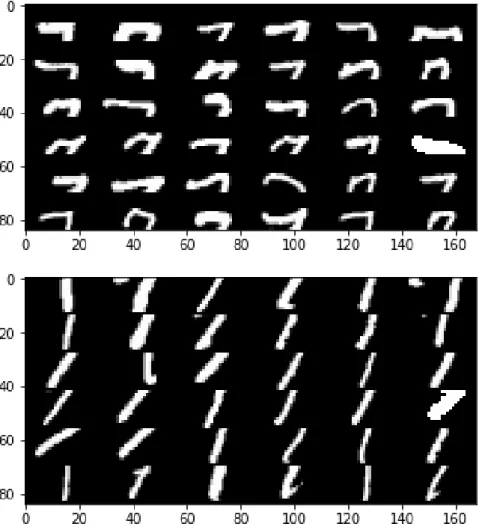
To fit our model design, we need a pair of data sets with some correlations in between. Our strategy is to cut each image (784 pixels) to upper and lower parts with equal sizes (14×28), as shown in Figure 4.2. The upper parts of the images are xand the lower parts of the images are y. In this circumstance, features inx and y are dependent on each other.

Given the labels indicating the digit, we group the images by their labels thus each group contains images corresponding to only one digit. We test our model for each group separately where images share similar features and patterns of that digit. This is to ensure the strength of dependency between two data sets.

Figure 4.2: 36 examples of upper and lower parts of digit 7 images.

The experimental result indicates that the first 10 principal components explain more than 90% variance of the original image data. Thus we set k= 10 for PCA.

4.2

Implementation Detail

4.2.1

TensorFlow

TensorFlow [14, 15] is an open source software library for numerical computation using data flow graphs, a machine learning system that operates at large scale and in heterogeneous envi-ronments. It comes with strong support for machine learning and deep learning and the flexible numerical computation core is used across many other scientific domains. This system gives great flexibility to the application developer and enables developers to experiment with novel optimizations and training algorithms. In Chapter 3, we mention a kernel function optimization training κ (3.15), linear ANNS γ (3.1) and non-linear ANNs E (3.4). These pieces of training are implemented on TensorFlow.

Figure 4.3: A schematic TensorFlow dataflow graph for a training pipeline, containing sub-graphs for reading input data, preprocessing, training, and checkpointing state [46].

4.2.2

Gradient Descent Optimization

Gradient descent optimization [29] is one of the most popular algorithms to perform optimiza-tion and by far the most common way to optimize artificial neural networks. Here we briefly introduce one of the variants of gradient descent, batch gradient descent, which is applied by TensorFlow classtf.train.GradientDescentOptimizer [28]. In code, batch gradient descent looks something like this:

f or i in range(# epochs) :

params grad =evaluate gradient(cost f unction, data, params) params =params−learning rate∗params grad

For example, for the following optimization φ with parameters W and b, h=f(W x+b) cost=kx−x0k₂ φ= argmin W,b cost (4.2)

In each step (epoch) i, batch gradient descent computes the gradient of the cost function with respect to the parameters for the entire training dataset:

G(Wi) = ∂ cost ∂ h ∂ h ∂f(Wi) ∂f(Wi) dWi G(bi) = ∂ cost ∂ h ∂ h ∂f(bi) ∂f(bi) dbi Wi+1 =Wi−αG(Wi) bi+1 =bi−αG(bi) (4.3)

where α refers to learning rate and G() refers to the gradient of a parameter. In TensorFlow implementation, we can use a one-line code

optimizer = tf.train.GradientDescentOptimizer(learning rate).minimize(cost)

4.2.3

Training Parameters

We set the training parameters for all training processes in the models:

hidden layer dimension = 100, learning rate = 0.01,

training epochs = 2000, batch size = 100

Based on experiments, we conclude that these parameters make sure all the steps can be well trained. For a fair comparison, we keep the parameters consistent in all models.

4.3

Evaluation Metrics

To evaluate the reconstruction results, we specify multiple metrics. For image data, for example, the most direct way to check reconstruction performance is to convert the output data back to original canvas size and print the image with reshaped data. Then we can evaluate the

reconstruction visually by comparing the reconstruction image with original image. Usually, this is a very effective approach. However, it is not guaranteed that human eyes are able to identify all trivial differences between two images, and it is hard to claim which model works better if two models output similar reconstruction images, or demonstrate visually indistinguishable levels of performance. Thus it is necessary to introduce some quantitative measures.

Our purpose here is to compare the reconstructed image data and original image data by quan-tifying the error, the distance or the similarity between them. This is equivalent to the Image Similarity Analysis [30, 31, 34]. We apply 5 different metrics: L2_{-norm [32], Pearson} Correla-tion score [30], cross-correlaCorrela-tion [34], Bhattacharyya distance [31] and Fast Fourier Transform (FFT) rank [31].

4.3.1

L

-Norm

For real vectors x= [x1, x2, ...xn],L2-Norm [32] is given by

kxk₂ = v u u t n X i=1 x2 i (4.4)

TheL2-Norm is also known as the Euclidean norm because it measures the distance in Euclidean space. For output data vectorx0andy0, we can measure their reconstruction error by calculating L2-Norm of x−x0 and y−y0 respectively.

kx−x0k₂ = v u u t n X i=1 (xi−x0i)2 ky−y0k₂ = v u u t n X i=1 (yi−y0i)2 (4.5)

Note that L2-Norm works for data as vectors. After reshaping the data to matrix form, the measure turns to Frobenius norm [32]. But the result will not change.

4.3.2

Pearson Correlation Score

Pearson Correlation Coefficient [30, 33] is a measure of the linear correlation between two variables x and y. It has a value between -1 and +1, where 1 indicates total positive linear correlation, 0 is no linear correlation, and 1 is the total negative linear correlation. Accordingly,

Pearson Correlation score measures how highly correlated are two variables. A score of 1 indicates that the data objects are perfectly correlated but in this case, a score of -1 means that the data objects are not correlated. In other words, the Pearson Correlation score quantifies how well two data objects fit a line.

In essence, the Pearson Correlation score finds the ratio between the covariance and the standard deviation of both objects. In our case, we calculate the Pearson Correlation score between x and x0, y and y0 as the following:

P earson(x, x0) = P xx0− P xP x0 n r (P x2₋( P x)2 n )( P x02₋ ( P x0)2 n ) P earson(y, y0) = P yy0− P yP y0 n r (P y2₋ ( P y)2 n )( P y02₋ ( P y0)2 n ) (4.6)

Since the model generates data in the same scale with input data, a larger Pearson Correlation score here refers to greater similarity, thus better reconstruction result.

4.3.3

Cross-correlation

In signal processing, cross-correlation [34] is a measure of similarity of two series as a function of the displacement of one relative to the other. This measure has been used in medical image registration. For 1-dimensional data, this approach is essentially same as Pearson correlation coefficient score method:

CC(x, x0) = Pn i=1(xi−x)(x 0 i−x0) npvar(x)var(x0₎ CC(y, y0) = Pn i=1(yi−y)(y0i−y0) npvar(y)var(y0₎ (4.7)

However, for 2-dimensional data, this measure has one advantage: it takes care of the data shifting just like cross-correlation method takes care of the time-delay between signals in signal processing. In our case, let c2d() represents 2-dimensional cross-correlation computation, for

the reshaping data x, y, x0, y0 ∈_Rm×n_, CC2dx =c2d( x−x p var(x), x0−x0 p var(x0₎)/(m·n) CC2dy =c2d( y−y p var(y), y0−y0 p var(y0₎)/(m·n) (4.8)

HereCC2dx and CC2dy are two arrays containing cross-correlation coefficients (range -1 to 1)

in different phases. We select the maximum values of them to represent the similarity between x and x0 and between y and y0 respectively.

4.3.4

Bhattacharyya Distance

In statistics, the Bhattacharyya distance [31, 35, 36] measures the similarity of two discrete or continuous probability distributions. In image processing, this measure can be used to determine the relative closeness of the two samples being considered. In our case [31],

d(x, x0) = v u u t1− 1 √ xx0_n2 n X i=1 p xix0i d(y, y0) = v u u t1− 1 p yy0_n2 n X i=1 p yiy0i (4.9)

A zero Bhattacharyya distance means that two data are exactly the same. Larger Bhat-tacharyya distance refers to greater gap or difference between them.

4.3.5

FFT Rank

Fourier transform [37] is an important image processing tool which is used to transform an image from the spatial domain into frequency domain. A Fast Fourier transform (FFT) [38] reduces the complexity of Fourier transform from N2 _{to N logN. This major improvement of} computational makes FFT practically possible in many applications. FFT is an algorithm that samples a signal (or signal-like data) over a period of time (or space) and transforms it into its frequency domain. In the frequency domain, each point represents a particular frequency contained in the spatial domain. The points in frequency domain have both real and imaginary parts, which represent magnitude and phase respectively. In our evaluation of reconstruction, we use only the real part (magnitude) of the FFT results, as it contains most of the information

of original data in the spatial domain.

In our case, we use the following rank formula as our metric for comparison. Here x, y, x0, y0 refer to intensity values of data (data in spatial domain), and Fx, Fy, Fx0, F_y0 represent the

average frequency values of them (in frequency domain) [31].

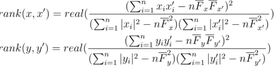
rank(x, x0) = real( ( Pn i=1xix0i−nFxFx0)2 (Pn i=1|xi|2−nF 2 x)( Pn i=1|x 0 i|2−nF 2 x0) ) rank(y, y0) =real( ( Pn i=1yiy 0 i −nFyFy0)2 (Pn i=1|yi|2−nF 2 y)( Pn i=1|y 0 i|2−nF 2 y0) ) (4.10)

A rank ranges from -1 to 1, where 1 is obtained if two datasets are exactly the same and -1 if they are fully independent from each other. The higher the rank, the more similarity shared by the two datasets.

4.4

Reconstruction Images

4.4.1

Simple ANNs Reconstruction

Our initial trial for reconstruction is running a pair of non-linear ANNs on the MNIST data sets. This is a simulation of the autoencoders. The neural networks, with one data set as input, are trained to minimize the difference between reconstructed data and the other data set. Consequently, the model builds maps between two dependent data sets.

Original Datasetx∈_Rn _{and y∈}

Rn

2-layer neural ar-tifical network, mapping x toy0

2-layer neural ar-tifical network, mapping y tox0

evaluate the reconstruction results with proper metric

Figure 4.4: Flowchart of the simple paired ANNs. We initially design this model to work like “paired autoencoders”.

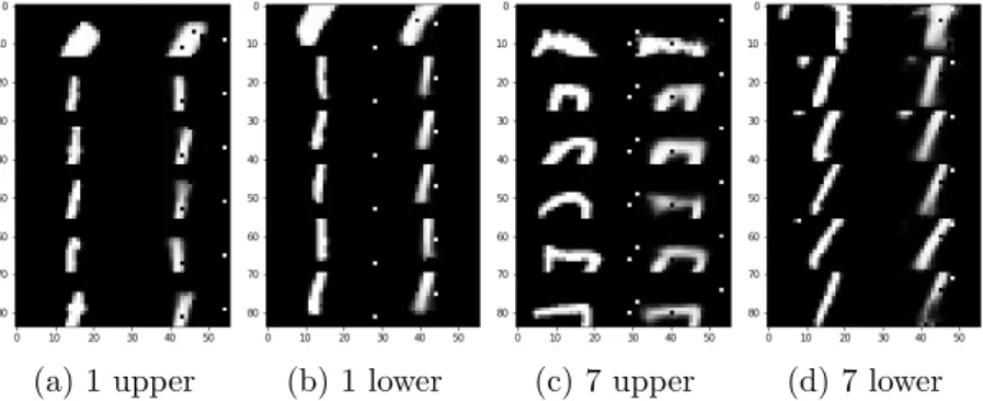
the ANNs is comprised of two non-linear layers following the classical activation function h= σ(W x+b). Below are some examples of the reconstruction images (we randomly select 6 hand-written images for each digit. The left part of a picture contains original digit images and the right part contains reconstructed images). Although the ANNs reconstruct most of the patterns for these images, it is notable that some abnormal white pixels in black background impact overall reconstruction quality. And the positions of these pixels are exactly the same in the samples of each digit. These flaws originate from the fact that ANNs learn and “memorize” a map between the two datasetsxandy, preventing the reconstruction from perfect. We call this issue “black-to-white” mapping errors. It is an interesting and meaningful theoretical question to explore [40], but here we are not going to discuss it now.

(a) 1 upper (b) 1 lower (c) 7 upper (d) 7 lower

4.4.2

NCE, CE and KCE Reconstruction

Digit KCE Upper KCE Lower CE Upper CE Lower NCE Upper NCE Lower

0

1

2

3

5

6

7

8

9

In the above table, we post all testing reconstruction results by the three well-trained models, KCE, CE and NCE. In this part, we randomly select 6 hand-written images for each digit from test data set and run all three models on these samples. The left part of a picture contains original digit images and the right part contains reconstructed images.

demon-strate the effectiveness of KCCA compared with linear CCA and non-CCA in our task. Since the decoder phases are identical within all three models, the reconstruction results can reflect the effectiveness of the encoder phase, more specifically, KCCA, CCA or neither.

From the table, we first compare the performance of the models visually. Contrasting the results from CE with the results from NCE, it is obvious that KCE generates better reconstruction. This is a convincing clue to claim the effectiveness of linear CCA. On the other hand, with CCA approach, the model solves the “black-to-white” mapping problem. Then we compare KCE with CE where the differences are not as easily observable. The patterns of hand-written digits are generally reconstructed in both models. However, the patterns of some reconstructed images from CE, such as upper part of 5 and lower part of 4 are smashed to pieces while this never occurs in KCE reconstruction. To authenticate the difference, we take a further step to quantitative metrics.

4.5

Quantitative Comparison

We use the 5 metrics for Image Similarity Analysis introduced in Section 4.3 to quantitatively evaluate the performances of our three models. For each model, we have 6 pairs of reconstructed image data sets for each digit 0-9, thus 120 arrays of data with size 392 (28×14), the total pixel number for one half-image. We do the image similarity analysis for KCE, CE, and NCE by comparing their reconstructed data with the original data to indicate the closeness of reconstruction. For each one of the metric, we calculate the mean of 120 scores/distances/ranks of the three models separately. Then we do T-tests [41] to compare KCE with CE and NCE respectively. We extract p-values indicating the confidence to claim that scores/distances/ranks are different (the smaller the p-value, the more confident to claim this). The statistical analysis results are shown in Table 4.1 and Table 4.2.

Metric NCE average KCE average p-value

2-norm 8.3188 4.94215 4.15186e-37

Pearson Coefficient 0.295733 0.618759 2.35119e-32

cross correlation 0.344092 0.712149 5.46184e-61

Bhattacharyya distance 0.693693 0.505529 2.48646e-33

FFT 0.204558 0.4972 2.14213e-30

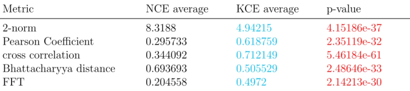
Table 4.1: Statistical results between KCE and NCE: the light blue highlights indicate better performance between KCE and NCE while the red highlights indicate p-value less than 0.05. The 5 metrics all demonstrate better performance to KCE with p-values lower than 0.05. we claim that KCE generates better reconstruction results than NCE.

Metric CE average KCE average p-value

2-norm 5.41653 4.94215 0.00297353

Pearson Coefficient 0.550588 0.618759 0.00663332

cross correlation 0.689174 0.712149 0.113121

Bhattacharyya distance 0.539608 0.505529 0.0272345

FFT 0.42421 0.4972 0.00352892

Table 4.2: Statistical results between KCE and CE: the light blue highlights indicate better performance between KCE and CE while the red highlights indicate p-value less than 0.05. Since all metrics point to the greater similarity between KCE reconstruction and original data and most p-values are less than the confidence threshold 0.05, we claim that KCE generates better reconstruction results than CE.

In general, from the statistics provided in the tables, KCE has greater performance than NCE and CE. Meanwhile, most of (9/10) the p-values are less than 0.05, small enough to support this claim. This further proves the effectiveness of KCCA over CCA and Non-CCA for our reconstruction task.

Chapter 5

Conclusion

5.1

Contribution

In this research, we propose three models to find complex correlations between two variables and KCE model demonstrates the best performance on a high dimensional image reconstruction task. Given two dependent high-dimensional data sets, KCE successfully builds a map between the two data sets. Thus we can reconstruct one data set by the other one. Our research starts with exploration on the limitation of CCA on high dimensional data through several experiments. In addition, with the help of Mercer’s theorem and Schoenberg’s theorem, we improve CCA by introducing kernel methods that map data to an RKHS. Meanwhile, we propose an element-wise modification of coherence calculation. In the processes of mapping canonical variables to the original feature space of another data set, we try both linear and non-linear ANNs and demonstrate that a non-linear ANN before PCA reconstruction and a non-non-linear ANN after PCA reconstruction best fit our requirements. CE and KCE both solve the “black-to-white” mapping error problem for grayscale image reconstruction. With 5 quantitative metrics, we prove the great effectiveness of KCCA in our paired reconstruction task.

5.2

Future Work

We propose three directions for the future work:

First, we believe that during the PCA projection, some information of original data gets lost. We will run more experiments to explore the dimensionality trade-off for better reconstruction results.

Second, we have observed that our model is able to avoid the “black-to-white” mapping error problem. It is worth exploring its reason and continuing to produce a mathematical proof. Third, so far we have only done the experiments on MNIST data. We should explore more samples including face images, item images or even other types of data to justify the effectiveness of our proposed model KCE.

Bibliography

[1] Lai, Pei Ling, and Colin Fyfe. ”Kernel and nonlinear canonical correlation analysis.” Inter-national Journal of Neural Systems10.05 (2000): 365-377.

[2] Tan, Chun Chet. Autoencoder neural networks: A performance study based on image reconstruction, recognition and compression.LAP Lambert Academic Publishing, 2009.

[3] aymericdamien, TensorFlow-Examples, (2017), GitHub repository,

https://github.com/aymericdamien/TensorFlow-Examples

[4] Baldi, Pierre. ”Autoencoders, unsupervised learning, and deep architectures.” Proceedings of ICML Workshop on Unsupervised and Transfer Learning. 2012.

[5] Pezeshki, A., Scharf, L. L., Azimi-Sadjadi, M. R., & Lundberg, M. (2004, November). Empirical canonical correlation analysis in subspaces. In Signals, Systems and Computers, 2004. Conference Record of the Thirty-Eighth Asilomar Conference on (Vol. 1, pp. 994-997). IEEE.

[6] Wold, Svante, Kim Esbensen, and Paul Geladi. ”Principal component analysis.” Chemo-metrics and intelligent laboratory systems 2.1-3 (1987): 37-52.

[7] Pearson, K. (1901). ”On Lines and Planes of Closest Fit to Systems of Points in Space”.

Philosophical Magazine. 2 (11): 559572.

[8] amoeba (https://stats.stackexchange.com/users/28666/amoeba), How to reverse PCA and reconstruct original variables from several principal components?, URL (version: 2016-08-12): https://stats.stackexchange.com/q/229092

[9] Autoencoder Using Kernel Methods http://technodocbox.com/3D Graphics/66255915-Autoencoder-using-kernel-method.html

[10] Gretton, Arthur. ”Introduction to rkhs, and some simple kernel algorithms.” Adv. Top. Mach. Learn. Lecture Conducted from University College London (2013): 16.

[11] Gram matrix. Encyclopedia of Mathematics.

URL:http://www.encyclopediaofmath.org/index.php?title=Gram matrix&oldid=35177

[12] Weisstein, Eric W. ”Singular Matrix.” From MathWorld–A Wolfram Web Resource.

http://mathworld.wolfram.com/SingularMatrix.html

[13] Hrdle, Wolfgang; Simar, Lopold (2007). ”Canonical Correlation Analysis”. Applied Mul-tivariate Statistical Analysis. pp. 321330. doi:10.1007/540-72244-1 14. ISBN 978-3-540-72243-4.

[14] Abadi, Martn, et al. ”TensorFlow: A System for Large-Scale Machine Learning.” OSDI. Vol. 16. 2016.

[15] ”Credits”. TensorFlow.org. Retrieved November 10, 2015. [16] ”TensorFlow Release”. Retrieved February 28, 2018.

[17] James, Gareth, et al. An introduction to statistical learning.Vol. 112. New York: springer, 2013.

[18] Theodoridis, Sergios (2008). Pattern Recognition. Elsevier B.V. p. 203. ISBN 9780080949123.

[19] Hein, Matthias, and Olivier Bousquet. ”Hilbertian metrics and positive definite kernels on probability measures.”AISTATS. 2005.

[20] Mercer, J. (1909), ”Functions of positive and negative type and their connection with the theory of integral equations”, Philosophical Transactions of the Royal Society A, 209 (441458): 415446

[21] Miller, Kenneth S., and Stefan G. Samko. ”Completely monotonic functions.” Integral Transforms and Special Functions 12.4 (2001): 389-402.

[22] Schoenberg Ann. of Math. textit39 (1938), 811-841)

[24] Schmidhuber, Jrgen. ”Deep learning in neural networks: An overview.” Neural networks 61 (2015): 85-117.

[25] Wang, Sun-Chong. ”Artificial neural network.” Interdisciplinary computing in java pro-gramming. Springer, Boston, MA, 2003. 81-100.

[26] Maxwell, Scott E., Harold D. Delaney, and Ken Kelley. Designing experiments and ana-lyzing data: A model comparison perspective.Routledge, 2017.

[27] Schlkopf, Bernhard, Alexander Smola, and Klaus-Robert Mller. ”Nonlinear component analysis as a kernel eigenvalue problem.”Neural computation 10.5 (1998): 1299-1319.

[28] Tensorflow Class GradientDescentOptimizer,

URL:https://www.tensorflow.org/api docs/python/tf/train/GradientDescentOptimizer

[29] Ruder, Sebastian. ”An overview of gradient descent optimization algorithms.” arXiv preprint arXiv:1609.04747 (2016).

[30] Segaran, Toby. Programming Collective Intelligence: Building Smart Web 2.0 Applications.

Sebastopol, CA: O’Reilly Media, 2007.

[31] Narayanan, Siddharth, and P. K. Thirivikraman. ”IMAGE SIMILARITY USING FOURIER TRANSFORM.”Journal Impact Factor 6.2 (2015): 29-37.

[32] Gradshteyn, I. S. and Ryzhik, I. M. Tables of Integrals, Series, and Products, 6th ed. San Diego, CA: Academic Press, pp. 1114-1125, 2000.

[33] ”SPSS Tutorials: Pearson Correlation”. Retrieved 2017-05-14.

[34] Avants, Brian B., et al. ”Symmetric diffeomorphic image registration with cross-correlation: evaluating automated labeling of elderly and neurodegenerative brain.”Medical image analysis 12.1 (2008): 26-41.

[35] Bhattacharyya, A. (1943). ”On a measure of divergence between two statistical populations defined by their probability distributions”.Bulletin of the Calcutta Mathematical Society.

[36] Guorong, Xuan, Chai Peiqi, and Wu Minhui. ”Bhattacharyya distance feature selection.”

Pattern Recognition, 1996., Proceedings of the 13th International Conference on. Vol. 2. IEEE, 1996.

[37] Bracewell, Ronald Newbold, and Ronald N. Bracewell. The Fourier transform and its applications.Vol. 31999. New York: McGraw-Hill, 1986.

[38] Bergland, G. D. ”A Guided Tour of the Fast Fourier Transform.”IEEE Spectrum 6, 41-52, July 1969.

[39] Tensorflow Digit Dataset https://www.tensorflow.org/get started/mnist/beginners

[40] Zhang, Chiyuan, et al. ”Understanding deep learning requires rethinking generalization.”

arXiv preprint arXiv:1611.03530(2016).

[41] Devore, Jay, Nicholas Farnum, and Jimmy Doi. Applied statistics for engineers and scien-tists. Nelson Education, 2013.

[42] Picture resource by Bioinformatics Lab, ICGEB, New Delhi,

http://bioinfo.icgeb.res.in/lipocalinpred/algorithm.html

[43] Picture resource by Glosser.ca - Own work, Derivative of File:Artificial neural network.svg, CC BY-SA 3.0,https://commons.wikimedia.org/w/index.php?curid=24913461

[44] Picture resource by Qef (talk) - Created from scratch with gnuplot, Public Domain,

https://commons.wikimedia.org/w/index.php?curid=4310325

[45] Picture resource by Chervinskii - Own work, CC BY-SA 4.0,

https://commons.wikimedia.org/w/index.php?curid=45555552

[46] Picture resource by Abadi, Martn, et al. ”TensorFlow: A System for Large-Scale Machine Learning.” OSDI. Vol. 16. 2016.

[47] Picture resource by Cheng, Chunling, et al. ”A multilayer improved RBM network based image compression method in wireless sensor networks.”International Journal of Distributed Sensor Networks 12.3 (2016): 1851829.