Cun Mu
Submitted in partial fulfillment of the requirements for the degree
of Doctor of Philosophy
in the Graduate School of Arts and Sciences
COLUMBIA UNIVERSITY
Structured Tensor Recovery and Decomposition
Cun Mu
Tensors, a.k.a. multi-dimensional arrays, arise naturally when modeling higher-order objects and relations. Among ubiquitous applications including image processing, collaborative filtering, demand forecasting and higher-order statistics, there are two recurring themes in general: tensor recovery and tensor decomposition. The first one aims to recover the underlying tensor from incomplete information; the second one is to study a variety of tensor decompositions to represent the array more concisely and moreover to capture the salient characteristics of the underlying data. Both topics are respectively addressed in this thesis.
Chapter2and Chapter3focus on low-rank tensor recovery (LRTR) from both theoretical and algorithmic perspectives. In Chapter2, we first provide a negative result to the sum of nuclear norms (SNN) model— an existing convex model widely used for LRTR; then we propose a novel convex model and prove this new model is better than the SNN model in terms of the number of measurements required to recover the underlying low-rank tensor. In Chapter3, we first build up the connection between robust low-rank tensor recovery and the compressive principle component pursuit (CPCP), a convex model for robust low-rank matrix recovery. Then we focus on developing convergent and scalable optimization methods to solve the CPCP problem. In specific, our convergent method, proposed by combining classical ideas from Frank-Wolfe and proximal methods, achieves scalability with linear per-iteration cost.
Chapter4generalizes the successive rank-one approximation (SROA) scheme for matrix eigen-decomposition to a special class of tensors called symmetric and orthogonally decomposable (SOD) tensor. We prove that the SROA scheme can robustly recover the symmetric canonical decomposition of the underlying SOD tensor even in the presence of noise. Perturbation bounds, which can be regarded as a higher-order generalization of the Davis-Kahan theorem, are provided in terms of the noise magnitude.
List of Figures iii
Notation iv
1 Introduction 1
1.1 Overview. . . 2
1.2 Notations and Preliminaries . . . 3
2 Low-Rank Tensor Recovery 12 2.1 Introduction . . . 12
2.2 Bounds for Non-Convex Recovery . . . 14
2.3 Convexification: Sum of Nuclear Norms? . . . 16
2.3.1 General lower bound for multiple structures . . . 17
2.3.2 Low-rank tensors . . . 23
2.4 A Better Convexification: Square Deal . . . 25
2.5 Tensor denoising . . . 28
2.6 Proofs for Section 2.2 . . . 30
2.7 Proofs for Section 2.3 . . . 33
2.8 First-Order Methods for Problems (2.3.22) and (2.4.5) . . . 35
2.8.1 Dykstra’s Algorithm for problem (2.3.22) . . . 35
2.8.2 Douglas-Rachford Algorithm for problem (2.4.5). . . 36
2.9 Conclusion . . . 37
3 Robust Low-Rank Tensor Recovery 39 3.1 Robust Low-Rank Matrix Recovery . . . 40
3.2 Preliminaries on Frank-Wolfe method . . . 42
3.3 Frank-Wolfe-Projection Method for Norm Constrained Problem . . . 48
3.3.1 Frank-Wolfe for problem (3.3.1) . . . 49
3.3.2 FW-P algorithm: combining Frank-Wolfe and projected gradient . . . 51
3.4 Frank-Wolfe-Thresholding Method for Penalized Problem. . . 52
3.4.1 Reformulation as smooth, constrained optimization . . . 53
3.4.2 Frank-Wolfe for problem (3.4.6) . . . 55
3.4.3 FW-T algorithm: combining Frank-Wolfe and proximal methods. . . 57
3.5 Numerical Experiments . . . 62
3.5.1 ISTA & FISTA for problem (3.1.5) . . . 63
3.5.2 Foreground-background separation in surveillance video . . . 65
3.5.3 Shadow and specularity removal from face images . . . 65
3.6 Discussion . . . 66
4 Successive Rank-One Approx. for Nearly Orthogonally Decomposable Symmetric Tensors 71 4.1 Introduction . . . 71
4.2 Rank-One Approximation . . . 76
4.2.1 Review of matrix perturbation analysis . . . 77
4.2.2 Single rank-one approximation . . . 78
4.2.3 Numerical verifications for Theorem 4.2 . . . 81
4.3 Full Decomposition Analysis . . . 82
4.3.1 Deflation analysis. . . 83
4.3.2 Proof of main theorem . . . 84
4.3.3 Stability of full decomposition . . . 87
4.3.4 Whenpis even . . . 88
4.4 Proof of Lemma 4.8 . . . 89
4.5 Conclusion . . . 92
Bibliography 95
2.1 Cones and their polars for convex regularizersk·k(1)andk·k(2)respectively. . . 19
2.2 Lower bound for statistical dimension. . . 25
2.3 Tensor completion with Gaussian random data. . . 29
2.4 Tensor denoising. . . 31
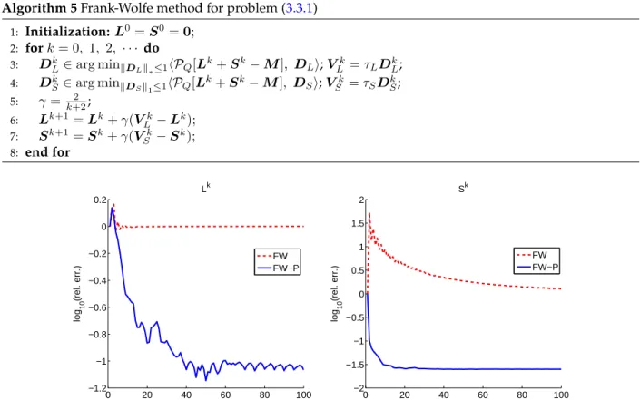
3.1 Comparisons between Algorithms 5 and 6 for problem (3.3.1) on synthetic data.. . . 50
3.2 Per-iteration cost vs. the number of frames in airport and square videos with full observation. 66 3.3 Surveillance videos.. . . 67
3.4 Face images. . . 70
4.1 Approximation errors of the first iteration.. . . 82
4.2 Approximation errors of Algorithm 11. . . 89
Rn n-dimensional real space x bold small letters as vectors
xi thei-th entry of vectorx ei thei-th standard basis
kxkp p-norm of the vectorx
kxk `2-norm of the vectorx X bold capital letters as matrices
Xi: i-th row ofXas column vector
X:j j-th column ofXas column vector
Xij the(i, j)-entry of the matrixX
kXk matrix operator norm
kXkF matrix Frobenius norm
kXk∗ matrix nuclear norm
rank(X) rank of a matrix null (X) nullspace of a matrix
⊗ outer product NK j=1R ij Ri1×i2×···×iK NK Rn R K times z }| { n×n× · · · ×n
X bold Euler script capital letters as tensors
Xi1,i2,...,iK the(i1, i2, . . . , iK)-entry of the tensorX
X(k) mode-kmatricization
X(R,C) mode-(R,C)matricization
kXkF tensor Frobenius norm
kXk tensor operator norm
δ(C) statistical dimension of convex coneC
projS[x] projection ofxonto the setS
(·)> transposition without conjugation
(·)∗ conjugate transposition, equivalent to(·)>for real vectors/matrices [k] the integer set{1, . . . , k}
X ∼ L random variableX distributed by the lawL N(0,In) standard Gaussian distribution inRn
Ber(θ) standard Bernoulli distribution with parameterθ
X ∼i.i.d.L elements in (vector- or matrix-valued)Xindependent, identically distributed by the lawL
w.h.p. short for “with high probability”
i.i.d. short for “independent, identically distributed” w.l.o.g. short for “without loss of generality”
w.r.t. short for “with respect to”
I would like to give my foremost thanks to my advisor, Professor Donald Goldfarb. It is truly a wonderful experience working with him. His great sense of humor, enthusiasm in research and inspirational words of wisdom have not only made my PhD journey exceptionally enriching and enjoyable, but will also be my most valuable life assets.
I am especially grateful to my co-advisor, Professor John Wright, who sheds the light to me on the exciting and possible interaction between fundamental theoretical progress and practical impact. His high intellectual standard, intrepid attitudes towards research difficulties and thoughtful care over the students set me a perfect role model for being a researcher, an educator and a responsible person.
I would also express special thanks to my collaborator, Professor Daniel Hsu, who also taught me the class Advanced Machine Learning. His expertise in the area of tensor and great patience on working out details have substantially helped with the thesis preparation.
I would like to give my sincere gratitude to my other dissertation committee members, Professor Garud Iyengar and Professor Daniel Bienstock. I have been greatly influenced by their courses: Convex Optimization by Garud and Integer Programming by Dan. These are the very first optimization courses that inspired my interests in the field, and set me foundations for research thereafter.
I am fortunate to have had great colleagues and friends throughout my Columbian years. During the past six years at Columbia, I have met so many good friends, which become my integral part of life. They have made my life more colorful and the office always feel like home. I have enjoyed close-knit friendship with my fellow Columbia friends: Chen Chen, Ningyuan Chen, Xingyun Chen, Yupeng Chen, Zhengyu Chen, Antoine Desir, Jing Dong, Itai Feigebaum, Jing Guo, Wenqi Hu, Bo Huang, Jingfei Jia, Henry Kuo, Yenson Lau, Anran Li, Fengpei Li, Juan Li, Xin Li, Zhige Li, Yan Liu, Zhipeng Liu, Yin Brian Lu, Carlos Lopez, Wei Liu, Zhe Liu, Lijian Lu, Ni Ma, Shiqian Ma, Gonzalo Munoz, Yanan Pei, Zhiwei Tony Qin, Qing Qu, Ju Sun, Yunjie Sun, Chun Wang, Xinshang Wang, Zheng Wang, Ji Wen, Zaiwen Wen, Linan Yang, Shuoguang Yang, Chun Ye, Wotao Yin, Chaoxu Zhou, Fan Zhang, Xiaopei Zhang, Yuqian Zhang, ...
Last but not least, my heartfelt gratitude goes to my family, particularly my parents, Weimin Mu and Xiuli Xu, and my wife, Hao Cher Han. Their unconditional love, trust and support always grant me the courage to
Apr 21, 2017 New York
Chapter 1
Introduction
Multidimensional arrays, a.k.a. tensors, generalize vectors (i.e. one-dimensional arrays) and matrices (i.e. two-dimensional arrays). They arise naturally as a flexible and integral approach to data representation and modelling, especially in problems where the underlying objects are multi-dimensional with entries indexed by several continuous and discrete variables. For instance, in collaborative filtering [KABO10] and demand forecasting [LX10,HQB15], historical ratings and sales data are often organized with indices in user ID, product ID and contextual variables including time, location and so on; in computer vision and graphics [LMWY09], visual data are naturally indexed by the specifications in space, frequency channel, time point, etc.; in statistics, higher order moments and cumulants for multivariate distributions are tensors with equal length indexed by the variables along each dimension [McC87]. Across ubiquitous tensor applications over different areas, there are two recurring challenges in general. The first one, known astensor recovery, is to recover the underlying tensor from incomplete information. For example, the ultimate goal of collaborative filtering is to figure out the missing ratings from the sparsely observed ones and thus make more precise and personalized recommendations to customers. The second challenge is on how to extract useful information from these multidimensional data, which normally relies on varioustensor decompositionsto provide a concise representation of the original tensor and moreover to capture the salient features of the underlying data.
Both challenges, tensor recoveryandtensor decomposition, are respectively addressed in this thesis. In specific, Chapter2and Chapter3, based on our previous works [MHWG14] and [MZWG16], focus on tensor recovery from both theoretical and algorithmic aspects, and Chapter4, based on our previous work [MHG15], discusses topics in tensor decomposition. In the remaining part of this chapter, the nomenclature used in the thesis will be established following an overview of each chapter.
1.1
Overview
In Chapter2, we focus on recovering low-rank tensors from incomplete information, which is a recurring problem in signal processing and machine learning. The most popular convex relaxation of this problem minimizes thesum of the nuclear norms (SNN)of the unfolding matrices of the tensor. We show that this approach can besubstantially suboptimal: reliably recovering aK-wayn×n×· · · ×ntensor of Tucker rank
(r, r, . . . , r)from Gaussian measurements requiresΩ(rnK−1)observations. In contrast, a certain (intractable) nonconvex formulation needs onlyO(rK+nrK)observations. We introduce asimple and new convex relaxation, which partially bridges this gap. Our new formulation succeeds withO(rbK/2cndK/2e)observations. The lower boundfor the SNN model follows from our new result onrecovering signals with multiple structures(e.g. sparse, low rank), which indicates the significant suboptimality of the common approach ofminimizing the sum of individual sparsity inducing norms(e.g.`1, nuclear norm). Our new tractable formulation for low-rank tensor recovery shows how the sample complexity can be reduced by designing convex regularizers that exploit several structures jointly.
Chapter3is more about an algorithmic exploration. We first build up the connection between the robust low-rank tensor recovery problem and the robust low-rank matrix recovery problem, and then focus on developing scalable optimization methods to solve the latter problem. Recovering matrices from compressive and grossly corrupted observations is a fundamental problem in robust statistics, with rich applications in computer vision and machine learning. In theory, under certain conditions, this problem can be solved in polynomial time via a natural convex relaxation, known asCompressive Principal Component Pursuit (CPCP). However, many existing provably convergent algorithms for CPCP suffer fromsuperlinear per-iteration cost, which severely limits their applicability to large-scale problems. In this chapter, we propose provably convergent, scalable and practical methods to solve CPCP withlinear per-iteration cost. Our method combines classical ideas fromFrank-Wolfeandproximal methods. In each iteration, we exploit Frank-Wolfe toupdate the low-rank component with rank-one SVDandexploit a proximal gradient step for the sparse term. Convergence results and implementation details are discussed. We also demonstrate the practicability and scalability of our approach with numerical experiments on visual data.
In Chapter4, we study a particular tensor decomposition with a wide range of applications in signal processing, machine learning and statistics. In specific, many idealized problems in higher-order statistical estimation [McC87], independent component analysis [Com94,CJ10] and parameter estimation for latent variable models [AGH+14] can be reduced to the problem of finding the symmetric canonical decomposition
of an underlyingsymmetric and orthogonally decomposable (SOD)tensor. Drawing inspiration from the matrix case, thesuccessive rank-one approximations (SROA)scheme has been proposed and shown to yield this tensor decomposition exactly, and a plethora of numerical methods have thus been developed for the tensor rank-one approximation problem. In practice, however, the inevitable errors—e.g., from estimation, computation, and modeling, necessitate that the input tensor can only be assumed to be a nearly SOD tensor—i.e., a symmetric tensor slightly perturbed from the underlying SOD tensor. Chapter4proves that even in the presence of perturbation, SROA can still robustly recover the symmetric canonical decomposition of the underlying tensor. It is shown that when the perturbation error is small enough, the approximation errors do not accumulate with the iteration number. Numerical results are presented to support the theoretical findings.
1.2
Notations and Preliminaries
The notations, used throughout the thesis, are largely borrowed from [Kie00,Lim05,KB09].
Theorderof a tensor is referred to as the number of dimensions, also known asmodesorways. Some trivial examples of tensors are scalars, vectors and matrices.Scalars(tensors of order zero) are denoted by lowercase letters, e.g.,x. Vectors(tensors of order one) are denoted by boldface lowercase letters, e.g.,x. Matrices (tensor of order two) are denoted by boldface capital letters, e.g.,X.High-order tensors(order three or higher) are denoted by boldface Euler script letters, e.g.,X.
For a tensorX of orderK, its(i1, i2, . . . , iK)-th entry is denoted asXi1,i2,...,iK. Thei-th entry of a vector xis denoted asxi, the(i, j)-th entry of a matrixXis denoted asXij.
Afiberof a tensorX is a column vector defined by fixing each index ofX except one. Thei-th column of a matrixX, denoted byX:i, is a mode-1fiber, and thei-th row ofX, denoted byXi:, is a mode-2fiber, where a colon adapted from many numerical computing languages, e.g. Matlab, is commonly used to indicate all elements of one particular mode. Third-order tensors havecolumn, row and tube fibers, respectively, denoted asX:jk,Xi:kandXij:, which by convention are all considered as column vectors when extracted fromX.
A sliceof a tensorX is a two-dimensional section defined by fixing all indices except two ones. A third-order tensor hashorizontal, lateral and frontal slices, respectively, denoted asXi::,X:j:andX::k.
The set ofK-wayI1×I2× · · · ×IKtensor,RI1×I2×···×IK
, in short, is denoted byNKj=1R Ij
. For any tensors
X,Y ∈NKj=1R Ij
, their inner product is defined as the sum of all the element-wise products, i.e.
hX,Yi:= I1 X i1=1 I2 X i2=1 · · · IK X iK=1 Xi1i2···iKYi1i2···iK. (1.2.1)
Tensor as multilinear map. In addition to being considered as a multi-way array, a tensorX ∈NKj=1R Ij
can also be interpreted as amultilinear mapin the following sense: for any matricesVi∈RIi×mi
fori∈[K], we interpretX(V1,V2, . . . ,VK)as a tensor inRm1×m2×···×mp whose(i1, i2, . . . , iK)-th entry is X(V1,V2, . . . ,Vp) i1,i2,...,iK := X ji∈[I1] X j2∈[I2] · · · X jK∈[IK] Xj1,j2,...,jp(V1)j1i1(V2)j2i2· · ·(VK)jKiK. (1.2.2)
This multilinear interpretation is a powerful tool to conceptually simplify and visualize the notion of tensor, and will be frequently exploited throughout the thesis.
Example 1.1 To better understand this interpretation, we provide several examples below.
. K= 2(namely,X is a matrix of sizen1byn2):
X(V1,V2) =V1>XV2∈Rm1×m2. (1.2.3)
. Each entry of the tensor can also be expressed as the scalar returned by applying the multilinear map
defined by the tensor on standard basis vectors correspondingly. In specific, for anyi1 ∈ [I1], i2 ∈
[I2], . . . , andiK ∈[IK],
X(ei1,ei2, . . . ,eiK) =Xi1,i2,...,iK, (1.2.4)
whereeidenotes thei-th standard basis.
. i1=i2=· · ·=iK =nandVi=x∈Rnfor alli∈[K]:
Xx⊗K :=X(x,x, . . . ,x | {z } K times ) = X i1,i2,...,iK∈[n] Xi1,i2,...,iKxi1xi2· · ·xiK, (1.2.5)
which defines a homogeneous polynomial of degreeK.
Tensor norms. Two tensor norms will be frequently visited in this thesis. For a tensorX ∈NKj=1R Ij
, its Frobenius normis defined as
kXkF :=phX,Xi= v u u t I1 X i1=1 I2 X i2=1 · · · IK X iK=1 X2 i1i2···iK; (1.2.6)
and itsoperator normis defined as
kXk:= max
Matricization. Matricization, also known asunfoldingorflattening, is the procedure of rearranging the elements from a tensor into a matrix. This can be a useful trick to simplify the problem from the tensor domain to the matrix one, which might be well studied in the literature. Admittedly, there are tons of ways to put the elements of a multi-way array into a matrix. We are particularly interested in matricizations that can preserve certain algebraic structures of the original tensor. Several ones most relevant to the thesis are described below.
Themode-kmatricizationof a tensorX ∈Ni∈[K]RIiyields a matrix denoted byX(k)∈RIk×Πi6=kIi, whose columns are the mode-kfibers arranged via certain lexicographical order of the indices except for thek-th index. More rigorously, the(i1, i2, . . . , iK)-th element ofXis mapped to the(in, j)-th element inX(k), where
j = 1 + X k6=l∈[K] il−1 · Y n6=l0∈[l−1] Il0 . (1.2.8)
There are also multiple ways we can stack the tensor into a vector. In this thesis, we specifically define
vec(X) :=vec X(1)
. (1.2.9)
Example 1.2 Consider a 3-way tensorX ∈R3×4×2, whose frontal slices are
X::1= 1 4 7 10 2 5 8 11 3 6 9 12 and X::2= 13 16 19 22 14 17 20 23 15 18 21 24 . (1.2.10)
Then we can matricizeX along the first, the second and the third modes respectively, which yields
X(1) = 1 4 7 10 13 16 19 22 2 5 8 11 14 17 20 23 3 6 9 12 15 18 21 24 , (1.2.11) X(2)= 1 2 3 13 14 15 4 5 6 16 17 18 7 8 9 19 20 21 10 11 12 22 23 24 , (1.2.12)
X(3)= 1 2 3 4 · · · 10 11 12 13 14 15 16 · · · 22 23 24 . (1.2.13)
Vectorization will yield a column vector inR24:
vec(X) = vec(X(1)) =
1 2 3 4 · · · 21 22 23 24
>
. (1.2.14)
The mode-kmatricization can be considered as we partition the set of modes[K] ={1,2,· · · , K}into
{k}and[K]/{k}. Once thinking about mode-kmatricization in this direction, it is natural to enrich the class
of matricization by considering more general partitions over the set[K].
Let the ordered setsR={r1, r2, . . . , rL}andC={c1, c2, . . . , cM}be a partitioning of[K] ={1,2, . . . , K}. The matricized tensor induced by this partition{R,C}is a matrix denoted byX(R×C)∈RJ×Kwhere
J = Y k∈R Ik, K= Y k∈C Ik, and
the(i1, i2, . . . , iK)-th element ofX is mapped to the(i, j)-th entry in this mode-(R,C)matricizationXR×C with i= 1 + X l∈[L] irL−1 · Y l0∈[l−1] Irl0 , (1.2.15) j= 1 + X m∈[M] irm−1 · Y m0∈[m−1] Irm0 . (1.2.16)
Remark 1.3 For the mode-kmatricizationX(k), we can regard it as the matricized tensor induced byR={k} andC={1,2, . . . , k−1, k+ 1, . . . , K}, i.e.
X(k)=X({k}×{1,2,...,k−1,k+1,...,K}). (1.2.17)
For the vectorizationvec(X), conventionally, we can define it as the matricized tensor induced byR= [K]and
C=∅, i.e. vec(X) =X([K]×∅).
This more general treatment of matricization is first formally introduced by Kolda [Kol06]. The concept might not be much useful and appreciated for tensors of order three. In contrast, it will provide substantially more freedom in the choice of tensor flattening once the fourth dimension and beyond come on the stage, and is frequently revisited recently in different contexts including the low-rank tensor recovery [MHWG14,
JMZ15], and the semidefinite programming approach to relax the best tensor rank-one approximation [JMZ14,NW14,HJLW16].
Example 1.4 Consider a four-way tensorX ∈R2×2×2×2with elements specified as
X::11= 1 3 2 4 , X::21= 5 7 6 8 , X::12= 9 11 10 12 , X::22= 13 15 14 16 . (1.2.18)
All the mode-kunfoldings will yield a matrix inR2×8, e.g.,
X(1)= 1 3 5 7 9 11 13 15 2 4 6 8 10 12 14 16 . (1.2.19)
However, the matricized tensor induced byR={1,2}andC={3,4}yields more balanced square matrix:
X({1,2}×{3,4})= 1 5 9 13 2 6 10 14 3 7 11 15 4 8 12 16 ∈R4×4. (1.2.20)
A sharp observation may lead to the following property that
X({1,2}×{3,4})=reshape(X(1),4,4).
It turns out the above equality holds more universally in tensor unfolding.
Matlab implementations for matricization. The folding and unfolding procedures discussed above can be implemented in surprisingly simple Matlab instructions. The code below is adapted from Kolda [Kol06].
1 size = [2,2,2,2];
2 X = reshape(1:16, size); % the four−way tensor in Example 1.4 3
4 % mode−1 matricization 5 R = [1]; C = [2,3,4];
6 J = prod(size(R)); K = prod(size(C));
7 Y = reshape(permute(X,[R,C]), J,K); % mode−1 unfolding
9
10 % mode−{R,C} matricization 11 R = [1,2]; C = [3,4];
12 J = prod(size(R)); K = prod(size(C));
13 Y = reshape(permute(X,[R,C]), J,K); % matricized tensor induced by R and C
14 Z = ipermute(reshape(Y,[size(R), size(C)]), [R C]); % convert back to the original tensor
Tensor-Matrix Multiplication. Themode-kmatrix productbetween a tensorX ∈RI1×I2×···×IK
and a matrix U ∈RJ×Ik
, denoted byX×kU, returns a new tensor of sizeI1×I2× · · · ×Ik−1×J×Ik+1×Ik+2× · · · ×IN, with elements specified as
(X ×kU)i1···ik−1jik+1···iK:=
X
in∈Ik
Xi1i2···iKUjin. (1.2.21)
Two equivalent definitions, using mulilinear map and mode-kmatricization, are also available and may provide more insights into this tensor-matrix multiplication.
First, it can be verified by checking definition that
X ×kU =X I, · · ·,I | {z } k−1times , U> , I,· · · , I | {z } n−k times . (1.2.22)
Moreover, thek-mode matrix product can be considered as each mode-kfiber is multiplied by the matrix U, which can be precisely expressed as
Y =X ×kU ⇐⇒ Y(k)=UX(k). (1.2.23)
Example 1.5 Consider the product along the first mode between the tensorX in Example(1.2)and U = 1 3 5 2 4 6 . (1.2.24)
Then the frontal slices ofY =X ×1U ∈R2×4×2are
Y::1=UX::1= 22 49 76 103 28 64 100 136 and Y::2=UX::2= 130 157 184 211 172 208 244 280 . (1.2.25)
discussions in later chapters: X ×mA×nB= X ×nB×mA if m6=n X ×n(BA) if m=n. (1.2.26)
Literally,×kis commutative when they are applied on different modes. But when they are applied on the same mode,×kis no longer commutative as matrix multiplication is not commutative.
Rank-one tensors. Thevector outer productis denoted by the symbol⊗. The outer product ofKvectors,
{vi}i∈[K]∈
×
K k=1R Ik is defined as (v1⊗v2⊗ · · · ⊗vK)i1i2···iK := (v1)i1(v2)i2· · ·(vK)iK ∀ik∈[Ik] and k∈[K]. (1.2.27)This means that each element of the tensor is the product of vector elements at the corresponding entries. The definition (1.2.27) also extrapolates the concept of rank-one matrix to rank-one tensor. AK-way tensorX ∈ RI1×I2×···×INis rank one if there exists{vi}i∈[K]∈
×
K k=1R
Ik
such thatXcan be expressed asv1⊗v2⊗· · ·⊗vK. Rank-one tensors play fundamental roles in tensor decomposition where different ways to express the tensor into the sum of rank-one tensors are pursued.
Symmetric tensors. A tensor is calledcubicalif it has the same size along each mode. The set of real order-K cubical tensors with dimensionnalong each mode is denoted byNKRn. A cubical tensorX ∈NKRnis calledsymmetricif its entries are invariant under any permutation of their indices: for anyi1, i2, . . . , iK∈[n] :
Xi1i2...iK=Xiπ(1)iπ(2)...iπ(K) (1.2.28)
for any permutation mappingπon[K]. This definition naturally extends the concept of symmetry from matrices to tensors of higher order, and will be the mathematical object of our main focus in Chapter4.
A three-way tensorX ∈Rn×n×n, for example, is symmetric if
Xijk=Xikj=Xjik=Xjki =Xkij=Xkji, ∀ i, j, k∈[n]. (1.2.29)
A tensorX ∈NKRnisdiagonalifXi1i2···iKis zero unlessi1 =i2=· · ·=iK. Literally speaking, this
describes a tensor with nonzero elements possible only on the superdiagonal entries, which is a higher order analogue of diagonal matrices. Clearly, a diagonal tensor is symmetric.
Then rank-one tensor v⊗K:=v⊗v⊗ · · · ⊗v | {z } K times ∈ K O Rn
is another commonly encountered example of symmetric tensors. The converse is also true that a symmetric tensorX of rank-one can always be written asX =v⊗K.
When the tensorX ∈NKRnis symmetric, its operator norm originally defined as
kXk = max
kxik=1 X(x1,x2, . . . ,xK) (1.2.30) can be simplified by restrictingx1=x2=· · ·=xKwithout loss of generality (see, e.g., [CHLZ12,ZLQ12]), namely kXk = max kxk=1 Xx⊗K = max x2 1+x22+···+x2n=1 X i1∈[n] X i2∈[n] · · · X iK∈[n] Xi1i2···iKxi1xi2· · ·xiK . (1.2.31)
The definition of symmetric tensors also immediately yield the following property:
vec X I,x,x,· · ·,x,x | {z } K−1times = vec X x,I,x,· · ·,x,x =· · ·= vec X x,x,x,· · · ,x,I .
In order to refer to the above quantity more conveniently, we define
Xx⊗K−1:=X(x, . . . ,x,I)∈Rn,
(1.2.32)
Xx⊗K−1i = X
i1i2...iK−1∈[n]
Xi1i2...iK−1ixi1xi2· · ·xiK−1. (1.2.33)
It can be also verified that the vectorXx⊗K−1is aligned with the gradient∇x
Xx⊗K as ∇x Xx⊗K =K·Xx⊗K−1. (1.2.34)
Tensor decompositions and ranks. TheCANDECOMP/PARAFAC (CP) decomposition[CC70,Har70] fac-torizes a tensor into a sum of rank-one tensor components. Mathematically, the CP decomposition of
X ∈RI1×I2×···×IK is given by X =Jλ;A(1),A(2), . . . ,A(K)K:= X r∈[R] λr·a(1)r ⊗a (2) r ⊗ · · · ⊗a (K) r . (1.2.35)
Hereλ = [λ1, λ2, . . . , λR]> ∈ RR+, a (k) r
= 1for all(r, k)∈ [R]×[K]andA
(k) = [a(k) 1 ,a (k) 2 ,· · ·,a (k) R ] ∈ RIk×R
for allk∈[K]. With the CP decomposition provided in (1.2.35), the tensor elementXi1,i2,...,iKcan be
concisely expressed as Xi1,i2,...,iK = X r∈[R] λr Y k∈[K] a(k)r,i k. (1.2.36)
TheCP-rankof the tensorX is aligned with concept of matrix ranks. Recall that the rank of a matrixX ∈m×n is defined as smallest number such thatX can be written as the sum of rank-one matrices. Similarly, the CP-rank of the tensorX is the smallest numberRsuch that (1.2.35) holds.
TheTucker decomposition[Tuc66] searches for the following pattern:
X =JG;A(1),A(2), . . . ,A(K)K (1.2.37) =G×1A(1)×2A(1)×3· · · ×KA(K) (1.2.38) = X r1∈[R1] · · · X rK∈[RK] Gr1r2···rKa (1) r1 ⊗a (2) r2 ⊗ · · · ⊗a (K) rK (1.2.39) Here,G∈Rr1×r2×···×rK
is calledcore tensorand the orthogonal matrixA(k)= [a(k)1 ,a (k) 2 ,· · ·,a
(k)
r ]∈RIk×r
is calledfactor matrix. TheTucker-rankofX, denoted byranktc(X), is aK-tuple, describing the rank of each mode-kunfolding matrix, i.e.
ranktc(X) := rank(X(1)),rank(X(2)), . . . ,rank(X(K))
. (1.2.40)
There are also a number of other tensor decompositions [CC70,Har72,CPK80,HL96] as variants of the above CP and Tucker ones by imposing more constraints over the factors. These decompositions are not that relevant with the thesis and thus will not be discussed in details.
Chapter 2
Low-Rank Tensor Recovery
2.1
Introduction
Tensors arise naturally in problems where the goal is to estimate a multi-dimensional object whose entries are indexed by several continuous or discrete variables. For example, a video is indexed by two spatial variables and one temporal variable; a hyperspectral datacube is indexed by two spatial variables and a frequency/wavelength variable. While tensors often reside in extremely high-dimensional data spaces, in many applications, the tensor of interest islow-rank, or approximately so [KB09], and hence has much lower-dimensional structure. The general problem of estimating a low-rank tensor has applications in many different areas, both theoretical and applied: e.g., estimating latent variable graphical models [AGH+14], classifying audio [MSS06], mining text [CC12], processing radar signals [NS10], multilinear multitask learning [RPABBP13] , to name a few.
In this chapter, we consider the problem of recovering aK-way tensorX ∈Rn1×n2×···×nKfrom linear measurementsz =G[X] ∈Rm. Typically,mN =QKi=1ni, and so the problem of recoveringX from zisill-posed. In the past few years, tremendous progress has been made in understanding how to exploit structural assumptions such as sparsity for vectors [CRT06] or low-rankness for matrices [RFP10] to develop computationally tractable methods for tackling ill-posed inverse problems. In many situations, convex optimization can estimate a structured object from near-minimal sets of observations [NRWY12,CRPW12, ALMT14]. For example, ann×nmatrix of rankrcan, with high probability, be exactly recovered fromCnr generic linear measurements, by minimizing the nuclear normkXk∗=
P
iσi(X). Since a rankrmatrix has
In contrast, the correct generalization of these results to low-rank tensors is not obvious. The numerical algebra of tensors is fraught with hardness results [HL13]. For example, even computing a tensor’s (CP) rank [CC70,Har70], rankcp(X) = min r|X =Xr i=1a (i) 1 ⊗ · · · ⊗a (i) K , (2.1.1)
is NP-hard in general. The nuclear norm of a tensor is also intractable, and so we cannot simply follow the formula that has worked for vectors and matrices.
With an eye towards numerical computation, many researchers have studied how to recover tensors of smallTucker rank[Tuc66]. The Tucker rank, also known asn-rank, of aK-way tensorX is aK-dimensional vector whosei-th entry is the (matrix) rank of the mode-iunfoldingX(i)ofX:
ranktc(X) = rank(X(1)),· · ·,rank(X(K))
. (2.1.2)
Here, the matrixX(i) ∈ Rni×
Q
j6=inj
is obtained by concatenating all the mode-ifibers ofX as column vectors. Eachmode-ifiberis anni-dimensional vector obtained by fixing every index ofX but thei-th one. The Tucker rank ofX can be computed efficiently using the (matrix) singular value decomposition. For this reason, we focus on tensors of low Tucker rank. However, we will see that our proposed regularization strategy also automatically adapts to recover tensors of low CP rank, with reduction in the required number of measurements.
The definition (2.1.2) suggests a natural, tractable convex approach to recovering low-rank tensors: seek theXthat minimizesPiλi
X(i)
∗out of allXsatisfyingG[X] =z. We will refer to this as the
sum-of-nuclear-norms (SNN)model. Originally proposed in [LMWY09], this approach has been widely studied [GRY11, SDS10,STDLS13,TSHK11] and applied to various datasets in imaging [SHKM14,KS13,LL10,LYZY10].
Perhaps surprisingly, we show that this natural approach can be substantially suboptimal. Moreover, we will suggest a simple new convex regularizer with provably better performance. Supposen1=· · ·=nK=n, andranktc(X)(r, r, . . . , r). LetTrdenote the set of all such tensors,1namely
Tr:=X ∈Rn×n×···×n| ranktc(X)(r, r, . . . , r) . (2.1.3)
We will consider the problem of estimating an elementX ofTrfrom Gaussian measurementsG(i.e.,zi=
hGi,Xi, whereGihas i.i.d. standard normal entries). To describe a generic tensor inTr, we need at most
rK+rnKparameters. In Section2.2, we show that a certain nonconvex strategy can recover allX ∈Tr
1
To keep the presentation in this chapter compact, we state most of our results regarding tensors inTr, although it is not difficult to modify them for general tensors.
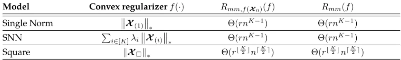
exactly whenm >(2r)K+ 2nrK. In contrast, the best known theoretical guarantee for SNN minimization, due to Tomioka et al. [TSHK11], shows thatX ∈Trcan be recovered (or accurately estimated) from Gaussian measurementsG, providedm= Ω(rnK−1). In Section2.3, we prove that this number of measurements is alsonecessary: accurate recovery is unlikely unlessm= Ω(rnK−1). Thus, there is a substantial gap between an ideal nonconvex approach and the best known tractable surrogate. In Section2.4, we introduce a simple alternative, which we call thesquare reshapingmodel, which reduces the required number of measurements toO(rbK/2cndK/2e). ForK >3, we obtain an improvement of a multiplicative factor polynomial inn.
Our theoretical results pertain to Gaussian operatorsG. The motivation for studying Gaussian mea-surements is threefold. First, Gaussian meamea-surements may be of interest for compressed sensing recovery [Don06], either directly as a measurement strategy, or indirectly due to universality phenomena [BLM12]. Moreover, the available theoretical tools for Gaussian measurements are very sharp, allowing us to rigorously investigate the efficacy of various regularization schemes, and prove both upper and lower bounds on the number of observations required. Furthermore, the results with respect to Gaussian measurements have direct implications to the minimax risk for denoising [OH16,ALMT14]. In Section2.4, we demonstrate that our qualitative conclusions carry over to more realistic measurement models, such as random subsampling [LMWY09]. We expect our results to be of great interest for a wide range of problems in tensor completion [LMWY09], robust tensor recovery/decomposition [LYZY10,GQ14] and sensing.
Our technical approach draws on, and enriches, the literature on general structured model recovery. The surprisingly poor behavior of the SNN model is an example of a phenomenon first discovered by Oymak et al. [OJF+12]: for recovering objects with multiple structures, a combination of structure-inducing norms is often not significantly more powerful than the best individual structure-inducing norm. Our lower bound for the SNN model follows from a general result of this nature, which we prove using the novel geometric framework of [ALMT14]. Compared to [OJF+12], our result pertains to a more general family of regularizers, and gives sharper constants. In addition, for low-rank tensor recovery problem, we demonstrate the possibility to reduce the number of generic measurements through a new convex regularizer that exploits several sparse structures jointly.
2.2
Bounds for Non-Convex Recovery
In this section, we introduce a non-convex model for tensor recovery, and show that it recovers low-rank tensors from near-minimal numbers of measurements. While our nonconvex formulation is computationally
intractable, it gives a baseline for evaluating tractable (convex) approaches.
For a tensor of low Tucker rank, the matrix unfolding along each mode is low-rank. Suppose we observe
G[X0]∈Rm. We would like to attempt to recoverX0by minimizing some combination of the ranks of the unfoldings, over all tensorsX that are consistent with our observations. This suggests avector optimization problem [BV04, Chap. 4.7]:
minimize(w.r.t.RK
+) ranktc(X) subject to G[X] =G[X0]. (2.2.1)
In vector optimization, a feasible point is calledPareto optimalif no other feasible point dominates it in every criterion. In a similar vein, we say that (2.2.1) recoversX0if there does not exist any other tensorX that is consistent with the observations and has no larger rank along each mode:
Definition 2.1 We callX0recoverable by(2.2.1)if the set
{X06=X0| G[X0] =G[X0], ranktc(X0)RK
+ ranktc(X0)}=∅.
This is equivalent to saying thatX0is the unique optimal solution to thescalaroptimization: minimizeX max i rank(X (i)) rank(X0(i)) subject to G[X] =G[X0]. (2.2.2)
The problems (2.2.1)-(2.2.2) are not tractable. However, they do serve as a baseline for understanding how many generic measurements are required to recoverX0from an information theoretic perspective.
The recovery performance of program (2.2.1) depends heavily on the properties ofG. Suppose (2.2.1) fails to recoverX0∈Tr. Then there exists anotherX0∈Trsuch thatG[X0] =G[X0]. So, to guarantee that (2.2.1) recoversanyX0∈Tr, a necessary and sufficient condition is thatGis injective onTr, which can be implied by the conditionnull(G)∩T2r={0}. Consequently, ifnull(G)∩T2r={0}, (2.2.1) will recover anyX0∈Tr. We expect this to occur when the number of measurements significantly exceeds the number of intrinsic degrees of freedom of a generic element ofTr, which isO(rK+nrK). The following theorem shows that whenmis approximately twice this number, with probability one,Gis injective onTr:
Theorem 2.2 Wheneverm≥(2r)K+ 2nrK+ 1, with probability one,null(G)∩T2r={0}, and hence(2.2.1) recovers everyX0∈Tr.
The proof of Theorem2.2follows from a covering argument, which we establish in several steps. Let
The following lemma shows that the required number of measurements can be bounded in terms of the exponent of the covering number forS2r, which can be considered as a proxy for dimensionality:
Lemma 2.3 Suppose that the covering number forS2rwith respect to Frobenius norm, satisfies
N(S2r,k·kF, ε) ≤ (β/ε) d
, (2.2.4)
for some integerdand scalarβthat does not depend onε. Then ifm≥d+1, with probability onenull (G)∩S2r=∅, which implies thatnull (G)∩T2r={0}.
It just remains to find the covering number ofS2r. We use the following lemma, which uses the triangle inequality to control the effect of perturbations in the factors of the Tucker decomposition
[[C;U1,U2,· · ·,UK]] :=C×1U1×2U2×3· · · ×KUK, (2.2.5)
where themode-i(matrix) productof tensorAwith matrixBof compatible size, denoted asA×iB, outputs a tensorCsuch thatC(i)=BA(i).
Lemma 2.4 LetC,C0∈Rr1,...,rK, andU
1,U10 ∈Rn1×r1, . . . ,UK,UK0 ∈R nK×rKwithU∗ iUi=Ui0 ∗ Ui0 =I, andkCkF =C0 F = 1. Then [[C;U1, . . . ,UK]]−[[C0;U10, . . . ,UK0 ]] F ≤ C−C0 F+ K X i=1 kUi−Ui0k. (2.2.6)
Using this result, we construct anε-net forS2rby buildingε/(K+ 1)-nets for each of theK+ 1factorsC and{Ui}. The total size of the resultingεnet is thus bounded by the following lemma:
Lemma 2.5 N(S2r,k·kF, ε) ≤ (3(K+ 1)/ε)
(2r)K+2nrK
With these observations in hand, Theorem2.2follows immediately.
2.3
Convexification: Sum of Nuclear Norms?
Since the nonconvex problem (2.2.1) is NP-hard for generalG, it is tempting to seek a convex surrogate. In matrix recovery problems, the nuclear norm is often an excellent convex surrogate for the rank [Faz02,RFP10, Gro11]. It seems natural, then, to replace the ranks in (2.2.1) with nuclear norms. Due to convexity, the
resulting vector optimization problem can be solved by the following scalar optimization: min X K X i=1 λikX(i)k∗ s.t. G[X] =G[X0], (2.3.1)
whereλ≥0. The optimization (2.3.1) was first introduced by [LMWY09] and has been used successfully in applications in imaging [SHKM14,KS13,LL10,EAHK13,LYZY10]. Similar convex relaxations have been considered in a number of theoretical and algorithmic works [GRY11,SDS10,TSHK11,STDLS13]. It is not too surprising, then, that (2.3.1) provably recovers the underlying tensorX0, when the number of measurements
mis sufficiently large. The following is a (simplified) corollary of results of Tomioka et. al. [TSHK11]2
: Corollary 2.6 (of [TSHK11], Theorem 3) Suppose thatX0has Tucker rank(r, . . . , r), andm≥CrnK−1, whereCis a constant. Then with high probability,X0is the optimal solution to(2.3.1), with eachλi= 1.
This result shows that thereisa range in which (2.3.1) succeeds: loosely, when we undersample by at most a factor ofm/N ∼r/n. However, the number of observationsm∼rnK−1is significantly larger than the number of degrees of freedom inX0, which is on the order ofrK+nrK. Is it possible to prove a better bound for this model? Unfortunately, we show that in generalO(rnK−1)measurements are alsonecessaryfor reliable recovery using (2.3.1):
Theorem 2.7 LetX0∈Trbe nonzero. Setκ= mini
n (X0)(i) 2 ∗/kX0k 2 F o
×nK−1. Then if the number of
measurementsm≤κ−2,X0is not the unique solution to(2.3.1), with probability at least1−4 exp(−(κ−m−2)
2
16(κ−2) ). Moreover, there existsX0∈Trfor whichκ=rnK−1.
This implies that Corollary2.6(as well as some other results of [TSHK11]) is essentially tight. Unfortunately, it has negative implications for the efficacy of the SNN model in (2.3.1): although a generic elementX0ofTr can be described using at mostrK+nrKreal numbers, we requireΩ(rnK−1)observations to recover it using (2.3.1). Theorem2.7is a direct consequence of a much more general principle underlying multi-structured recovery, which is elaborated next. After that, in Section2.4, we show that for low-rank tensor recovery, better convexifying schemes are available.
2.3.1
General lower bound for multiple structures
The poor behavior of (2.3.1) is an instance of a much more general phenomenon, first discovered by Oymak et. al. [OJF+12]. Our target tensorX0hasmultiplelow-dimensional structures simultaneously: it is low-rank
2Tomioka et. al. also show noise stability whenm= Ω(rnK−1)and give extensions to the case where theranktc(X0) = (r1, . . . , r
K) differs from mode to mode.
alongeachof theK modes. In practical applications, many other suchsimultaneously structuredobjects could also be of interest. For sparse phase retrieval problems in signal processing [OJF+12], the task can be rephrased to infer a block sparse matrix, which implies both sparse and low-rank structures. In robust metric learning [LML13], the goal is to estimate a matrix that is column sparse and low rank concurrently. In computer vision, many signals of interest are both low-rank and sparse in an appropriate basis [LRZM12]. To recover such simultaneously structured objects, it is tempting to build a convex relaxation by combining the convex relaxations for each of the individual structures. In the tensor case, this yields (2.3.1). Surprisingly, this combination is often not significantly more powerful than the best single regularizer [OJF+12]. We obtain Theorem2.7as a consquence of a new, general result of this nature, using a geometric framework introduced in [ALMT14]. Compared to [OJF+12], this approach has a clearer geometric intuition, covers a more general class of regularizers3and yields sharper bounds.
Setup. In general, we are interested in recovering a signalx0with several low-dimensional structures simultaneously, based on generic measurements with respect tox0. Here the target signalx0could lie in any finite dimensional Hilbert space (e.g. a vector inRn, a matrix inRn1×n2
, a tensor inRn1×n2×···×nK
), but without loss of generality, we will considerx0∈Rn. Letk·k(i)be the penalty norm corresponding to thei-th structure (e.g.`1, nuclear norm). Consider the followingsum-of-norms (SoN)model,
min
x∈Rn
f(x) :=λ1kxk(1)+λ2kxk(2)+· · ·+λKkxk(K) subject to G[x] =G[x0], (2.3.2)
whereG[·]is a Gaussian measurement operator, andλ>0. In the subsequent analysis, we will evaluate the performance of (2.3.2) in terms of recoveringx0, where the only assumption we require is:
Assumption 2.8 The target signalx0is nonzero.
Optimality condition. Isx0the unique optimal solution to (2.3.2)? Recall that the descent cone of a function
f at a pointx0is defined as
C(f,x0) := cone{v|f(x0+v)≤f(x0)}, (2.3.3)
which, in short, will be denoted asC. Thenx0is the unique optimal solution if and only if
null(G)∩ C={0}. (2.3.4)
Conversely, recovery fails ifnull(G)has nontrivial intersection withC.
3
SinceGis a Gaussian operator,null(G)is a uniformly oriented random subspace of dimension(n−m). This random subspace is more likely to have nontrivial intersection withCifCislarge, in a sense we will make precise.
Denote the polar cone ofCasC◦, i.e.
C◦:= u∈Rn| sup x∈C hu,xi ≤0 . (2.3.5)
Because polarity reverses inclusion, we expect thatCwill belargewheneverC◦issmall, which leads us to control the size ofC◦.
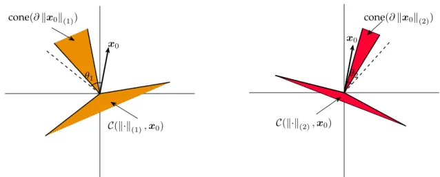
cone(∂kx0k(1)) x0 θ1 C(k·k(1),x0) cone(∂kx0k(2)) x0 θ2 C(k·k(2),x0)
Figure 2.1: Cones and their polars for convex regularizersk·k(1)andk·k(2) respectively. Suppose ourx0 has two sparse structures simultaneously. Regularizerk·k(1)has a larger conic hull of subdifferential atx0, i.e. cone(∂kx0k(1)), which results in a smaller descent cone. Thus minimizingk·k(1)is more likely to recoverx0than minimizingk·k(2). Consider convex regularizerf(x) =kx0k(1)+kx0k(2). Suppose as depicted,θ1≥θ2. Then both cone(∂kx0k(1))and cone(∂kx0k(2))are in the circular cone circ(x0, θ1). Thus we have: cone ∂f(x0)
= cone(∂kx0k(1)+∂kx0k(2)) ⊆ convcirc(x0, θ1),circ(x0, θ2) =circ(x0, θ1).
Asf(x0)6= 0 = minx∈Rnf(x), it can be verified that [Roc97, Thm. 23.7]
C◦= cone (∂f(x0)) = cone X i∈[K] λi∂fi(x0) , (2.3.6)
where the sum is made in Minkowski sense.
In order to control the size ofCobased on (2.3.6), we will next establish some basic geometric properties for each single norm.
Properties for each single norm. Consider a general single normk·k and denote its dual norm (a.k.a. polar function) ask·k◦, i.e. for anyu∈Rn,
kuk◦:= sup
kxk≤1
hx,ui. (2.3.7)
DefineL:= supx6=0 kxk/kxk, which implies thatk·kisL-Lipschitz:kxk≤Lkxkfor allx. Then we also havekuk ≤Lkuk◦for alluas
kuk◦ = sup kxk≤1 hx,ui ≥ sup Lkxk≤1 hx,ui= sup kxk≤1/L hx,ui= 1 Lkuk. (2.3.8)
In addition, noting that
∂k·k(x) =u| hu,xi=kxk, kuk◦≤1 , (2.3.9)
for anyu∈∂k·k(x0), we have
cos (∠(u,x0)) := hu,x0i kuk kx0k ≥ kx0k Lkuk◦kx0k ≥ kx0k Lkx0k . (2.3.10)
A more geometric way of summarizing this fact is as follows: forx6=0, let
circ(x, θ) ={z|∠(z,x)≤θ}, (2.3.11)
denote thecircular conewith axisxand angleθ. Then withθ:= cos−1(kx0k/Lkx0k),
∂k·k(x0)⊆circ (x0, θ). (2.3.12)
Table2.1describes the angle parametersθfor various structure inducing norms. Notice that in general, more complicatedx0leads to smaller anglesθ. For example, ifx0is ak-sparse vectors with entries all of the same magnitude, andk·kthe`1norm,cos2θ=k/n. Asx0becomes more dense,∂k·kis contained in smaller and smaller circular cones.
Polar cone⊆circular cone. Forf =Piλik·k(i), notice that every element of∂f(x0)is a conic combination of elements of the∂k·k(i)(x0). Since each of the∂k·k(i)(x0)is contained in a circular cone with axisx0,
Lemma 2.9 Forx06=0, setθi= cos−1
kx0k(i)/Likx0k
, whereLi= supx6=0 kxk(i)/kxk. Then
C◦= cone (∂f(x0))⊆circ x0,max i∈[K]θi . (2.3.13)
So, the subdifferential of our combined regularizerfis contained in a circular cone whose angle is given by the largest of theθi. Figure2.1visualizes this geometry.
Statistical Dimension. How does this behavior affect the recoverability ofx0via (2.3.2)? The informal reasoning above suggests that asθbecomes smaller, the descent coneCbecomes larger, and we require more measurements to recoverx0. This can be made precise using the elegant framework introduced by Amelunxen et al. [ALMT14]. They define thestatistical dimensionof the convex coneCto be the expected norm square of the projection of a standard Gaussian vector ontoC:
δ(C) :=Eg∼i.i.d.N(0,1)
h
kPC(g)k2
i
(2.3.14)
Using tools from spherical integral geometry, Amelunxen et al. [ALMT14] show that for linear inverse problems with Gaussian measurements, a sharp phase transition in recoverability occurs aroundm=δ(C). Since we attempt to derive a necessary condition for the success of (2.3.2), we need only one side of their result with slight modifications:
Corollary 2.10 LetG:Rn→Rmbe a Gaussian operator, andCa convex cone. Then ifm≤δ(C), P[C ∩null(G) ={0}] ≤ 4 exp −(δ(C)−m) 2 16δ(C) . (2.3.15)
Table 2.1: Concise models and their surrogates.For each normk·k, the third column describes the range of achievable angles
θ. Largercosθcorresponds to a smallerCo, a largerC, and hence a larger number of measurements required for reliable recovery.
Object Complexity Measure Relaxation cos2θ κ=ncos2θ
Sparsex∈Rn k=kxk0 kxk1 [ 1 n, k n] [1, k] Column-sparsex∈Rn1×n2 c= #{j|xe j6=0} Pjkxejk [n12,nc2] [n1, cn1] Low-rankx∈Rn1×n2 (n1≥n2) r= rank(x) kxk∗ [n1 2, r n2] [n1, rn1]
To apply this result to our problem, we need to have a lower bound on the statistical dimensionδ(C), of the descent coneCoff atx0. Using the Pythagorean theorem, monotonicity ofδ(·), and Lemma2.9, we calculate
δ(C) = n−δ(C◦) = n−δ(cone(∂f(x
0))) ≥ n−δ(circ(x0,max
i θi)). (2.3.16) Moreover, using the properties of statistical dimension, we are able to prove an upper bound for the statistical dimension of circular cone, which improves the constant in existing results [ALMT14,McC13].
Lemma 2.11 δ(circ(x0, θ))≤nsin2θ+ 2.
Finally, by combining (2.3.16) and Lemma2.11, we haveδ(C)≥nminicos2θi−2. Using Corollary2.10, we obtain:
Theorem 2.12 (SoN model.) Suppose the target signalx06=0. For eachi-th norm(i∈[K]), defineLi :=
supx6=0 kxk(i)/kxk. Set
κi = nkx0k2(i) L2 ikx0k 2 = ncos 2(θ i), and κ= min i κi.
Then the statistical dimension of the descent cone off at the pointx0: δ(C(f,x0))≥κ−2, and thus if the number of generic measurementsm≤κ−2,
P[x0is the unique optimal solution to (2.3.2)]≤4 exp
−(κ−m−2) 2 16 (κ−2) . (2.3.17)
Consequently, for reliable recovery, the number of measurements needs to be at least proportional toκ.4 Notice thatκ= miniκiis determined by only the best of the structures. Per Table2.1,κiis often on the order of the number of degrees of freedom in a generic object of thei-th structure. For example, for ak-sparse vector whose nonzeros are all of the same magnitude,κ=k.
Theorem2.12together with Table2.1leads us to the phenomenon that recently discovered by Oymak et al. [OJF+12]: for recovering objects with multiple structures, a combination of structure-inducing norms tends to be not significantly more powerful than the best individual structure-inducing norm. As we demonstrate, this general behavior follows a clear geometric interpretation that the subdifferential of a norm atx0is contained in a relatively small circular cone with central axisx0.
Extension. Here we consider a slightly more general setup: a signalx0∈Rn,after appropriate linear transforms, hasKlow-dimensional structures simultaneously. These linear transforms can be quite general, and could
4
be either prescribed by experts or adaptively learned from training data.
In specific, for anyiin[K], there exists an appropriate linear transformAi: Rn →Rmi
such thatAi[x0] follows a parsimonious model inRmi
(e.g. sparsity, low-rank). Letk·k(i)be the penalty norms corresponding to thei-th structure (e.g.`1, nuclear norm). Based on generic measurements collected, it is natural to recover x0using the followingsum-of-composite-norms (SoCN)formulation
min
x∈Rn
f(x) :=λ1kA1[x]k(1)+λ2kA2[x]k(2)+· · ·+λKkAK[x]k(K) s.t. G[x] =G[x0], (2.3.18)
whereG[·]is a Gaussian measurement operator, andλ >0. Essentially following the same reasoning as above, a result similar to Theorem2.12, stating a lower bound on the number of generic measurements required, can be achieved:
Theorem 2.13 (SoCN model) Suppose the target signalx0 ∈ ∩/ i∈[K]null(Ai). For each i ∈ [K], define
Li= supx∈Rmi\{0} kxk(i)/kxk. Set
κi = nkAix0k 2 (i) L2 ikAik 2 kx0k 2, and κ= mini κi. Then ifm≤κ−2,
P[x0is the unique optimal solution to (2.3.18)]≤4 exp
−(κ−m−2) 2 16 (κ−2) . (2.3.19)
Remark 2.14 Clearly, Theorem2.12can be regarded as a special case of Theorem2.13, whereA0isare all identity operators.
2.3.2
Low-rank tensors
We can specialize Theorem2.12to low-rank tensors as follows: if the target signalX0∈Tr, i.e. aK-mode
n×n× · · · ×ntensor of Tucker rank(r, r, . . . , r), then for eachi∈[K],k·k(i):=(·)(i)
∗isLi= √ n-Lipschitz. Hence κ= min i n (X0)(i) 2 ∗/kX0k 2 F o nK−1. (2.3.20)
The termmini
n (X0)(i) 2 ∗/kX0k 2 F o
lies between1andr, inclusively. For example, ifX0∈T1, then that term is equal to 1; ifX0= [[C,U1, . . . ,UK]]withUi∗Ui=IandC(super)diagonal (Ci1...ir =1{i1=i2=···=ir}),
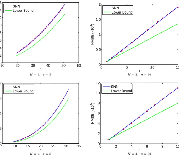
Empirical estimates of the statistical dimension. As noted in Theorem2.12, the statistical dimension of the descent coneδ(C)plays a crucial role in deriving our lower bound for the number of generic measurements. In the following, we will numerically justify our theoretical result forδ(C)under the setting of our interest, low-rank tensors.
ConsiderX0as aK-moden×n× · · · ×n(super)diagonal tensor with only the firstrdiagonal entries as
1and0elsewhere. Clearly,X0∈Tr,and Corollary2.6, Theorem2.12and expression (2.3.20) yield
δ(C) :=δ C K X i=1 X(i) ∗, X0 !! ≥rnK−1−2, and δ(C) = Θ(rnK−1). (2.3.21)
In the following, we will numerically corroborate (2.3.21) based on recent results developed in statistical decision theory.
In order to estimateδ(C), we construct a perturbed observationZ0=X0+σG, where vec(G)is a standard normal vector andσis the standard deviation parameter. Then
ˆ X := arg min X kZ0−XkF s.t. K X i=1 X(i) ∗≤Kr= K X i=1 (X0)(i) ∗, (2.3.22)
can be computed as an estimate ofX0. Due to the recent results from Oymak and Hassibi [OH16], the normalized mean-squared error (NMSE), defined as
NMSE(σ) := E ˆ X −X0 2 F σ2 , (2.3.23)
is a decreasing function overσ >0and
δ(C) := lim
σ→0+NMSE(σ). (2.3.24)
Therefore, for smallσ,NMSEserves a good estimator forδ(C). For more discussions on related tensor denoising problems, see Section2.5.
In our experiment, we setσ= 10−8and for different triples of(K, r, n), we measure the empiricalNMSE averaged over10repeats. Dykstra’s Algorithm (see Section2.8.1) is exploited to solve the convex problem (2.3.22). Numerical outputs are presented in Figure2.2, which firmly conforms to our theoretical results displayed in (2.3.21).