EPRU Working Paper Series
2010-04
Economic Policy Research Unit Department of Economics University of Copenhagen Øster Farimagsgade 5, Building 26 DK-1353 Copenhagen K DENMARK Tel: (+45) 3532 4411 Fax: (+45) 3532 4444 Web:
Late Budgets
Asger L. Andersen, David Dreyer Lassen,
and Lasse Holbøll Westh Nielsen
Late Budgets
Asger L. Andersen David Dreyer Lassen Lasse Holbøll Westh Nielsen
Department of Economics, University of Copenhagen April 2010
Abstract
The budget forms the legal basis of government spending. If a budget is not in place at the beginning of the …scal year, planning as well as current spending are jeopardized and government shutdown may result. This paper develops a continuous-time war-of-attrition model of budgeting in a presidential style-democracy to explain the duration of budget negotiations. We build our model around budget baselines as reference points for loss averse negotiators. We derive three testable hypotheses: there are more late budgets, and they are more late, when …scal circumstances change; when such changes are negative rather than positive; and when there is divided government. We test the hypotheses of the model using a unique data set of late budgets for US state governments, based on dates of budget approval collected from news reports and a survey of state budget o¢ cers for the period 1988-2007. For this period, we …nd 23 % of budgets to be late. The results provide strong support for the hypotheses of the model.
Keywords: government budgeting, state government, presidential democracies, political econ-omy, late budgets, …scal stalemate, war of attrition
JEL codes: D72, H11, H72, H83
We are grateful to Jim Alt for comments, suggestions and advice regarding the data collection and we thank Alan Auerbach, Daniel Diermeier, Jim Snyder, Peter Norman Sørensen and participants in seminars and workshops at UC Berkeley, Copenhagen, Harvard, MIT, and University of Virginia and at the Public Choice meetings 2010 for comments. We thank Jim Poterba and Kim Reuben for sharing their data on revenue shocks with us. Anders Oltmann provided excellent research assistance. We gratefully ackonwledge funding from the program on Economic Policy in the Welfare State (WEST) at the University of Copenhagen.
1
Introduction
In the Summer of 2009, the state of California captured national headlines by failing to enact a budget before the beginning of the …scal year. In fact, the situation in California was so severe that the state could not meet its obligations and began issuing IOUs to cover payments to local governments, private contractors, and taxpayers. After 24 days of negotiations beyond the …scal year deadline between Republican governor Arnold Schwartzenegger and the Democratic-controlled state legislature, a budget was approved. California is not alone in …nishing its budget late: in 2009, eleven states failed to approve a budget before the beginning of the …scal year,1 and in our entire sample, which covers the 48 continental states in the years 1988-2007, 23% of all budgets were approved after the …scal year deadline. Delayed appropriations are even more common at the federal level: Meyers (1997) reports that in the period 1977-97, 68 percent of all federal appropriation bills were enacted after the beginning of the …scal year.
In state governments in the United States, as across all political arenas and at all levels of government, the government budget provides the legal foundation for government spending. If a budget is not approved and enacted by the beginning of the …scal year, the legal basis for government spending is jeopardized, and the consequences can range from a continuation of operations based on last year’s budget to partial government shutdown, depending on both speci…c constitutional provisions and the overall institutional framework.
Late budgets are an important object of study for three reasons: Economic costs, as a measure of legislative productivity, and as a measure of good governance. We address each in turn. First, when state governments are unable to enact a full budget before the beginning of a new …scal year, they often resort to passing temporary budget bills that allow appropriations for state government operations for a limited time only.2 Passing a temporary budget bill is not always possible, however, in some cases because of state laws,3 and in other cases because of
political con‡ict among state lawmakers. In the absence of a budget, many state governments …nd themselves in unknown legal territory. As a result, the consequences of budget delays vary considerably across states, and sometimes even from year to year within the same state. Some state governments stop paying their employees or withhold payments to state vendors and contractors, providers of Medicaid, school districts and local governments. In the most extreme cases, the state government shuts down all so-called "non-essential" services until a new budget is in place. In addition, the mere threat of a late budget means that state agencies,
1
These are Arizona, California, Connecticut, Delaware (by one day), Illinois, Michigan, Mississippi, New York, North Carolina, Ohio and Pennsylvania.
2
At the level of the federal government in the US, such bills are very common and known as "continuing resolutions." When such resolutions fail, the result may be government shutdown, witnessed most recently for the case of the US federal government in 1996; see Meyers (1997) for an account.
3
For an overview of procedures when the state budget is not passed by the beginning of the …scal year, see the National Conference of State Legislatures: http://www.ncsl.org/default.aspx?TabId=12616
school boards and local government must spend time developing plans for what to do if a stalemate extends beyond the end of the …scal year, whcih complicates planning and may lead to distorted decisions, such as hiring stops and hoarding of funds.4
Finally, state government creditworthiness may su¤er.5 In on-going, companion work (An-dersen, Lassen and Nielsen, 2010), we investigate the consequences of late budgets for, among other things, state borrowing costs. We …nd that late budgets are associated with higher state bond yields, as measured by the Chubb Relative Value Survey.6 Combining these estimates with state debt stocks, we …nd late budgets to be associated with substantial per capita interest rate premiums. In short, late state budgets have signi…cant economic consequences within as well as beyond state governments.
Second, our measure of budget negotiation duration provides a replicable, and easily ex-tendable, measure oflegislative gridlock, de…ned as the inability of the legislative and executive branches to pass major legislation, at the state level. While a major part of the literature on legislative gridlock has focsued on the US federal government (e.g. Mayhew, 1991; Binder, 1999), the logic behind the models and arguments applies to veto player democracies every-where (Tsebelis, 2002). There is no generally agreed-upon measure of legislative gridlock (see, e.g., Chiou and Rothenberg, 2008), but the budget arguably is the most important piece of legislation for any executive and legislature. As recognized by Mayhew (1991), and emphasized by Fiorina (1996) and Binder (1999), a true measure of gridlock should take into consideration both the supply and demand for legislation; while low legislative output could re‡ect high levels of gridlock, it could equally well re‡ect both a lack of demand for such output and a lack of supply due to less frequent introduction of bills in periods where chances of passage are lower. Our measure corrects for endogeneity both on the supply and the demand side, as the budget’s (re-)appearance on the legislative agenda is exogenously given.7
Third, timely budgets can, more generally, be viewed as a measure of good governance. In his analysis of the e¤ects of social capital and the civic community on governance outcomes, Putnam (1993) includes as one of his twelve indicators of institutional performance budget
4
In Maine in 1991, 10,000 state government workers were sent home without pay and all non-essential services were closed. The budget was 18 days late. In Illinois, delays in payments from the state government creates problems of liquidity for counties (“County copes with cash ‡ow", Lincoln Courier, April 8, 2010). In Michigan, late state budgets a¤ect sta¢ ng and tuition decisions at schools and universities (Citizens Research Council of Michigan: Late Budgets in Michigan, August 2009).
5
On July 6, 2009, a few days after the beginning of the …scal year, Fitch Ratings dropped California’s bond rating to BBB, down from A minus (Wall Street Journal, July 8, 2009: Big Banks don’t want California’s IOUs).
6
The measure is based on a survey, carried out by the Chubb Corporation, of sell-side bond traders who are asked to rate the relative yield on a 20 year general obligation bond for a state icompared with a similar bond issued by New Jersey. See Lowry and Alt (2001) and Poterba and Rueben (2001) for more on the Chubb Relative Survey and Andersen, Lassen and Nielsen (2010) for the analysis.
7
Obviously, by restricting ourselves to studying budgets as a venue for gridlock, we leave out many important policy areas; however, little agreement exists in the literature (Chiou and Rothenberg, 2008) on how to measure major bills.
promptness, de…ned as the (lack of) delay relative to the beginning of the …scal year of the approval of the budget by the regional councils. Putnam (1993, p. 65-67) argues that budget promptness is a measure of a government’s “essential internal a¤airs” which, in turn, is one component of an evaluation of good government.8 Our rich panel data set allows us to include measures of social capital alongside economic and political explanatory variables to assess their relative importance in explaining late budgets.
A …nal reason for studying late budgets is methodological in nature: Empirical analyses of budget outcomes and …scal stabilizations are almost always based on models of political bargaining, often involving a number of veto players, but the analyses are rarely based on data on the actual bargaining process. As such, studies based on real-world data linking institutions to outcomes by way of bargaining are essentially estimating reduced form-relationships by stipulating an unobserved bargaining process, weakening the link between the proposed theory and the empirical results. In contrast, our approach makes the bargaining process the center of the analysis with the aim of evaluating directly the hypoteses about the bargaining solution derived from the theoretical model.
We model the political bargaining proces as a war of attrition in the spirit of Alesina and Drazen (1991), but we focus on the time to reach an agreement on the annual budget rather than the delay in implementing crises-induced reforms. In our model, the two bargaining parties su¤er costs from not being able to reach a deal. These costs may be political of nature, because the public dislikes budget delays, or they may be personal, since legislators must spend time and e¤ort to keep battling over the budget. When a party …nds that it can no longer bear the costs of continued bargaining, it concedes, and the opposing party is free to implement its preferred policy. We derive the unique symmetric equilibrium of the bargaining game and show that it implies a number of testable hypotheses. The three main predictions are: One, changes in …scal circumstances, regardless of direction, increase the expected duration of budget stalemates; Two, the expected duration is higher in …scal downturns than in upswings of similar magnitudes; And three, divided government increases the expected duration.
Our modeling approach is based on the key assumption that bargaining over a government budget is carried out with reference to a budget baseline. Budget baselines generally fall in two categories: (1) nominal spending the previous year; or (2) “current services” which is the provision of services …nanced by the previous year’s spending. In US state governments, which form the focus of our empirical analysis, Crain and Crain (1998) report that in the 1990’s 34 states used last year’s spending level as baseline while the remaining 16 used a current services baseline. While the determination of baselines themselves is also subject to political
8This sentiment is echoed among policy makers; for example, Scott Pattison, the current executive director of the National Association of State Budget O¢ cers, notes that "a well-managed state would never, ever" have a late budget (quoted from "Mischief After Midnight", governing.com, June 2009. Available online at http://www.governing.com/article/mischief-after-midnight).
manoeuvring and debate, a baseline remains, given the baseline regime, a common reference point against which all changes being bargained over are compared; as noted by Schick (2007, p. 67) in the context of the US federal government budget, “[o]nce a baseline has been constructed, any variance from it due to legislation is measured as a policy change.”
We combine the notion of a formalized reference point in the form of a budget baseline with the behavioural assumption that budget negotiators have political preferences and that they are loss averse over changes from the baseline, making the preferences a variant of Tversky and Kahneman (1991). It is well documented that public responses to negative economic informa-tion is greater than responses to positive informainforma-tion (Soroka, 2006), that negative attitudes towards candidates have a greater impact on voting behavior than do positive attitudes (Ker-nell, 1977), and that negative economic trends penalize incumbents while they reap few bene…ts from positive trends (Bloom and Price, 1975; Nannestad and Paldam, 1997). These observa-tions are in accord with the di¤erential valuation of negative and positive political outcomes reported in Quattrone and Tversky (1988), suggesting that voters exhibit loss aversion over goods, services and transfers obtained from the public sector. We do not model the relation-ship between voters and politicians; instead, we directly assume politicians to be loss averse, which can either simply re‡ect loss averse voters or re‡ect the fact that politicians themselves are subject to the same processes of preference formation as are voters. Loss aversion implies a status quo bias (Samuelson and Zeckhauser, 1988), or - in our model - more precisely, a bias towards the baseline budget. This means that the opposing parties in our model …nd it relatively easy to agree on keeping the budget unchanged in years when …scal conditions are stable. When exposed to large changes in …scal circumstances, however, their innate di¤erences in policy preferences make the parties disagree over how to adapt to such changes, and long stalemates become more likely. Because of loss aversion, this is more pronounced when …scal conditions change for the worse than when they improve.
We apply the model to data on US state government budget processes. Using state and local newspaper sources as well as responses to a survey of state budget o¢ ces administered for this purpose, we collect data on dates of …nal budget enactment and compare these to the beginning of the state governments’ …scal years. Carrying out this comparison for all states for every year since 1988 yields a replicable measure of budget lateness (as well as legislative gridlock and governance).9
We …nd that adverse changes in economic conditions, measured by the increase in unem-ployment, substantially increases the duration of the budget negotiations: a one percentage point increase in unemployment rate relative to the previous year increases the expected
du-9The Government Performnace Project at Pew Center of the States provides overall assessments of government performance to produce an index of same. This index was employed by Knack (2002) in his cross-state analysis of the e¤ects of social capital on governance. ’Budget timeliness’is one of many factors included in this assessment, but it is not reported separately nor is it based on hard data.
ration of the budget negotiations by about a week in our preferred speci…cation. Similarly, divided government substantially increases both the risk of experiencing a late budget and its duration, the latter by about two weeks. On the other hand, budget negotiations are, on average, between one and two weeks shorter in election years.
The paper is structured as follows: The next subsection presents related literature, section 2 presents our theoretical model, and section 3 describes the collection and construction of data. Section 4 describes the empirical speci…cation and section 5 reports results. We provide a discussion and some concluding remarks in the …nal section.
1.1 Related literature
Our study of late budgets relates to a number of di¤erent literatures, in addition to the leg-islative gridlock and good governance literature already mentioned. First, it is related to the political reform literature, in particular the literature on …scal adjustments in the face of large, external shocks. This is evident not only from the descendancy of the model from the Alesina-Drazen framework, but also from the fact that budget lateness, as will become evident from the empirical analysis, is crucially related to an adverse economic environment and speci…c political factors. However, the theoretical and empirical literatures on …scal adjustments are not concerned with annual budgets per se, but with …scal imbalances over the medium- and long-term, and have as a key parameter the economic costs of continuing con‡ict.10 In contrast,
we set up a framework to cover all budgets, in normal times and economic crises alike, based on political costs of bargaining rather than economic costs, and provide empirical evidence to match the theory closely.
Second, our study is a part of the large literature on the e¤ects of political, economic and institutional determinants of government budget outcomes. In this literature, government budget outcomes, i.e. realized revenue and spending patterns, are related to partisan di¤erences (Alt and Lowry, 2000), budget institutions (Poterba, 1994; Alt and Lowry, 1994; Poterba and von Hagen, 1999) and political institutions (e.g. Grossman and Helpman, 2007). While most theoretical work in this literature explicitly recognizes the bargaining nature of government budgeting and policy determination, direct empirical tests based on quantitative data of the theoretical claims regarding the bargaining process are, to our knowledge, non-existent.
Third, our paper is related to the concept of incrementalism as well as to the general public administration literature on budgeting. Incrementalism in budgeting is traditionally associ-ated with Wildavsky’s (1964) observations that government budgets are not re-calculassoci-ated from scratch every year but that they are rather, due to information processing costs, based, by-and-large, on the previous year’s budget. Our approach, based on budget baselines as points
1 0
In a recent contribution to this literature, Alesina, Ardagna and Trebbi (2006) provide an investigation of the determinants of …scal balance stabilizations across countries.
of departure for budget negotiations, is not derived from incrementalism; if anything, as noted by Schick (1980, p. 217), the adoption of the current services baseline institutionalized incre-mentalism.11 The role of the status quo and agenda control in models of policy determination
was …rst recognized by Romer and Rosenthal (1978).
Fourth, the paper is closely related to a small literature studying bargaining in positive analyses of political and policy processes. Bargaining models are frequently employed in the positive political economy literature, but, as noted above, most empirical studies go on to evaluate economic and political outcomes directly, rather than studying the bargaining process by which exogenous circumstances are translated into outcomes. Analyses linking formal bar-gaining models to data on the barbar-gaining process are rare outside of laboratory experiments, but notable exceptions exist: Merlo (1997) and Diermeier, Eraslan and Merlo (2005) exam-ine government formation in Italy and parliamentary democracies, respectively, based on the stochastic bargaining model proposed by Merlo and Wilson (1995). The duration of the gov-ernment formation phase can be interpreted as a measure of the intensity of the con‡ict, as can the duration of the budget negotiation phase.
2
A Stylized Model of Budget Delays
We consider a government with two players,A and B, who must agree to pass a budget. The players could be thought of as the executive vs. the legislature, or as majority leaders from di¤erent chambers within the legislature. Each player has veto power, so that no one player can pass a budget without the consent of the other player.
The government faces a given amount of revenue, y, which can be spent on two di¤erent types of publicly provided goods, g1 and g2. There is a balanced budget constraint in place,
so any budget plan must satisfy g1+g2 = y. All variables are measured in units per capita.
The players derive utility from both types of spending, but they disagree on the preferred composition of total spending. An alternative interpretation is thatg1 and g2 are public- and
private consumption, respectively, and thatyis the tax base, assumed for simplicity to be equal to income per capita. The tax rate is then equal to g1=y. In this interpretation, the con‡ict
between the two players is over the size of the budget, rather than the composititon. Which of these two alternative interpretations is the appropriate one depends on the relevant context in which we wish to apply the model’s predictions. However, for consistency, we stick to the …rst interpretation in the following exposition.
The political game resembles the set-up in Alesina and Drazen (1991): The two players engage in a war of attrition, during which the budget adoption is delayed. Delaying agreement
1 1
The debate over incrementalism and alternative public administration models of budgeting cannot be done justice here. For a critique of incrementalism, and an alternative budgetary theory, see Meyers (1996).
is costly to both players. First, budget delays imply a political cost to those responsible, since voters disapprove. And second, there is a personal cost of delay to the players involved, since they must spend time and resources on negotiating, lobbying and servicing the press as long as the adoption phase continues.
There may also be actual budgetary costs associated with delays. As explained above, government agencies must spend time and e¤ort to deal with the delayed appropriations and the possibility of shutdown of services, and this may divert resources away from provision of public goods and services. This would suggest a negative relationship between the duration of the delay andy in our model. However, to keep things simple we focus on the …rst two types of costs of delay and let y be constant over time.
The war of attrition ends when one of the players "concedes". We model our political con‡ict as a "winner-takes-all" game: once a player has conceded, the other player is free to choose whatever composition of spending he prefers. Thus, as in Alesina and Drazen’s model, players can only "win" or "lose". Endogenously determined compromises reached during negotiations are ruled out, which is of course a major simpli…cation.12
The players have reference-dependent preferences, so that budget outcomes (g1; g2) are
evaluated relative to a budget baseline,(g1b; g2b). To be speci…c, we assume that their preferences over government spending can be represented by the utility functions
uA(g1; g2jgb1; g2b) = v(g1 gb1) +v(g2 gb2) (1)
uB(g1; g2jgb1; g2b) = v(g1 gb1) + v(g2 gb2)
where
v(x) = x if x 0
x if x <0 and > >1
The parameter captures that each player prefers spending on one type of good over the other, other things equal, but they disagree on which of the two goods is preferable. With
>1, player A has a preference for spending on good 1, while player B prefers spending on good 2. The players evaluate budget outcomes in terms of deviations from the baseline, using the value functionv( ). The value function is everywhere increasing and has a kink at zero, as suggested by Tversky and Kahneman (1991).13 This implies that the players are loss-averse: They dislike negative deviations from the baseline more than they like equal-sized positive deviations.
1 2
Hsieh (2000) provides an extension of a simpli…ed Alesina-Drazen framework where the payo¤ distribution at stabilization is determined endogenously in a formal bargaining process.
1 3
Tversky and Kahneman also argued that in order to explain observed attitudes towards risk, the value function must be concave in the positive domain and convex in the negative domain. This feature of the value function is known asdiminishing sensitivity. Since we are not explicitly interested in explaining attitudes towards risk, we abstract from this feature and settle for the simpler, linear version adopted here.
To see what our speci…cation of preferences implies for budget outcomes, de…neyb g1b+g2b. We label this the baseline revenue level. When y > yb the players face an opportunity to raise spending on both types of goods over the baseline levels. Since > 1, player A gets higher marginal utility from raisingg1 than from raisingg2 whenever g2 g2b. Hence, playerA would
never raise spending on good 2 above the baseline level. On the other hand, the assumption
> implies that player A does not wish to driveg2 below its baseline level. Player A thus
prefers the bundle(g1b+y yb; g2b)to all other feasible combinations ofg1 and g2 wheny > yb.
Correspondingly, the marginal bene…t to playerAfrom raisingg1at the expense ofg2is positive
when g1 < g1b and g2 < gb2, but negative when g1 g1b and g2 < gb2. If given the opportunity,
player A will therefore choose the bundle (gb1; g2b yb+y) when y < yb. Of course, player B’s preferences imply the same choices, only with the goods reversed.
In words, whenever the players are given an opportunity to raise overall spending, they will prefer to increase spending on their preferred good only, while leaving spending on the other good unchanged. And whenever faced with a need to cut overall spending, the players will prefer to keep spending on their preferred good unchanged, letting spending on the least preferred good carry the entire burden of adjustment.
The assumption > is crucial for these results. Without this assumption, both players would always prefer to spend the entire revenue on their own preferred good, irrespective of the sign of y yb. The interpretation is that the players are so averse to losses that they are willing to sacri…ce increases in spending on their most preferred good in order to avoid even the smallest cuts in spending on their least preferred good. Of course, this is an extreme prediction. However, we believe that it does capture an important feature of …scal policy: Spending cuts carry a greater weight in the minds of citizens, in the public debate, and therefore also in the minds of policymakers, than spending increases. Fiscal policymakers are therefore inclined to avoid spending cuts, even at substantial opportunity costs.
The costs from a stalemate over the budget are individual-speci…c and linearly increasing in the time until a concession occurs. Time is continuous and we normalize the start of the budget adoption phase to t= 0. If a concession occurs at time t=T, the players incur disutility
Di = iT ; i=A; B (2)
The parameter i captures how costly delays are to player i. We assume that A and B
are independent and drawn randomly from a uniform distribution on an interval ( ; ]. As in Alesina and Drazen (1991), we assume that i is private information to player i. The other
player does not observe the realized value of i but knows the distribution from which it is
drawn.
delayed agreement. If player i ultimately wins the war of attrition at time t = T, his total utility may then be written as
UiW(T) =uW Di(T) =
(y yb) iT if y yb
(yb y)
iT if y < yb
(3) while the total utility of losing at timeT is
UiL(T) =uL Di(T) =
(y yb) iT if y yb
(yb y)
iT if y < yb
(4) The gain from winning is then straightforwardly computed as
UiW(T) UiL(T) =uW uL= ( 1)(y y
b) if y yb
( 1)(yb y) if y < yb (5)
Note that the gain from winning is always positive, equal for both players and independent of the time of concession. It is increasing in y yb , the absolute value of the deviation of total revenue from its baseline. Note further that for a given value of y yb , the gain from winning is higher ify < yb than ify yb: because of loss aversion, the stakes are higher when revenue drops below the baseline level than when it is above it.
Each player must now choose an optimal concession time Ti. This is the date on which
player i concedes and allows his opponent to choose her preferred spending plan, conditional on the opponent not having conceded already. We assume that players choose Ti so as to
maximize their expected total utility. Expected utility depends on the utilities that the player gets from winning and losing, respectively, as well as the probability of winning. Player i
wins whenever his chosen concession time exceeds that of his opponent. Let H(t) denote the cumulative distribution function of the opponent’s optimal concession date, with associated density function h(t).14 H(t) is of course endogenous, but it is exogenous as seen from the
point view of playeri, since playerican in no way in‡uence his opponent’s choice of concession time. Integrating over the opponent’s concession time, we can then express the expected utility
1 4As emphasized below, we concentrate on equilibria where each player’s concession time is a di¤erentiable function of his type. This implies that H(t) is di¤erentiable, and that the density functionh(t) does in fact exist.
of playerias a function of Ti as EUi(Ti) = Ti Z 0 UiW(t)h(t)dt+ 1 Z Ti UiL(Ti)h(t)dt (6) = Ti Z 0 UiW(t)h(t)dt+ (1 H(Ti))UiL(Ti)
If a positive, …nite optimal concession time exists, it must then satisfy the …rst-order con-dition
dEUi(Ti)
dTi
= UiW(Ti) UiL(Ti) h(Ti) (1 H(Ti)) i = 0 (7)
where we have used that@UiL(Ti)=@Ti= i. Recall that the term in brackets is the gain from
winning, which does not depend onTi. We may therefore write this term asuW uL. We can
then rewrite the …rst-order condition as
[uW uL] h(Ti)
1 H(Ti)
= i (8)
This representation of the …rst-order condition has an intuitive interpretation: The left-hand side is equal to the expected marginal bene…t of waiting one more instant to concede. This is equal to the probability that the opponent will concede "within the next instant", conditional on the fact that he has not already conceded, times the gain that follows if the opponent does actually concede. The left hand side is equal to the marginal cost of postponing concession. At the optimal concession time, the marginal bene…t and the marginal cost exactly balance.
We now look for a symmetric Bayesian Nash equilibrium in which each player’s optimal concession time Ti is a di¤erentiable function of his type, Ti = T( i). In the appendix we
show that there exists a unique such equilibrium. The equilibrium function T( i) satis…es the
di¤erential equation
T0( i) = [uW uL]( i( i )) 1 (9)
and the boundary condition
T( ) = 0 (10)
Combining equations (9) and (10) then gives the following explicit solution for T( i):
T( i) = uW uL 1
ln i( )
( i )
(11)
solu-tion. More precisely, we may back out the equilibrium distribution by noting that H(t) =
P rob[T( j)< t] =P rob j > T 1(t) , whereT 1 is the inverse function to T.15
To understand the mechanisms of the game in the symmetric equilibrium, recall that when deciding whether to concede or keep …ghting, the players weigh the expected marginal bene…ts of a further delay against the marginal costs, i. The marginal bene…t consists of the conditional
probability that the opponent will concede "within the next instant", times the gain from winning that follows if he actually does so. In the beginning of the con‡ict, this marginal bene…t can be shown to be exactly , implying that no player with i < will concede immediately.
However, since opponents with high costs from delays will concede faster, the passage of time without a concession makes players adjust their beliefs about their opponent’s costs downwards. With the speci…c distributional assumption we have made about costs, it also implies that the conditional probability that the opponent will concede within the next instant falls.16 Thus,
the marginal expected bene…t of postponing concession decreases over time, and after a certain time it becomes so low that equation (9) exactly holds. This is the optimal time for player i
to capitulate and accept defeat.
A budget agreement is reached as soon as one of the players concedes. The date when this happens is given by
Tagree = minfT( A);T( B)g
Of course,Tagree is a random variable. Using equations (11) and (5), and the fact that Aand B are independent and both uniformly distributed on( ; ], we show in the appendix that the
expected date of agreement is
ETagree = ( 1)(y y
b) if y yb
( 1)(yb y) if y < yb (12)
where (ln( ) ln( )) ( ) 2.
2.1 Predictions from the model
A number of predictions are immediately apparent from equation (12). First, large deviations in revenue from the baseline level increase the expected time until concession. Since baseline budgets are strongly linked to the previous budget, it follows that we should expect changes in …scal circumstances relative to the previous year, whether to the better or worse, to increase the expected duration of budget stalemates. The intuition is that in years when revenue is
1 5The appendix also proves that the functionT is strictly decreasing, so that the inverse function does exists. 1 6
This conditional probability is equal to the hazard rate,h(T)=(1 H(T)). The assumption that the i’s are
stable, reference dependence and loss aversion imply that both players prefer to keep spending levels unchanged. This consensus between players, which arises despite their innate di¤erences in preferences, means that there is little at stake in the con‡ict over the budget, and both players will therefore prefer to concede quickly, rather than dragging the stalemate to a length and incur the political costs associated with the delay. In contrast, in the face of large changes in …scal conditions, the players disagree on how to adapt to those changes. This increases the stakes in the budget con‡ict, and the opposing parties will be more willing to prolong the stalemate in the hope of getting their preferred outcome.
Second, negative deviations from the baseline have a stronger impact on the expected time of concession than positive deviations of the same size. Hence, the model suggests that we should observe longer budget delays during …scal downturns than during upswings. This prediction follows directly from the assumption of loss aversion: since players dislike spending cuts more than they like spending increases, it becomes extra important for them to control the budget in years where revenue has dropped. Loosely formulated, "avoiding to lose" is a stronger motivation to keep …ghting than "hoping to win".
Based on the …rst two predictions, we should expect to see longer and more frequent budget delays in states where revenue is highly volatile. On the other hand, it is the need for spending to adapt to changes in revenue, not the change in revenue in itself, which leads to delays in our model. Going slightly outside the model, we would therefore expect …scal institutions that facilitate smoothing of ‡uctuations over time to dampen the impact of revenue volatility.
A third prediction relates to the parameter . The larger is, the stronger are the players’ relative preferences for their favored types of spending, and the deeper is their disagreement over how to react to a change in revenue from the reference level. = 1 corresponds to a com-plete consensus on the budget, in which case the model predicts immediate agreement always. Naturally, signi…cant discrepancies between the policy preferences of the players involved in the budget process are much more likely when there is divided partisan control of the government than when all players belong to the same party. Thus, we expect budget stalemates to be longer and more frequent when the two chambers in the legislature are controlled by di¤erent parties, or when the legislature is controlled by the opposite party of the executive.
Finally, the expected date of concession is inversely proportional to the scale of the interval
( ; ]. That is, multiplying and with a positive constantkimplies thatETagreeis multiplied
with k 1. Similarly, adding a positive constant to both and lowers ETagree.17 Hence, a
shift to the right in the distribution of the marginal costs of delay leads to shorter expected stalemates. We therefore expect to see shorter delays when the political and personal costs to
1 7To see this, totally di¤erentiate equation (12) with respect to and and set d = d . This gives dETagree=d = [UW UL]( ) 2( ln( ) 1) < 0. The term in the parentheses is positive since
politicians of late budgets are high. This may for example be the case in election years: First, electoral success is likely to depend on recent performance, so the political costs of delays are extra high in such years. And second, legislators face an extra personal opportunity cost of spending time on battling over the budget in election years, since they cannot devote their time to campaigning for re-election until the budget is done. Institutional arrangements may also in‡uence the political and personal costs of budget delays, an issue that we address further in the empirical analyses below.
3
De…ning and measuring late budgets
Budget processes vary considerably across US states. This complicates cross-state comparisons of budget timeliness somewhat, since there is no obvious, universal de…nition of when, and by how much, a budget is late. For any meaningful measure of budget lateness, one must identify two points in time, namely 1) the date by which the budget is supposed to be enacted; and 2) the date on which it is actually enacted. To begin with the former, many state legislatures face a deadline to pass the budget that is prior to the end of the …scal year. For example, the California state constitution requires that the legislature pass the budget bill before June 15, whereas the …scal year starts on July 1st. Other state legislatures face constitutional or statutory deadlines for ending their regular sessions. Whether such deadlines also constitute an e¤ective deadline for passing the state budget varies from state to state, however, and is often a question of interpretation. Moreover, while violations of pre-…scal year deadlines are often met with harsh criticism in news media, most of the political and economic costs of a budget stalemate that we discussed in the introduction do not become relevant until the stalemate approaches the end of the …scal year. Most notably, government shutdowns can only happen if the impasse extends into the new …scal year. In our view, therefore, the ultimate deadline for enacting a state budget will always be the end of the …scal year.
Turning to the date of actual budget enactment, two natural candidates come to mind: the date of …nal legislative approval and the date of …nal enactment. Final legislative approval is achieved when the new budget has been passed in both chambers of the legislature in its …nal form. Final enactment is the event that formally makes the new budget become law. In most cases, this happens when the governor signs the budget, but important exceptions exist: For example, if the governor vetoes the entire budget, the legislature can in most states override the veto by some super majority vote in both chambers, and the budget then becomes law without the governor’s signature. In such cases we interpret the date of the legislative override as the date of …nal enactment. Furthermore, some states have a deadline for gubernatorial action, and the governor may sometimes let the budget become law without actively signing it
by letting this deadline expire. In these cases we use the date on which the deadline expired.18 For convenience, however, we shall henceforth simply refer to the date of …nal enactment as the date the budget was signed into law.
It is not obvious which of the two events most accurately captures the end of budget negotiations. Sometimes, all con‡ict is e¤ectively resolved when the budget has been passed by both legislative chambers, and the governor’s signature appears to be a mere formality. This speaks for using the date of legislative passage as the indicator of actual budget enactment. In other cases, however, the con‡ict over the budget is far from resolved with the legislative passage. Many governors actively use their power to veto the budget - or the threat to do so - to in‡uence the …nal budget outcome. In such cases, the …nal budget enactment, i.e. the signing into law, is the appropriate indicator for the end of budget negotiations. Since this is also what formally marks the end of the budget adoption process, we prefer the date when the budget is signed into law as our indicator of budget enactment.19
Thus, our preferred measure de…nes a late budget as a budget that has been signed into law after the end of the …scal year, and we measure the length of the delay as the number of days from the end of the old …scal year to the date of …nal enactment. We have also experimented with two other measures, however, namely 1) the number of days from the state-speci…c deadline for legislative passage of the budget to the date of actual legislative passage, and 2) the number of days from the end of the old …scal year to the date of legislative passage.
3.1 Budget enactment data
The data for the budget enactment dates were collected from three sources: (i) State leg-islatures’ websites; (ii) Archived newspaper articles; and (iii) a survey sent to state budget o¢ cers. Some state legislatures’websites have detailed information on the status and histories of all bills enacted in previous legislative sessions, including the budget bill(s). However, most state legislatures’bill tracking tools only cover the most recent legislative sessions, if any. We therefore supplemented with information from archived newspaper articles accessed via Newsli-brary.com.20 Finally, we also sent a survey to state budget o¢ cers asking them to con…rm the
1 8
Another exception is Maryland, where the governor cannot veto the budget, which means that the budget becomes law once it has been passed by both chambers in the legislature. Consequently, …nal legislative passage and …nal budget enactment coincide in Maryland.
1 9Our measurement is further complicated by the fact that some states do not pass a single, all-encompassing budget bill. Instead, their budgets consist of several individual appropriation bills. In such cases we do not consider the budget fully enacted until the last appropriation bill for state operations has been enacted. Also, state governments sometimes react to unexpected developments in state government …nances by passing within-…scal year supplementary appropriation bills. We do not view such supplementary budget bills as part of the budget adoption process that we are interested in, however, and we therefore restrict our attention to the budgets as originally enacted.
2 0Newslibrary.com is an online newspaper archive that covers more than 2,500 news sources across the United States. We also used The New York Times online archive on several occasions to access relevant news articles.
data we had collected ourselves as well as provide us with the information that we had not been able to …nd via any of the other sources. Out of 48 states (we exclude Alaska and Hawaii), 19 responded to our survey. When overlapping, the data they reported were virtually identical to the data we collected ourselves.21
In the survey, as well as in our own information search, we asked the following questions for each legislative session in which a budget was adopted:
1. When did the regular session of the legislature start?
2. When was the executive budget proposal submitted to the legislature? 3. When was the deadline for the legislature to pass the budget?
4. When did the legislature pass the budget? 5. When was the budget signed into law?
Our main dependent variable,days_late, is constructed as the di¤erence between the answer to question 5 and the last day of the old …scal year. Note that this variable is uncensored, so that both positive and negative values occur. For example, a value of days_late equal to -5 means that the budget was signed into law …ve days before the end of the …scal year. We also construct a binary variable, late_budget; that takes the value one if days_late is strictly positive, and zero otherwise. In addition, we construct a censored variable, days_late_cens, that sets all negative values equal to zero. Our two alternative measures, days_delayed; and,
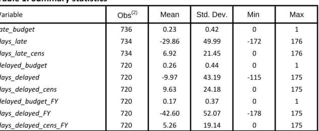
days_delayed_F Y, are constructed as the di¤erence between the answer to question 4 andi) the answer to question 3, and ii) the last day of the old …scal year, respectively. Binary and censored versions of these variables are constructed in a similar way. Table 1 shows descriptive statistics for all dependent variables.
<Table 1 about here[Descriptive statistics of dependent variables]>
For the years 1988-2007 we have recorded 167 cases where the budget was signed into law after the beginning of the new …scal year. This amounts to 23 percent of the budgets for which we have data.22 Figure 1 gives a detailed picture of the distribution of days_late. There is a clear e¤ect of the …scal year deadline, as can be seen from the spike at zero. This spike re‡ects the great number of budgets that are enacted on the last day of the old …scal year. The
2 1
The instructions for the survey are available from the authors upon request. Table A1 in the appendix gives details on the source of information on late budgets for each state.
2 2
190 budgets (26%) received legislative passage after the legislature’s state-speci…c deadline, while 119 (17%) were …nally passed by the legislature after the beginning of the new …scal year.
budgets that were signed into law after the beginning of the new …scal year (days_late >0) were on average 31 days late. The variation is large, however, ranging from one day to almost six months with a standard deviation of 36 days. 13 percent of the late budgets were signed into law on the …rst day of the …scal year, while 33 percent were more than one month late.
<Figure 1 about here. [No. of days from end of …scal year to …nal budget enactment]>
Figure 2 illustrates the occurrences of late budgets over time. In addition to our preferred de…nition of a late budget, the …gure also displays the number of budgets that were passed by the legislature after the state-speci…c deadline for legislative passage. Such delays are generally much more common than delays that extend into the new …scal year. For both measures, budgets delays were frequent in the early 1990s and in the beginning of the new century. The late 1990s were a period with relatively few late budgets.23
<Figure 2 about here. [The number late budgets over time, 48 states]>
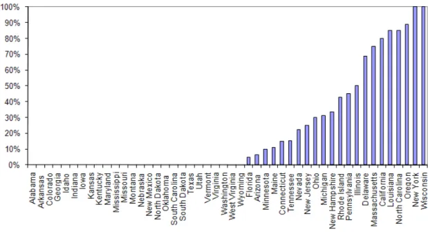
Figure 3 illustrates the relative frequencies of late budgets for each of the 48 states in our data set, using our preferred de…nition of a late budget (days_late >0). In comparison, Figure 4 does the same for one of our alternative de…nitions (days_delayed > 0). Most states have experienced at least once that the state legislature didn’t live up to its deadline for budget passage, while 22 states have experienced a budget enacted after the beginning of the new …scal year in the time period considered here. New York, North Carolina, California, Oregon and Wisconsin score high on both measures of budget lateness, while Southeastern, Plains- and Rocky Mountain states dominate the group that have never experienced any late budgets.
In what follows, we report results for our preferred de…nition of late budgets only. Table A3 in the appendix reports results for our main explanatory variables of interest using the two alternative de…nitions. A full set of results that parallel those reported below are available from the authors upon request. In short, all of our main conclusions are highly robust to plausible alternative de…nitions of a late budget.
<Figure 3 about here.[No. of budgets enacted after beginning of …scal year, relative to total no.
of enacted budgets 1988-2007]>
<Figure 4 about here:[No. of budgets passed after legislature’s deadline, relative to total no. of
enacted budgets 1988-2007]>
2 3
Note that odd years generally have more late budgets than even years. This is due to the fact that almost all states with biennial budgeting pass new two-year budgets in odd years, so more budgets are enacted in odd years than in even years. Relative to the total number of budgets being enacted, there is no di¤erence between odd years and even years.
4
Explanatory variables
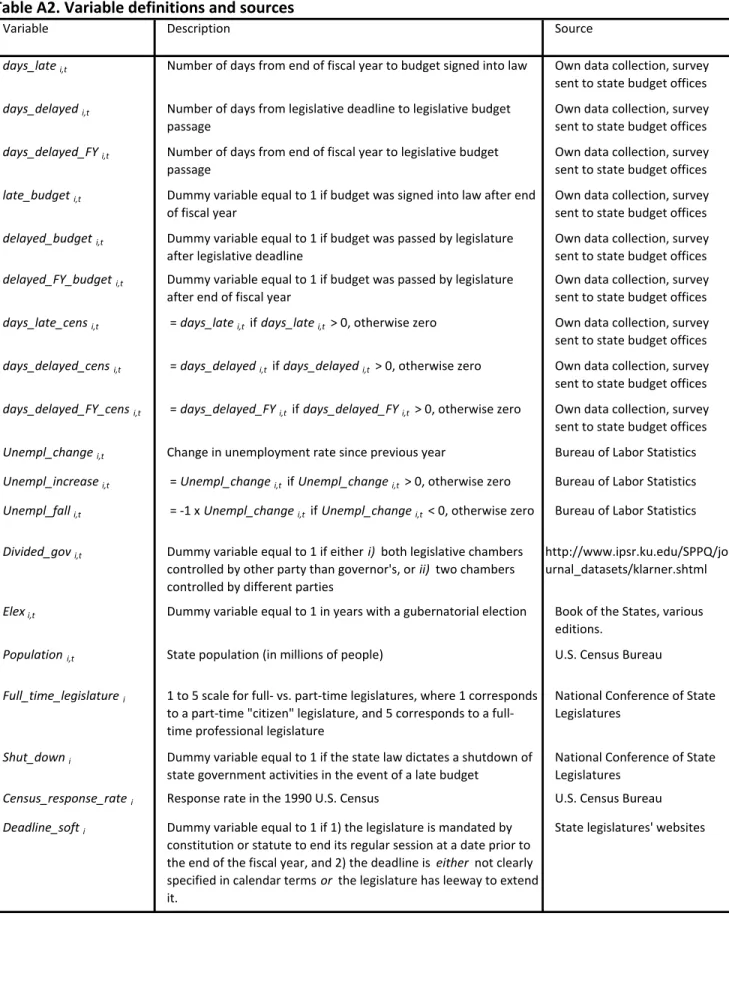
This section describes the set of explanatory variables in our empirical analyses. More detailed descriptions of all variables, including their sources, can be found in table A1 in the appendix. A key prediction of the model is that a shock to the …scal climate (as compared to the previous year) should lead to a delay in the budget adoption, with the delay being longer, the greater the shock is. To test this prediction, we include di¤erent measures of changes in the …scal climate in our estimations. Our preferred measure is the change in the state unemployment rate compared to the previous year. An important advantage of this measure over other candidates is that unemployment statistics are typically available with a much shorter time lag than, say, growth rates in state GDP. Thus, the state unemployment rate is likely to re‡ect the information available to policymakers at the time of budget adoption more accurately than other measures of the business cycle. Furthermore, Scheppach (2009, p. 1) notes that "the trough in state revenue generally coincides with the peak in unemployment". Finally, the change in the state unemployment has the nice property that there is a natural distinction between positive shocks to the …scal climate (decreases) and negative shocks (increases).24 We also consider an alternative measure that focuses more directly on …scal conditions, namely the revenue schock measure developed in Poterba (1994) and Poterba and Rueben (2001).
As explained above, we expect divided control over the state government to produce longer and more frequent budget delays. We therefore include a dummy variable that takes the value one if either i) both chambers in the legislature are controlled by another party than the governor’s (split branch), or ii) the two chambers are controlled by di¤erent parties (split legislature):We shall later look more into the di¤erence between these two types of divided government.
An additional prediction of the model is that the greater the cost politicians incur during delays, the shorter is the expected delay. As mentioned in section 2, we expect such costs to be higher in election years than in non-election years. We also consider measures that plausibly correlate with the opportunity cost of budget stalemates for the politicians involved: Part-time legislators often have well-paid civil occupations in addition to their political o¢ ce, and they typically receive only a modest compensation (and perhaps none at all if the deadline is exceeded) for spending time at the state assembly. Hence, part-time legislators have a much greater opportunity cost of delaying agreement than full-time legislators, who have no or limited outside occupation. We therefore include a variable that characterizes the state legislature on a 1 to 5 scale, where 1 corresponds to a part time "citizen legislature, while 5 corresponds to a full-time professional legislature. Our prior is that delays are both longer and more frequent
2 4
No equally natural distinction exists for another potential measure, namely the growth rate in real state GDP; what constitutes a negative shock in this case? A negative growth rate? A below-average growth rate? Or a drop in the growth rate relative to last year? In our opinion, there is no obvious answer to this question.
in full-time legislatures.
In a similar spirit, we also include dummy variables for whether the legislature is required (by constitution or statute) to end its regular session before a certain deadline. Where such deadlines are present, a failure to pass the budget before the deadline means that the legis-lature must go into overtime session, or that a special session must be called. This increases the salience of budget impasses, and we therefore expect the political costs of proctracted ne-gotiations to be higher in states that have such deadlines. We distinguish between two types of legislative session deadlines: Hard deadlines require the regular session to end by a certain, clearly speci…ed date, with no room for extension. Soft deadlines are deadlines that either do not specify a certain calendar date by which the regular session must end (for example, the Georgia constitution limits the regular session to 40 legislative days, but it does not require these legislative days to be consecutive), or gives the legislature some leeway to extend the session beyond the deadline (for example, the Arkansas legislature can, and frequently does, extend its 60-days deadline by a two-thirds vote in both chambers).
Finally, states di¤er widely in the consequences that can arise in the event of a late budget. To capture some of these di¤erences, we include a dummy for whether entering a new …scal year without a budget in place could lead to a shutdown of state government activities. Unfor-tunately for our purposes, the reliability of this information is impaired by the fact that many states have never experienced a late budget, and their state laws do not address the issue. The true consequences of a late budget are therefore unknown in these states.
In addition to the above categories of variables that test our main predictions, we explore the impact of a range of institutional, political, cultural and demographic factors: We con-sider various institutions related to the budget, such as whether there any super majoritarian requirements for passing the budget (as is the case in California). Balanced budget rules are another potentially important institution. Conditional on the state of the economy, how much …scal adjustment is needed is likely to depend on the strictness of these rules, but also on the cash available in the general fund and the stabilization fund, both of which we control for. We also control for the party a¢ liation of the governor, whether the governor faces a binding term limit, the length of the governor’s incumbency, and whether the current budget adoption process is the …rst to be handled by the incumbent governor.
Knack (2002) argues that a range of cultural and demographic variables might in‡uence government performance, including the timeliness of the budget. We therefore control for the e¤ect of the state population size, the proportion of non-working aged people, the proportion of blacks and the proportion of college graduates in the population. Knack (2002) also docu-ments that certain types of social capital, such as civic reciprocity, are determinants of good governance, and so we proxy for this by including the Census 1990 mail response rate as an explanatory variable.
Finally, we run all regressions both with and without state …xed e¤ects. Unfortunately, some of the control variables mentioned above are time invariant and must therefore be dropped when state …xed e¤ects are included. Five-year interval time dummies are included to account for nation-wide trends across time.25
5
Results
5.1 Binary response models
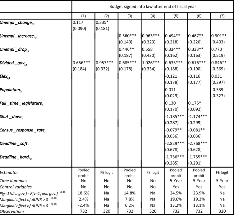
We start out with the simplest of our measures of budget lateness, the binary variablelate_budget. Columns (1) to (4) in Table 2 present results from some basic estimations in which we have only included our two main explanatory variables of interest: The change in the state unemployment rate and a dummy variable for divided government. We use a pooled probit estimator as well as the …xed e¤ect logit estimator.26
In columns (1) and (2) we simply include the change in the unemployment rate, without distinguishing positive changes from negative changes. The change in the unemployment rate and divided control of the government are both associated with more frequent occurrences of late budgets. However, these speci…cations impose a linear e¤ect of changes in the unemploy-ment rate, in the sense that decreases in the unemployunemploy-ment rate are restricted to have the same impact as increases, but with the sign reversed. Columns (3) and (4) relax this restriction by explicitly separating positive changes in the unemployment rate from negative changes. More precisely, the variable unempl_increase is equal to the change in the unemployment rate if the change is positive, and takes the value zero in all other cases. The variable unempl_drop
is equal to theabsolute value of the change in the unemployment rate if the change is negative, and otherwise zero.27 This reveals an important non-linearity: As expected, increases in the unemployment rate are associated with higher probabilities of observing budget delays, relative to a stable unemployment rate. In contrast, a drop in the unemployment rate does not appear to lower the probability of budget delays. If anything, delays are more likely when the state unemployment rate drops below the level from the previous year, as our model would predict.
2 5In general, we wish to include time dummies to capture heterogeneity across time. But since economic conditions are highly correlated across states, it may be di¢ cult to disentangle the e¤ect of national trends from the e¤ect of changes in …scal climates. This means that precise estimation of the coe¢ cients on the unemployment variables may be di¢ cult if we also include yearly time dummies. As a compromise, we therefore use dummies for 5-year periods to capture national trends, rather than yearly dummy variables. Using yearly time dummies yields similar coe¢ cient estimates but with substantially higher standard errors on the cyclical variables.
2 6The Fixed E¤ect logit can only be estimated for the 20 states that have have some variation in the dependent variable (not all 0’s or 1’s).
2 7With these de…nitions, the restriction imposed in columns (1) and (2) is that the coe¢ cient on unempl_increaseis equal to minus one times the coe¢ cient onunempl_drop.
But as the model also predicts, the impact of a drop in the unemployment rate appears to be weaker than the impact of a similar-sized increase: The coe¢ cients on drops in the unemploy-ment rate are always smaller than the coe¢ cients on increases, although the di¤erences are not statistically signi…cant.
To illustrate the magnitude of the e¤ects, we calculate the marginal e¤ects of the explana-tory variables in the probit estimations. Columns (3) suggest that, compared to a zero change, a one percentage-point increase in the state unemployment rate increases the likelihood that the state budget will not be signed into law before the new …scal year by 7.8%-points. The corresponding number for a one percentage-point drop in the unemployment rate is 6.2%-points. Compared to a uni…ed government, divided control of the state government raises the probability of a late budget by 14.8%-points.
<Table 2 about here. [Binary response models, 1988-2007]>
Columns (5) to (7) include a full set of control variables, as described in the previous section. Adding control variables does not change the main results: Divided government signi…cantly increases the probability of a late budget, and so do increases in the unemployment rate. Drops in the unemployment rate also appear to increase the probability of late budgets. The estimated e¤ect is signi…cant on a 5% level when using the pooled probit estimator, but not quite so when we use the …xed e¤ect logit estimator (the p-value is 0:14). The coe¢ cient on unemp_dropis in all cases smaller than the coe¢ cient onunemp_increase, but the di¤erences are again not statistically signi…cant.
Turning to the control variables, we …nd no e¤ect of election years in either of the columns, in contrast to our priors. In column (5) we omit state …xed e¤ects to estimate the e¤ect of a range of time-invariant state characteristics. As expected, we …nd a strongly signi…cant neg-ative impact of deadlines that limit the length of the legislature’s regular session. Somewhat surprisingly, the results suggest that "soft" deadlines have a stronger impact than "hard" dead-lines. At a p-value of 0.12, the di¤erence is borderline statistically signi…cant. Less surprisingly, the coe¢ cient on shut_down shows that late budgets are less common in states where they may result in shutdowns of state government activities.28 Also in line with our expectations is the negative and signi…cant coe¢ cient on census_reponse_rate, which suggests that late budgets are indeed less common in states with a high level of social capital. Our results for super majority requirements (not reported) do not suggest in any way that such requirements
2 8Although in line with our theoretical priors, we would advise caution in interpreting this particular result: Many of those states that list shutdown as a likely (or even unavoidable) outcome of a late budget have never actually experienced a late budget in recent times. While this could of course re‡ect a causal relationship from budget procedures to outcomes, the causality could also run in the opposite direction. States that have never experienced late budgets can "a¤ord" to warn of dire consequences in case of a highly hypothetical budget delay. Experience suggests, however, that once faced with an actual budget stalemate, state governments have a tendency to soften the rhetoric and be innovative in their e¤orts to avoid very harsh consequences.
increase the frequency of late budgets. This is a consistent …nding throughout our empirical analyses.29 Finally, in contrast to our priors, the results in column (5) do not provide any evidence that full-time legislatures are more prone to producing late budgets than part-time legislatures. This could of course re‡ect that there is in fact no causal e¤ect, but it could also be caused by a problem of multicollinearity. In particular, f ull_time_legislature and
population are highly correlated, both individually insigni…cant, but jointly signi…cant at a 10% level (p-value of 0.07). In column (6) we therefore leave out population. This produces the expected positive and signi…cant coe¢ cient on f ull_time_legislature.
5.2 Linear regression models
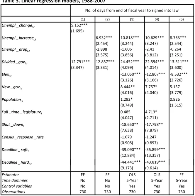
The results in this section exploit the full variation in our measure of budget lateness. This allows us to study the length of budget stalemates, rather than the frequency. As in the previous section, we start out with some parsimonious speci…cations. Columns (1) and (2) in Table 3 report basic …xed e¤ects estimations with the change in the unemployment rate (separated into drops and increases in column (2)) and a dummy for divided government as the only explanatory variables. The results are in line with those from the previous section: Divided government is strongly associated with longer budget negotiations. The change in the unemployment rate, when included in its simplest form, is also positively related to our measures of budget lateness. But as in the previous section, distinguishing positive changes from negative changes suggests that the relationship is non-linear: A rise in the unemployment rate increases the expected length of the budget adoption process, as can be seen from the positive and signi…cant coe¢ cient on unempl_increase. The coe¢ cient on unempl_drop, on the other hand, is imprecisely estimated, and there is no solid evidence that a falling unemployment rate has any impact on the length of budget negotiations. These results suggest that economic slowdowns have a greater impact on the duration of budget negotiations than economic upswings. In terms of magnitude, the estimates indicate that a 1 percentage-point rise in the unemployment rate postpones …nal enactment by about a week.
<Table 3 about here.[Linear regression models, 1988-2007]>
In columns (3) to (5) we include our full set of control variables. This produces even larger coe¢ cients on unempl_increase. The coe¢ cient is signi…cant at the 1% level in all columns. In contrast, the estimated coe¢ cients onunempl_dropare small and statistically insigni…cant across all columns. 30 Divided government again has a large and highly signi…cant e¤ect on the
2 9
We do not elaborate further on this but a full set of estimation results, including estimated coe¢ cients for super majority requirements, can be obtained from the authors upon request.
3 0
Unlike the results in the previous section, the coe¢ cients on unempl_increase and unempl_drop are now signi…cantly di¤erent at a 1% level across all columns. In contrast, the hypothesis that the coe¢ cient
expected length of the budget process. Compared to a uni…ed government, our results show that the expected length of the budget process is about two weeks longer (using the …xed e¤ect estimate) when the state government is under divided control.
Unlike in the previous section, we now …nd a signi…cant e¤ect of election years. As expected, budget negotiations are shorter in election years than in non-election years. The di¤erence is estimated to be between one and two weeks. The …rst budget adoption process under a new governor appears to …nish a little later than in other years. Rookie governors sign the budget about a week later than governors who have led at least one budget negotiation process, although the di¤erence is not statistically signi…cant when state …xed e¤ects are included.
Turning to the time-invariant variables, we again …nd highly signi…cant e¤ects of deadlines that limit the length of the legislative session. State budgets tend to be signed into law 2-3 weeks earlier in states where a delay would trigger a shutdown of non-essential services than in states where such shutdowns cannot happen. There is some evidence that higher social capital is associated with shorter delays, but the results are now not signi…cant. Finally, parallelling the results from the previous section, we …nd a positive but statistically insigni…cant coe¢ cient on f ull_time_leg when we also control for state population size. The coe¢ cient becomes much bigger and statistically signi…cant whenpopulationis excluded, as shown in column (4).
5.3 Censored models
A potential issue with our dependent variabledays_lateis the manner in which negative values are treated. To illustrate, governors usually sign the budget quickly after receiving it from the legislature. Days_late will then record a negative value if this happens before the end of the …scal year. But some governors sometimes choose to postpone signing the budget until the last day of the …scal year for ceremonial reasons only. In such cases, the postponed enactment is not due to a budget stalemate, but days_late records a zero, rather than a negative value. Thus, the variation in days_late that is within the negative domain may just re‡ect unimportant, idiosyncratic noise.
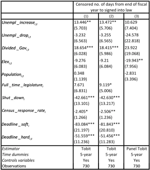
In order to deal with this issue, we left-censor our dependent variables at zero in this section. By censoring the data we can view budget negotiations as a process that either leads to a timely budget or a delay of some (stochastic) duration. Zero or negative values of days_late then indicate a corner solution outcome, while strictly positive observations re‡ect interior solution outcomes. In Table 4 we use the Tobit model as well as the Honore (1992) semi-parametric panel Tobit estimator with …xed e¤ects on the left-censored version, days_late_cens; of our dependent variable.
on unempl_increase is equal to minus one times the coe¢ cient onunempl_drop(the restriction imposed in column (1)) is now only rejected at the 10% level in column (5).
<Table 4 about here. Censored outcomes, 1988-2007>
The results broadly con…rm our previous …ndings. Starting with the Tobit estimates in columns (1) and (2), the estimated e¤ect of an increase in the unemployment rate has the usual positive sign and is signi…cant at a 5% level. As in the linear regressions, the coe¢ cient on unempl_drop is negative, but numerically small and statistically insigni…cant. As usual, the coe¢ cient estimate on divided_gov is positive and highly signi…cant. The results for the time-invariant variables also resemble the results in the previous sections: Legislative session deadlines reduce the expected duration of budget delays, and so do "shut down" provisions and higher levels of social capital, as proxied by the Census response rate. As usual, the coe¢ cient on f ull_time_legislature is positive but insigni…cant when population is included, but it becomes signi…cant at a 10% level when population is omitted, as shown in column (2). The coe¢ cient estimates produced by the Tobit …xed e¤ect estimator in column (3) have the same sign as the Tobit estimates, but they generally lack precision. The p-value forunempl_increase
is 0.15.31
5.4 Fiscal institutions and economic ‡uctuations
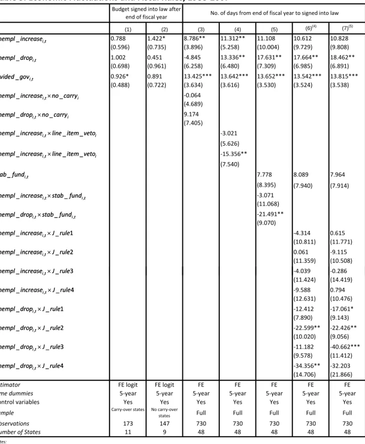
If ‡uctuations in economic activity cause delays in the adoption of state budgets, then we should expect …scal institutions that in‡uence policymakers’ability to smooth such ‡uctuations to a¤ect the relationship between economic conditions and the occurrence of delays. In this section we examine the interaction between two such institutions, balanced budget rules and budget stabillization funds, and the change in the state unemployment rate. Recall the intuition from our model: A change in the amount of available resources relative to the baseline, whether positive or negative, increases the stakes in budget negotiations and produces longer delays. Following this logic, we should expect budget stabilization funds that ease smoothing by forcing extra saving in good years while providing back-up resources in bad years to alleviate the impact of economic ‡uctuations.
The case of balanced rules is slightly more complicated. On the one hand, balanced budget rules may hinder smoothing in bad times and could therefore exacerbate the e¤ect of …scal deteriorations. On the other hand, strict rules may promote …scal discipline in good years and therefore dampen the e¤ect of rising revenues. All states except Vermont have some kind of balanced budget requirement, but the strictness of these requirements varies considerably. Below we consider two variables that have been used in the literature to characterize the
3 1The estimated coe¢ cient on divided_gov is insigni…cant in column (3). However, if we distinguish splitbranch governments from splitlegislature governments an issue that we address further in the next section -we …nd a signi…cant e¤ect of split legislatures, and a considerably smaller and statistically insigni…cant e¤ect of split-branch governments.