On Threshold-Free Error Detection for Industrial Wireless Sensor Networks

(1)

Cleveland State University

EngagedScholarship@CSU

Electrical Engineering & Computer Science

Faculty Publications

Electrical Engineering & Computer Science

Department

5-2018

On Threshold-Free Error Detection for Industrial Wireless Sensor

Networks

Jianliang Gao

Central South University

Jianxin Wang

Ping Zhong

Haodong Wang

Cleveland State University, [email protected]

Follow this and additional works at: https://engagedscholarship.csuohio.edu/enece_facpub

Part of the Digital Communications and Networking Commons, and the Electrical and Computer Engineering Commons

How does access to this work benefit you? Let us know!

Repository Citation

Gao, Jianliang; Wang, Jianxin; Zhong, Ping; and Wang, Haodong, "On Threshold-Free Error Detection for Industrial Wireless Sensor Networks" (2018). Electrical Engineering & Computer Science Faculty Publications. 448.

https://engagedscholarship.csuohio.edu/enece_facpub/448

This Article is brought to you for free and open access by the Electrical Engineering & Computer Science Department at EngagedScholarship@CSU. It has been accepted for inclusion in Electrical Engineering & Computer Science Faculty Publications by an authorized administrator of EngagedScholarship@CSU. For more information, please contact [email protected].

(2)

On Threshold-Free Error Detection for Industrial

Wireless Sensor Networks

Jianliang Gao

, Member, IEEE,

Jianxin Wang,

Senior Member, IEEE,

Ping Zhong ,

and Haodong Wang

I. Introduction

NDUSTRIAL wireless sensor networks (IWSNs) are widely adopted to monitor real environments as a promising paradigm for industrial automation [1]. In IWSNs, a large number of sensor nodes are deployed to measure the physical parameters of the surroundings, monitor the machine status, and transmit the readings (sensed data) to the remote control center [2], [18]. Based on the collected data, the control center can make decisions and send commands to machinery actuators and

trigger necessary actions. However, erroneous readings could generate strong side effects on the subsequent control chain, leading to wrong decisions and inappropriate control actions. The accuracy of the sensor readings is therefore considerately crucial, e.g., in smart cities [3], Internet of Things [4], railway monitoring systems [5], or social networks [6]. In safety critical applications such as the radiation monitoring system deployed after the emergency at Japanese Fukushima Dai-ichi nuclear plant in 2011 [7], sensor errors could result in damage to industrial devices and environment, or in the worst case scenario, result in loss of life [8].

One of the major sources for big data is the datasets collected by IWSNs. It has potential of significantly enhancing people’s ability to monitor and interact with their environment. However, sensor errors are unavoidable in many industrial monitoring systems [9]. The causes for sensor errors mainly consist of the following situations.

1) The damage by the harsh industrial environment. Sen- sor nodes are expected to operate autonomously and they are directly exposed to a harsh and uncontrolled environment. Therefore, sensor nodes might be contaminated and damaged by the harsh industrial environment [10]. 2) The security breach. An attacker might capture some sen-

sor nodes and inject hostile codes. The captured nodes might report erroneous readings according to the attacker’s instructions [11].

3) The aging phenomenon. This could induce the descent of the measurement precision as the passing of time. For example, the sensor might become biased and suffers a gradual offset value independent of its monitoring environment [12].

The common feature of erroneous readings is that they fail to accurately reflect the industrial monitoring environment and might cause serious consequences. An error detection system, therefore, plays an important role in IWSNs. Since spatiotem- poral correlations exist among sensor readings, some existing solutions obtain the estimated values of sensor nodes by exploiting the spatial [13] and temporal correlation among sensor readings [14]. They then identify the erroneous readings by comparing the sensor readings to the estimated values. Instead of comparing readings, some other approaches check the model consistence between sensors. For newly arrived readings, the co efficients of the linear model are trained again and are compared to the previous coefficients. If the differences exceed a given threshold, the new arriving readings are classified as errors [15].

(3)

Traditional error detection approaches all require thresholds to judge the states of sensor data. Unfortunately, it is difficult, if not impossible, to obtain a proper threshold in real-world ap plications. If the threshold is too high, many errors may hide in the normal readings without being identified, which will cause low detection accuracy. On the other hand, many normal read ings could be diagnosed as errors if the threshold is too low, which causes high false alarm rate. Threshold-based technique is therefore hard to determine a special threshold for various unpredictable errors. A good error detection method should be accurate in identifying an error with a low false alarm rate.

In this paper, we propose a threshold-free error detection (TED) approach, which is a novel error detection approach with-out requiring a threshold to judge a reading normal or erroneous. By exploiting the information related to the spatial and temporal relationships among sensor data streams, we first construct a correlation graph where vertexes are the sensors and links are associated with the sensor-to-sensor pairwise relationship. For each sensor pair, the estimated value via the linear model is compared to the measured value. In particular, the residual between them is mapped into a high-dimensional feature space. The final diagnosis of node state is executed on a base station (BS) using the correlation graph with the link states labeled. This paper focuses on the error detection and takes the assumption that time synchronization [16], [28] and reliable real-time transmission [17]—[19] have been achieved. Specifically, the main contributions of this paper are summarized as follows.

1) We study error detection in the context of IWSNs. We first propose a threshold-free approach to detect errors in sensor data.

2) We design efficient models that reveal the temporal and spacial correlations in sensor networks. In particular, we map residual data into a high-dimensional feature space, which efficiently classifies the input residuals without requiring any threshold.

3) We propose a two-stage error detection approach, which achieves accurate detection results. Especially, it elim inates the influence of the bias caused by noises and models, and accordingly leads to more accurate diagno sis results.

4) We evaluate the performance of error detection on real datasets and extensive simulations. The results show that the TED approach detects the errors accurately with low false alarm rates.

The rest of this paper is organized as follows. Section II presents the correlation graph construction stage of the TED approach. Section III presents the error diagnosis stage of the TED approach. Experimental results are given in Section IV. Section V surveys the related works. Discussions are presented in Section VI. Conclusions are drawn in Section VII.

II. Constructing Correlation Graph

The TED approach consists of two stages. In the first stage, the correlation graph is constructed based on the trained models between sensor pairs. In the second stage, reading errors are diagnosed by utilizing the correlation graph. In this section, we propose a correlation graph to characterize the correlation

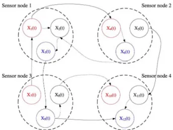
Fig. 1. Illustration of networked sensor data.

among the networked sensor data streams. Fig. 1 illustrates an example of correlation among four sensor nodes. Each sensor node in Fig. 1 has three different sensors such as humidity sensor, temperature sensor, and so on, which are distinguished with different colors. For example, three kinds of sensor data streams of sensor node 1 are denoted as X1 (t), X2(t), and X3(t), where t is the sample time. The correlation between the same kind of sensors are linked with solid line, e.g., the link between X1(t) and X4(t); and others are linked with dash line, e.g., the link between X1(t) and X2(t). As a preliminary foundation, it is crucial to construct the relationship quantitatively between sensor pairs.

A. Modeling the Relationship Between Sensor Pairs Since sensor responses depend on the common physical sys tem, a linear relationship exists between the system outputs measured by the sensors [22]. In our approach, two sensor data streams measured by sensor i and sensor j are denoted as Xi and Xj, respectively, which can be viewed on different physical measurements (e.g., temperature and humidity). The pairwise relationship between Xi and Xj is formulated as following using AutoRegressive model with eXogenous input (ARX):

A(z)Xi(t) = B(z)Xj(t - k)+εij(t) (1) where z is the backward time-shift operator and k is the input- output delay; t is the time variable and (f) are independent and identically distributed random variables accounting for the noise; and A(z), B(z) represent the z-transform functions of model parameters and are presented as follows:

A(z) = 1 + a1z-1+ ... +amz-m

B(z) = bl+b2z 1 + --- + bnz -n+1. (2) According to (1) and (2), the ARX model can be further expressed as follows:

Xi(t) + a1Xi (t — 1) + ■ ■ ■ + am Xi(t —m) = b1Xj(t — k)

+ b2Xj (t — k — 1) + ...+ bnXj (t — k — n+ 1) + εij (t) (3)

(4)

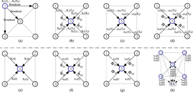
Fig. 2. Schematic diagrams of the proposed approach. (a)-(d) show the first stage. The ARX model parameters are trained by the training sequence pair t = 1,... .T0 [see (a) and (b)]; the OCSVM models are trained by the residuals eij (t), and thereby obtain the decision function ϕij [see (c) and (d)]. (e)-(h) show the second stage. The states of links sij(t) are quantized using the trained models with X(t),eij[see (e)-(g)]. Finally, in (h), the link states s(t) are transmitted to the BS for further diagnosis. (a) Broadcast training data. (b) Train ARX parameter. (c) Compute residuals. (d) Train OCSVM model. (e) Overhear current readings. (f) Compute residuals. (g) Estimate link states. (h) Iterative diagnose on BS.

where m controls the extent of autocorrelation in Xi(t), nde- termines the number of previous samples of Xj(t) affecting the current value Xi(t). and kis the corresponding delay. The coefficient parameter ϴ can be defined as follows:

ϴij =[a1,...,am,b1,...,bn]T

.

(4) 6. Constructing Correlation Graph

In order to construct the correlation graph, the coefficient parameters ϴijof sensor pair should be obtained first. From (3) and (4). it can be drawn that

xi(t) = [-MX]-^+sv(i) (5) where A', = [A,(f — I). A',(f — 2)...X,(t — z»)].and X, =

PQ(i-*+l)...tj(t-k-(n - 1))].

At the beginning of the system deployment, the sensor net work. data are collected for training ARX model, i.e., getting the parameters Given the collected training data [X, (t). A",. A"j

in (5)]. the training process is obtained as follows [26]:

(6)

where X,(t|0o) = AJ • I < t < To.

In this way, we construct the relationship between pair sen sors. Then, a correlation graph representing the sensor network can be formulated as follows:

(7) where V is the set of the sensor readings A; (f), and E is the set of links between v, v ϵV. Sv, Se are the state sets of the vertices and links, respectively. At sample time t. if the relationship

of two sensor readings (Xi (t), Xj(t)) violates the trained relationship, sij (t) ϵSe is set to “1,” otherwise “0” is set. Similarly, if a vertex state in correlation graph is set to “1,” it means the corresponding sensor reading is diagnosed as error. Therefore, we first detect link state set Se; and based on Se, we further determine vertex states 5„, which indicate the current reading of the corresponding sensor is error or not.

Fig. 2(a) and (b) shows an example of the above-mentioned process. In a graph G, every vertex i broadcasts its readings Xi(t), t = I...T0.Taking vertex 1 in Fig. 2(a) as an example, it broadcasts the readings X1 (t), t = 1,..., T0, to its neighbor vertices 2, 4, and 5. As shown in Fig. 2(b), vertex 5 receives X1(t), X2(t), X3(t), and X4(t) , t= 1,... ,T0, from its four neighbor vertices. The ARX model parameters (ϴ51, ϴ52 and ϴ53, 6*54) are then trained according to (6).

C. Model to Determine Link States

After getting the trained parameter ϴij= [a1,... ,am, b1,..., bn]T, the estimated value of sensor i can be obtained as follows with given ϴij and Xi, Xj:

m Xij (t) = J? -am'Xi (f - m') m'= 1 (8) n + ' bniXj{t -k — n!-\-Y). n'= 1

The next step is to determine whether the residuals between estimated values and measured readings are correct. For example, sensor i can obtain an estimated value under parameters The residual between the current reading Xi(t) and the estimated value Xij(t) is then calculated by the following

(5)

equation:

(9) With e(t). t = 1...T0, as training samples, we model the problem of link status as one-class support vector machine (OCSVM);

(10)

where T0 is the number of training samples, vis an upper bound on the fraction of training samples lying on the wrong side of the hyper plane, and k(e(t),e(t')) is the kernel function. We adopt radial basis function kernel, which is defined as follows:

(11) where σ is a free parameter and its value can be selected by the method in [20]. The optimal solution α is obtained by training set as which should all be classified as "correct” class. Then, the OCSVM decision function Φ(e) can further be given as follows:

To

Φ(e) = (12)

t=l

where w = (■, ■) is the inner product opera-tor, and φ(.) is a map function from the input space to a feature space. In the OCSVM, the mapping function satisfies <^(e(t)),^(e(t'))) = exp(-l|e(t)2~f2!'}I1 ). If $(e) > 0, then e

is labeled “normal”; otherwise it is labeled “faulty.”

In practical applications, collecting samples of faulty system states can rather be expensive. On the other hand, simulations cannot guarantee that all the faulty states are included. In our approach, only positive samples are required to train the OCSVM model.

Fig. 2(c) and (d) demonstrates the training procedure of OCSVM model. Taking node 5 as an example, residuals e5j (f), (j = 1,..., 4, t = 1,..., T0), are taken as the training inputs for the OCSVM model, and the model decision functions (Φ51, Φ52, Φ53, and Φ54) are then obtained, respectively.

III. Error Diagnosis: Two-Layer Mechanism The error diagnosis stage of the TED approach includes two layer processing: The sensor node layer and the BS layer. In the sensor node layer, sensor node collects neighbor readings to calculate the estimated values and the corresponding residuals. Each node will then output the judgment about its residuals, i.e., the link states of the correlation graph. In BS layer, BS diagnoses each node state iteratively according to the link states in the correlation graph.

Algorithm I: Diagnosis for Link Slates of the Correlation Graph.

Input: Sensor reading sequences Xi(t) and Xj(t),

Output: The link states sij(t) between Xi and Xj,

sij(t) ϵSe.

1: Train ARX model coefficient ϴjj according to (6): 2: for each Xi(t) and Xj(t), 1 ≤t ≤ T0 do 3: Compute X,j (t)using (8);

4: Compute residuals eij (t) using (9); 5: end for

6: Train OCSVM model based on the residual values

eij(t);

7: t = To; 8: repeat

(6)

residuals , (t) are classified by the OCSVM model described in the previous section, and link states sij(t) ϵ Se are obtained according to (13). Finally, as shown in Fig. 2(h), the link states are reported to the BS for further diagnosis of vertex states. B. Diagnosis for Vertex States

After receiving all link states from the sensor node layer, the BS has a view of the correlation graph for sensor network. Further diagnosis is carried out on the BS to determine the vertex state in the correlation graph, which indicates whether a sensor reading is erroneous. In this section, we propose an iterative method to diagnose the vertex states.

The basic idea is to calculate the vertex states iteratively ac cording to the link states and the neighbor vertex states. Given a link state, there are four probabilities corresponding to a pair of sensor state P(si|sJ, s.t, s3 = 0,1). The state transition matrix is = P(si\s3), where si, sj ϵ{0,1}. Since the proba-bility P is related to the state of the link, the transition matrix M(i, j) can be detailed as follows:

if the link state is “0” (14) if the link state is “1”

where β0, β1 are the transition factors when the link state is “0”. means the probability that vertex state is “0” on condition that its neighbor state is “0” when link state is “0”. β0means the probability that vertex state is “1” on condition that its neighbor is “1” when link state is “0”. are the transition factors when the link state is “1”. (1 - β'0) means the probability that vertex state is “0” on condition that its neighbor state is “0” when link state is “1”. (1 - β'1) means the probability that vertex state is “1” on condition that its neighbor is “1” when link state is “1”.

In order to measure the trend of a vertex state of “0” or “1,” we introduce the self-confidence function for any sensor i:

(15)

where N0,i is the number of sensor i s neighbors whose readings are classified as correct, and Ni is the total number of sensor i s neighbors. The elements vi,(0),vi(1) are the self-confidence values for state “O’ and “1,” respectively.

The probability of vertex state is calculated as follows: N

P(st = 0 = ^i(C)x n M(sQi(k),<), C G {0,1} (16) k=l

where is the state of sensor j; ( is the possible state value ( G {0,1} (0: correct; 1: faulty), and Q,(k) is the kth neighbor of sensor i. The vertex state is then updated as the higher probability:

Si = arg max P(si = ς). (17) fefo.i}

Algorithm 2: Diagnosis for Vertex States of the Correlation Graph.

Input: Correlation graph with link states G(V, E,Se). Output: Each vertex i's state si, si ϵ Sv.

1: for each vertex i, i ϵ V. do

2: Calculate its self-confidence value v according to (15);

3: Initialize node state si = arg max fe{0.1} 4: end for

5: repeat

6: tag = 0;

7: for each vertex i, i ϵ V, do

8: Compute probability of each state using (16); 9: Determine new state s' according to (17); 10: if Sj / s'i do 11: Si = s'; 12: tag = 1; 13: end if 14: end for 15: until (tag = 0);

If a vertex’s state changes, other vertices’ states update iteratively until the states become stable. Algorithm 2 shows the diagnosis detail on a BS. Lines 1-4 demonstrate the initialization for each vertex of correlation graph, where the initial state (“0” or “1”) is determined by the maximum self-confidence as shown in Line 3. Lines 5-15 are the iterative diagnosis procedure. In an iteration, new states are obtained according to (17) and the iteration terminates if there is no state update.

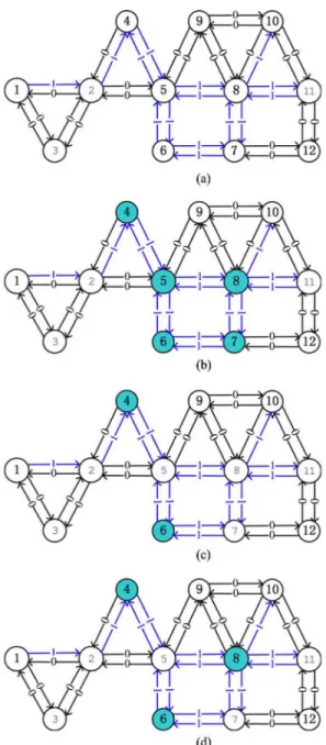
Example: Fig. 3 shows an example of the iterative diagnosis. Fig. 3(a) is the correlation graph of a sensor network. There is a direct link from vertex j to vertex i [in Fig. 3(a)] if vertex j is used to estimate vertex i. The number (“0” or “1”) on a link denotes the state of the link, which is the output of distributed link states diagnosis. The transition matrix parameters are set as β0 = = 0.8 and β = (3[ =0.5. According to Algorithm 2 (Lines 1-3), vertices 4, 5, 6, 7, and 8 are set faulty, as shown in Fig. 3(b). In the first iteration, vertices 5, 7, and 8 change their states, as shown in Fig. 3(c). Taking vertex 8 as an example, P(s8 = 0) = 0.4 x 0.5 x 0.5 x 0.8 x 0.8 x 0.2 and

P(s8 = 1) = 0.6 x 0.5 x 0.5 x 0.2 x 0.2 x 0.8, and P(s$ = 0) > P(s8 = 1). Thus, vertex 8 is set as “0” after the first iteration. It is interesting that vertex 8 changes back to “1” because P(s8 = 1) > P(s8 = 0) in the second iteration. After two iterations, the states of vertices become stable. Therefore, in Fig. 3(d), the states of the vertices are the final diagnosis results for current readings. The readings of vertices 4, 6, and 8 are diagnosed as errors in this example.

IV. Experimentsand Results

To verify the effectiveness of our approach for detecting er rors in sensor data stream, experiments are conducted with both real-world datasets and simulation datasets. There are two

(7)

pur-Fig. 3. Example of iterative diagnosis on a BS. Vertices 4, 6, 8 are diagnosed as faulty in the end. (a) Correlation graph with link states. (b) Initiate the sensor states. (c) First iterative result. (d) Second iterative result (stable).

poses for these experiments: 1) Demonstrate the significant benefit in terms of detecting errors of a pair of sensor data streams (see Section IV-A); 2) demonstrate the effectiveness (detection accuracy and false alarm rate) of our approach on a simulated wireless sensor network (see Section IV-B).

A. Detection Errors for Sensor Pairs

We demonstrate the effectiveness using two real-world datasets. One is a pair of temperature and humidity sensor readings, which we sampled from February 1, 2015 to February 20, 2015. The other comes from a monitoring system for rock

fall forecasting [15]. A hidden Markov model (HMM) based method [15] was used to detect errors from a pair of sensor data streams and we compare the effectiveness of our approach with them.

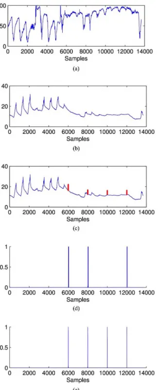
1) Dataset of Temperature and Humidity Monitoring System: We deployed a pair of sensor nodes to sample surrounding thermal and humidity at the same time. The data streams and the detection results are shown in Fig. 4, where the horizontal axis denotes the sample number and vertical axis denotes the detected values accordingly. Fig. 4(a) and (b) shows the original humidity and temperature data streams. There are 13 669 samples used in this experiment and the first 6000 samples are chosen to train the model. To verify the capability of fault detection, we artifi- cially inserted four errors into the original temperature samples at sample 6001, 8001,10001, and 12 001, as shown in Fig. 4(c).

The four erroneous values are amplified 1.35 x to their original values, respectively.

Fig. 4(d) and (e) shows the detection results of the HMM- based method and our TED approach, respectively, where each sample is denoted as “1” or “0” when an alarm is reported or not. As can be seen in Fig. 4(d) and (e) that HMM-based method has failed to detect the third error at sample 10 001, whereas TED detects all the four errors correctly. Another weakness of HMM- based method is that it causes more false alarms. For example, it raises 39 alarms to the error at sample 6001, whereas our method only raises four alarms. Furthermore, the false alarms can be eliminated in the second stage of error detection of TED at the BS.

2) Dataset of Rock Fall Forecasting System: The dataset of the readings for rock fall detection consists of the measurements coming from a new generation of intelligent clinometer sensors [15]. We consider the temperature and clinometer measurements recorded from August 1, 2011 to October 31, 2011. The dataset is composed of 2844 samples, and the first 1500 samples are chosen as the training sequence.

Fig. 5 presents the data and detection results. Fig. 5(a) and (b)

shows the original clinometer and temperature measurements.

Fig. 5(c) shows the modified temperature data after inserting three errors at sample 1501, 2001, and 2501. These errors are offset errors with an average offset of 3 and additional noise N(0,0.32). Fig. 5(d) and (e) shows the detection results of the HMM-based approach and the TED approach, respectively. As can be seen that the inserted three errors are all detected by HMM-based approach and TED. However, it can be further observed that our TED approach has at least two advantages over the HMM-based approach: TED has less false alarms and shorter delay of the detection to the errors. For example, for the error at sample 1512, the numbers of alarms are three and 77 with our TED approach and the HMM-based method, respectively. HMM-based method takes 11 samples to detect the error inserted at sample 1501, whereas TED is able to detect this error with only one sample delay. It demonstrates that TED can detect the errors more accurately and with less delay. Another phenomenon occurred in the experiment is that several alarms are reported near sample 2400, which is difficult to judge whether it is a true error or false alarm. Fortunately, this can be further diagnosed in the second stage of TED.

(8)

Samples

(e)

Fig. 4. Error detection on a pair of humidity sensor and thermal sensor. (a) Original humidity sensor data. (b) Original temperature sensor data. (c) Temperature sensor data with four artificial errors. (d) Detection results of HMM-based method. (e) Detection results of the proposed TED approach.

B. Simulation Experiments of a Wireless Sensor Network

In this section, we conduct experiments on a simulated wireless sensor network (WSN) to further verify the detection effectiveness. The effectiveness is evaluated by two metrics: detection

Samples (d) 1 r 0.5

-ol

---

X---X--- --- ---LJ---, 0 500 1000 1500 2000 2500 3000 Samples (e)

Fig. 5. Error detection on a rock collapse monitoring system. (a) Original clinometer sensor data. (b) Original temperature sensor data. (c) Temperature sensor data with three artificial errors. (d) Detection results of HMM-based method. (e) Detection results of the proposed TED approach.

accuracy and false alarm rate. Detection accuracy is the ratio be tween number of erroneous readings detected as erroneous and the total number of erroneous readings present in the network. False alarm rate is defined as the ratio of the number of error free readings detected as erroneous to the total number of error free readings.

(9)

TABLE I

Parameter Settingsin Simulations

Parameters Values

Number of sensor nodes 400 Deployment area 20 x 20 (units) Communication radius 1.2, 1.5 (units)

Length of samples 700

Length of training samples 600 Length of validation samples too Error gain coefficient (γ) 10%, 50% Error rates 0.05.0.1.0.15. 0.2.0.25

Table I shows the major parameter setting of the simulation experiments. We simulate a WSN with 400 sensor nodes that are evenly deployed in a 20 x 20 (units) area. A signal source lies in the center of this area, which generates signal according to ξ(t) = 80 sin (0.5t). The data stream x(t) is then measured by sensors in the WSN as follows:

<(*) ,

xit) = —, --- h eft)

(\/(2V -

7.-J2 +

{.Py ~ qy)-

+

1 )

d

where (px,py) and (qx,qy) are the coordinates of the sensor node and the signal source, respectively. d is the signal de- cay exponent [27]. ϵ(t) ~ N(0,0.012) is a zero-mean Gaussian noise, which reflects the real exogenous input.

In the simulations, the first 600 samples are used as training samples, and the following 100 samples, with some of them randomly set as erroneous. Denoting the generated data without error as vn, the data with gain error can be

v'n = vn + γ X W (18)

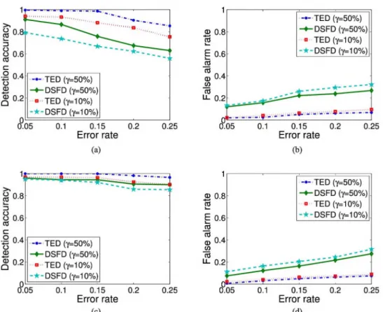
where γis gain coefficient and v'n is the readings after inserting artificial errors in the simulations. In theory, the more the reading deviates from the correct value, the easier it is to be detected. In this experiment, two different gain coefficients (7 = 50% and 7 = 10%) are tested. Another variable parameter is the average number of neighbors. By setting communication radius as 1.2 and 1.5 units as shown in Table I, two kinds of neighbor numbers (N = 4 and N = 8, respectively) are simulated to validate the effect of spatial correlation.

Fig. 6 shows the detection results for various error rates from 0.05 to 0.25. The results are compared with distributed self-fault diagnosis (DSFD) method [14]. The DSFD algorithm consists of two phases: initialization phase and self-diagnosis phase. In the first phase, each sensor node transmits its sensing readings to neighboring nodes. In self-diagnosis phase, a sensor node computes the median value of its neighbor sensor readings. Then, the median values are compared with the current readings. Finally, the fault state is obtained by comparing the residuals between them with a given threshold. The reasons to compare with DSFD are as follows.

1) The problems to deal with are the same. Both our TED method and the DSFD method are focused on solving the error reading detection.

2) Similar to our proposed method, DSFD method is also a distributed method without requiring central powerful nodes.

3) DSFD outperforms the traditional error detection methods such as majority voting method, weighted average method, and weighted median comparison method, as shown in [14].

It can be seen from Fig. 6(a) and (c) that the detection ac curacies of our approach are always higher than that of DSFD method [14] under the same parameters. On the whole, larger number of neighbors can improve the detection accuracy. For example, all detection accuracies are above 0.8 in Fig. 6(c), es pecially for our approach when 7 = 10%. It is because more neighbors mean that more spacial correlations can be utilized. From Fig. 6(b) and (d), it can be seen that our approach achieves much lower false alarm rate compared to DSFD method. It is because, even if there exist some deviations of linear model, the iterative diagnosis of our approach can correct them. But it is difficult for threshold-based methods to achieve high detection accuracy and low false alarm rate simultaneously.

In the proposed scheme, we use OCSVM to model the relationship between sensor pairs. In order to train the OCSVM, a part of sensor samples are adopted as training samples. In the above three studied cases, different amounts of data samples were used for training the proposed models. The motiva- tion of the choice of the numbers is to test the wide ranges of the model parameters. In the two real-world experiments (temperature/humidity monitoring system and rock fall forecasting system), the numbers of training packets are 6000 and 1500, respectively, which consist of less than and more than 50% of the total packets (6000/13669 and 1500/2844). Larger number of training samples increases the time cost. Fortunately, WSNs only need to conduct the model training once during the deployment phase.

V. Related Works

Data errors is a serious problem in sensor-based industrial systems. Wrong sensor data could cause damages if they are not identified. Previous works on error detection of sensor readings are mainly formed by two groups: error detection with reading comparison or with model comparison.

A. Error Detection With Reading Comparison

Error detection with reading comparison utilize the spatial and/or temporal correlations in sensor networks.

To detect errors in structural health monitoring, Liu et al. propose a threshold-based scheme, which utilizes the spacial correlations between sensor readings, to find out faulty readings [21]. Some proposals use statistic features to improve the detection accuracy. For example, median value is used in WMFDS [23]. In these approaches, each sensor node first obtains a statistic value according to its neighbors’s readings and compares it with local measurements. If the differences exceed a given threshold, it is detected as erroneous readings.

To characterize the spacial correlations between neighboring sensors, the study in [24] introduces hidden Markov random

(10)

Fig. 6. Comparative results with various neighbor numbers (N = 4,8) and error gain coefficients (7 = 10%, 50%). (a) Detection accuracy (N= 4). (b) False alarm (N = 4). (c) Detection accuracy (N = 8). (d) False alarm (N = 8).

field (HMRF) model. Using the HMRF model, a sensor node can obtain estimated values from its one-hop neighbors, and the differences between the estimated values and the readings are calculated. With majority voting scheme, if majority differences exceed a given threshold, the current readings are regarded as erroneous. Recently, a DSFD is proposed [14], which also re- quires a given threshold to detect the reading errors.

It can be seen that traditional error detection techniques rely on threshold-based method. The proposed TED approach in this paper addresses this issue by utilizing the inherent features of spatial and temporal correlation to realize accurate error de tection without any threshold. Compared to the previous sen sor error detection approaches, threshold-free approach is more suitable for various real-world industrial applications.

B. Error Detection With Model Comparison

Different from comparison between sensor readings, some researches use new relationship models to detect errors. Alippi et al. propose a data error detection system [15] where they constructed a linear model between a pair of sensors. When data newly arrives, the parameter of linear model is estimated repeat- edly using the newest data belonging to the nearest time window. The estimated parameter value along with previous parameter values are then added to an HMM to calculate a log-likelihood value. Finally, the log-likelihood value is compared with a given threshold to judge whether the newly arrived data are erroneous. A novel method named FIND [25] considers a node faulty if its readings violates the distance monotonicity significantly, which is measured by the received signal strength. Then, the sorted sequence is compared to precalculated sequences to judge which node is faulty. Recently, another efficient scheme named SFDIA is proposed in [8], which can detect the sensor failures in an air- craft system. They combine the sensor readings and the sensor model in a threshold logic. In this way, faulty sensor reading can be replaced with a reliable estimate.

VI. Discussion

Industrial environments are often characterized by complex factors such as fading and shadowing, presence of highly re flective surfaces and interference, which all affect the quality of communication. Some discussions are first presented for the scenario of unreliable communication links and losses of some sensor data. Moreover, industrial sensors typically work in duty cycles, and listening to the neighboring nodes leads to additional energy consumption. Therefore, discussions about tradeoff be tween energy consumption and better error detection are also added in the following.

1) A discussion about possible consequences of unreliable communication links and losses of some sensor data. The proposed TED method includes two stages: training stage and diagnosis stage. At the training stage, both ARX model and OCSVM are trained to characterize the relationship between the readings of sensor pairs. As described in Section I, this paper assumes that reliable real-time transmission [17]—[19] has been achieved. But unreliable communication links and losses of some

(11)

sensor data may affect the error detection. In the training stage, the accuracy of the model may be affected accord ing to (6) if some data is missing. To reduce the neg ative affection, periodic update of training models can improve the accuracy of the model parameters. On the other hand, missing data can be estimated using previous trained model parameters according to (8). In diagnosis stage, the proposed method can tolerate missing sensor data. As shown in (16), the probability of a vertex state is related to its multiple neighboring sensor readings. If only part of the data is missing, the probability can still be calculated by using the other neighbor sensor readings. 2) A discussion about tradeoff between energy consumption

and better error detection.

In low duty-cycle WSNs, it may generate high energy consumption to transmit sensor data. There are some ways to solve this problem.

a) It is not necessary to collect all neighbor read ings for a vertex. In Section IV-B, a simulation comparison about the affection of neighbor num ber is shown in Fig. 6, the detection accuracy has been high when each sensor receives only four neighbor sensors readings (N = 4) although more neighbor sensors readings can improve the accuracy (N = 8). The reason is that the iterative diagnosis stage of the proposed TED method can tolerate some deviations.

b) Sensor node can overhear neighbor sensor readings when they send the readings to a BS.

c) Only the faulty link states are needed to transmit for diagnosis on a BS.

VII. Conclusion

In this paper we proposed TED, a TED approach for sensor-based monitoring systems. Without relying on any given threshold, TED detects errors based on the temporal and spacial correlation. Given readings sequences from sensors, we first design and construct the correlation graph that represents the de- pendence relationship between pairwise sensors. Then, we map the pairwise residuals of the readings into a high-dimensional feature space. Based on the states of the links, an iterative algorithm is developed to finally diagnose the vertex states, i.e., whether a reading is an error. In the whole process, we avoid any threshold to judge the readings. With the extensive simulations and real-world experiments, we demonstrate TED achieves both low false alarm rate and high detection accuracy simultaneously.

References

[1] Z. Iqbal, K. Kim, and H. Lee, “A cooperative wireless sensor network for indoor industrial monitoring,” IEEE Trans. Ind. Informat., vol. 13, no. 2, pp. 482-491, Apr. 2017.

[2] F. Dobslaw, T. Zhang, and M. Gidlund, “End-to-end reliability-aware scheduling for wireless sensor networks,” IEEE Trans. Ind. Informat.,

vol. 12, no. 2, pp. 758-767, Apr. 2016.

[3] A. Alvi, S. Bouk, S. Ahmed, M. Yaqub, M. Sarkar, and H. Song, “BEST- MAC: Bitmap-assisted efficient and scalable TDMA-based WSN MAC protocol for smart cities,” IEEE Access, vol. 4, pp. 312-322, 2016.

[4] X. Liu, S. Zhao, A. Liu, N. Xiong, and A. V. Vasilakos, “Knowledge- aware proactive nodes selection approach for energy management in internet of things,” Future Gener. Comput. Syst., pp. 1-15, 2017, doi:

10.1016/j.future.2017.07.022.

[5] V. J. Hodge, S. Keefe, M. Weeks, and A. Moulds, “Wireless sensor networks for condition monitoring in the railway industry: A survey,” IEEE Trans. Intell. Transp. Syst., vol. 16, no. 3, pp. 1088-1106, Jun. 2015. [6] J. Gao, J. Wang, J. He, and F. Yan, “Against signed graph deanonymization

attacks on social networks,” Int. J. Parallel Program., pp. 1-15, 2017, doi:

10.1007/s 10766-017-0546-6.

[7] E. Ackerman and E. Guizzo, “5 Technologies that will shape the web,”

IEEE Spectr., vol. 48, no. 6, pp. 40-45, Jun. 2011.

[8] S. Hussain, M. Mokhtar, and J. Howe, “Sensor failure detection, identifica- tion, and accommodation using fully connected cascade neural network,”

IEEE Trans. Ind. Electron., vol. 62, no. 3, pp. 1683-1692, Mar. 2015. [9] C. Yang, C. Liu, X. Zhang, S. Nepal, and J. Chen, “A time efficient

approach for detecting errors in big sensor data on cloud,” IEEE Trans. Parallel Distrib. Syst., vol. 26, no. 2, pp. 329-339, Feb. 2015.

[10] P. Tang and T. Chow, “Wireless sensor-networks conditions monitoring and fault diagnosis using neighborhood hidden conditional random field,”

IEEE Trans. Ind. Informat., vol. 12, no. 3, pp. 933-940, Jun. 2016. [11] F. Gandino, B. Montrucchio, and M. Rebaudengo, “Key management

for static wireless sensor networks with node adding,” IEEE Trans. Ind. Informat., vol. 10, no. 2, pp. 1133-1143, May 2014.

[12] G. Re, F. Milazzo, and M. Ortolani, “A distibuted bayesian approach to fault detection in sensor networks,” in Proc. IEEE Globecom, 2012, pp. 634—639.

[13] L. Pan, H. Gao, H. Gao, and Y. Liu, “A spatial correlation based adaptive missing data estimation algorithm in wireless sensor networks,” Int. J. Wireless Inf Netw., vol. 21, pp. 280-289, 2014.

[14] M. Panda and P M. Khilar, “Distributed self fault diagnosis algorithm for large scale wireless sensor networks using modified three sigma edit test,”

Ad Hoc Netw., vol.25,pp. 170-184,2015.

[15] C. Alippi, S. Ntalampiras, and M. Roveri, “A cognitive fault diagnosis system for distributed sensor networks,” IEEE Trans. Neural Netw. Learn. Syst., vol. 24, no. 8, pp. 1213-1226, Aug. 2013.

[16] P. Carbone et al., “Low complexity UWB radios for precise wireless sensor network synchronization,” IEEE Trans. Instrum. Meas., vol. 62, no. 9, pp. 2538-2548, Sep. 2013.

[17] D. Yang et al., “Assignment of segmented slots enabling reliable real- time transmission in industrial wireless sensor networks,” IEEE Trans. Ind. Electron., vol. 62, no. 6, pp. 3966-3977, Jun. 2015.

[18] A. Saifullah, Y.Xu, C. Lu, and Y. Chen, “End-to-end communication delay analysis in industrial wireless networks,” IEEE Trans. Comput., vol. 64, no. 5,pp. 1361-1374, May 2015.

[19] S. Han, S. Zhao, Q. Li, C. Ju, and W. Zhou, “PPM-HDA: Privacy- preserving and multifunctional health data aggregation with fault toler- ance,” IEEE Trans. Inf. Forensics Security, vol. 11, no. 9, pp. 1940-1955, Sep. 2016.

[20] Y. Xiao, H. Wang, and W. Xu, “Parameter selection of Gaussian kernel for one-class SVM,” IEEE Trans. Cybern., vol. 45, no. 5, pp. 941-953, May 2015.

[21] X. Liu, J. Cao, and S. Tang, “Fault tolerant complex event detection in WSNs: A case study in structural health monitoring,” in Proc. IEEE INFOCOM, 2013, pp. 1384-1392.

[22] C. Lo, J. P. Lynch, and M. Liu, “Distributed reference-free fault detec tion method for autonomous wireless sensor networks,” IEEE Sensors J.,

vol. 13, no. 5, pp. 2009-2019, May 2013.

[23] J. Gao, Y. Xu, and X. Li, “Weighted-median based distributed fault detection for wireless sensor networks,” J. Softw., vol. 18, no. 5, pp. 1208-1217, 2007.

[24] J. Gao, J. Wang, and X. Zhang, “HMRF-based distributed fault de tection for wireless sensor networks,” in Proc. IEEE Globecom, 2012, pp. 640-644.

[25] S. Guo, Z. Zhong, and T. He, “FIND: Faulty node detection for wireless sensor networks,” in Proc. ACM SenSys, 2009, pp. 253-266.

[26] G. Box, G. M. Jenkins, and G. Reinsel, Time Series Analysis: Forecasting and Control. Hoboken, NJ, USA: Wiley, 2008.

[27] R. Niu and P K. Varshney, “Distributed detection and fusion in a large wireless sensor network of random size,” EURASIP J. Wireless Commun. Netw., vol. 2005, no. 4, pp. 462-472, 2005.

[28] Z. An, Y. Xu, and X. Li, “Nonidentical linear pulse-coupled oscilla tors model with application to time synchronization in wireless sensor networks,” IEEE Trans. Ind. Electron., vol. 58, no. 6, pp. 2205-2215, Jun. 2011.

(12)

Jianliang Gao (M’04) received the Ph.D. degree in computer science from the Institute of Com- puting Technology, Chinese Academy of Sci- ences, Beijing, China, in 2011.

He is currently an Associate Professor with the School of Information Science and Engineer ing, Central South University, Changsha, China. His research interests include graph data min ing, sensor networks, and big data processing.

Ping Zhong received the Ph.D. degree in com- munication engineering from Xiamen University, Xiamen, China, in 2011.

She is currently a Lecturer with the School of Information Science and Engineering, Cen tral South University, Changsha, China. Her re search interests include machine learning, data mining, and networks protocol design.

Jianxin Wang (SM’12) received the Ph.D. de- gree in computer science from Central South University, Changsha, China, in 2002.

He is currently the Vice Dean and a Profes sor with the School of Information Science and Engineering, Central South University, Chang sha, China. His current research interests in clude algorithm analysis and optimization, pa rameterized algorithm, bioinformatics, and com puter network.

Haodong Wang received the Ph.D. degree in computer science from the College of William and Mary, Williamsburg, VA, USA, in 2009.

He is currently an Associate Professor with the Department of Electrical Engineering and Computer Science, Cleveland State University, Cleveland, OH, USA. His research interests in clude security and privacy, parallel computing, cloud computing, wireless networks, sensor net works, pervasive computing systems, and soft ware defined radio.

Post-print standardized by MSL Academic Endeavors, the imprint of the Michael Schwartz Library at Cleveland State University, 2018