Research of Flow Allocation Optimization in Hybrid Software Defined Networks Based on Bi-level Programming

25

Research of Flow Allocation Optimization in Hybrid Software Defined

Networks Based on Bi-level Programming

Lulu Zhao

a

_{, Mingchun Zheng}

b

School of Shandong Normal University, Shandong 250014, China

a_{[email protected],} b_{[email protected]}

Abstract

As a transition from Traditional Networks to Software Defined Networks, Hybrid Software Defined Networks (SDN) shows significant research value. Hybrid SDN successfully faces the challenges that SDN comes with, such as robustness and scalability. In this paper, we describe the network architecture of flow-based hybrid software defined networks. We show how to distribute different flows in flow-based hybrid SDN to realize optimization of the entire network, using models of bi-level programming and stochastic user equilibrium.

Keywords

software defined networks, bi-level programming, hybrid SDN.

1.

Introduction

Software Defined Networks(SDN)[1] _{promises to ease design, operation and management of}

communication networks by separating routing and forwarding function in traditional routers. However, SDN comes with its own set of challenges, including scalability and robustness. Those challenges make a full SDN deployment difficult in the short-term and possibly inconvenient in the longer-term. Therefore, lots of scholars come up with conceptions of hybrid SDN.

Besides the role as a transition from traditional networks to SDN, Hybrid SDN has its own superiority. On the one hand, Hybrid SDN absorbs advantages of SDN[2]_{, such as flexibility by decoupling control}

plane from data plane, stability by a centralized controller and complete view of the underlying network. On the other hand, Hybrid SDN retains advantages of traditional networks, such as scalability and robustness[3]_.

Hybrid SDN architecture can be classified into node-based hybrid SDN and flow-based hybrid SDN. Flows in different network system follow their own forwarding protocols; as a result, flows in SDN system and traditional networks (hereinafter referred to as TN) system possess different characteristics. SDN flows require SDN transponders to forward data, and on the contrary TN flows requires routers to forward data. Node-based Hybrid SDN architecture is based on the variety of nodes (which are the transponders and routers in the network) in networks; comparatively, flow-based hybrid SDN is based on the variety of flows in networks. In short, node-based hybrid SDN system contains different kinds of nodes, flows follow various protocols forwarding in corresponding nodes. Similarly, flow-based hybrid SDN system contains only one kind of node which can forward all kinds of flows.

At present, there have been quite a lot of researches on SDN[4] _{and traffic engineering of SDN}[5]_,

some of them introduce virtualization into SDN architecture to solve the problem of scalability[6]_,

some of them focus on the research of OpenFlow[7] _{technology used in SDN. However, researches}

on hybrid SDN architecture are insufficient. Thus, we come up with the flow-based SDN architecture; discuss how to optimize flow allocation using methods of bi-level programming.

2.

Architecture

Hybrid SDN architecture, put forward to meet the complex requirement of networks as well as to make up for the insufficient of SDN architecture, brings topology and technology which are developed in traditional networks into SDN. Schematic of flow-based hybrid SDN is shown below:

26

Fig. 1. Flow-based Hybrid SDN Architecture

As can be seen in the schematic, flow-based hybrid SDN architecture is divided into two layers:

2.1 Physical Network:

Switchers in physical network support data forwarding protocol of traditional IP network, besides, these switchers can be used as SDN transponders which follow command of controllers in controller layer. As a result, these switchers have to provide ample space to store the data-flow graphs which are generated by controllers. As stated, flow-based hybrid SDN architecture achieves the forwarding of SDN flows and TN flows.

2.2 Controller Layer:

Controller layer plays the role of abstracting resources in physical network, it also offers open interface to applications which makes application programming possible. Applications in this way can flexibly control data flows. What calls for special attention is that controller layer only controls nodes who forward SDN flows.

3.

Model

3.1 Model Foundation

As described in the architecture, there are two kinds of flows in the network: SDN flows and TN flows. Condition of flow allocation is decided by the interaction of different flows. Before forwarding CN flows, we have to consider the occupied resources by SDN flows. At the same time, controllers command SDN flows’ forwarding, which results in a new condition of resources occupation. The interaction of flows forms Stackelberg Competition and can be represented as a leader-follower game where the transport planner makes network planning decisions, which can influence, but cannot control the users’ route choice behavior. The users make their route choice decisions in a user optimal manner. We formulate the problem as a bi-level decision problem: the lower-level, in which TN flows are the decision-maker, aims to minimize the travel time of TN flows, considering the influence of SDN flows at the same time. In the end, the lower level reaches a traditional Wardrop user equilibrium

[8] _{(UE) balance. The UE problem refers to a equalization state in which all the data flows choose}

lanes that cost the least time. And we assume that all the flows are entirely rational which means data flows accurately understand the situation of the lanes. Under this equilibrium, data flows’ transporting time is equal in all chosen lanes between the same origin-destination pairs (OD pairs). And the time is less than any other lanes’ transporting time. The upper level, in which SDN flows are the decision-maker, aims to realize global optimization. The controller adjusts SDN flows in the network so that the resources can be used effectively. Both the upper level and the upper-level have their own decision, but their goal attainment is interplayed.

Based on all the traits described above, we formulate bi-level programming model. In order to make the research simple and convenient, we appropriately simplify some terms as follows:

27

Demand assumption: we assume that the quantity of SDN flows and TN flows demanded is settled. Capacity limitation: In upper level, when optimize the global network, we have to consider the influence from TN flows to SDN flows, thus we use a flow allocation model with capacity constrain, the constrained capacity has been known.

The stochastic user equilibrium [9] _{(SUE) manner: we use the SUE manner to describe the problem}

of the upper-level. We assume that TN flows make decisions randomly. Further, we assume TN flows have understood error about the transporting time, and the error is a variable which meets independent identically distributed of Gumbel. Which in return, the consequences of the decision can be described by SUE based on Logit mounted.

3.2 Model Building

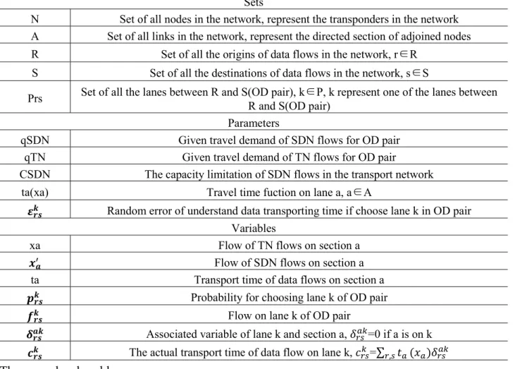
Before formulating the bi-level model, we abstract flow-based SDN into a directed network G={N, A}, and then list some symbols used in the model:

Table 1 Symbols used in bi-level programming model Sets

N Set of all nodes in the network, represent the transponders in the network A Set of all links in the network, represent the directed section of adjoined nodes R Set of all the origins of data flows in the network, r∈R

S Set of all the destinations of data flows in the network, s∈S

Prs Set of all the lanes between R and S(OD pair), k∈P, k represent one of the lanes between R and S(OD pair)

Parameters

qSDN Given travel demand of SDN flows for OD pair qTN Given travel demand of TN flows for OD pair

CSDN The capacity limitation of SDN flows in the transport network ta(xa) Travel time fuction on lane a, a∈A

𝜺_𝒓𝒔𝒌 _{Random error of understand data transporting time if choose lane k in OD pair} Variables

xa Flow of TN flows on section a 𝒙𝒂′ Flow of SDN flows on section a

ta Transport time of data flows on section a 𝒑𝒓𝒔𝒌 Probability for choosing lane k of OD pair 𝒇_𝒓𝒔𝒌 _{Flow on lane k of OD pair}

𝜹_𝒓𝒔𝒂𝒌 _{Associated variable of lane k and section a, 𝛿}

𝑟𝑠𝑎𝑘=0 if a is on k 𝒄_𝒓𝒔𝒌 _{The actual transport time of data flow on lane k, 𝑐}

𝑟𝑠𝑘=∑ 𝑡𝑟,𝑠 𝑎(𝑥𝑎)𝛿𝑟𝑠𝑎𝑘 The upper-level problem:

We aims to minimize the total travel time of entire network, thus the upper-level problem can be formulated as: ' ' min _{a a}( )_{a a a}( )_a a A a A z x t x x t x   







(1) s.t. 𝑓_𝑟𝑠𝑘 _{≥ 0, r∈R, s∈S, k∈P} rs (2)

28 Prs k rs SDN k f q  



, r∈R, s∈S (3) ' , , rs k ak a rs rs r s R S k P x f    

 

, a∈A (4) 𝑥_𝑎′ _{≤CSDN (5)}

The objective function (1) represents the total travel time where xa is determined by the lower-level SUE problem which will be presented later. Constraint (3) (4) ensures to meet the demand of the flows. Constraint (5) guarantees that the total flow does not exceed the capacity limitation.

The lower-level problem:

We use SUE model based on Logit mounted to formulate the lower-level problem, we assume that the random error 𝜀𝑟𝑠𝑘 , r∈R, s∈S, k∈Prs of understand data transporting time is independent identically distributed, mean value equals zero, and is random variable who obey Gumbel probability distribution, then based on random utility probability and utility maximization principle we know that probability of lane choosing can be given by a Logit formula[10]_:

exp( ) exp( ) rs k k rs rs l rs l P c p c      



, r∈R, s∈S, k,l∈Prs

In this formula, non-negative parameter θ represents the understand indeterminacy of data flows’ transporting time. The random error 𝜀𝑟𝑠𝑘 , r∈R, s∈S, k∈Prs is a Gumbel probability variable, therefore bigger value of θ means flows knows better about the condition of the network, thus flows have more accurate estimate on the data transporting time. For example, when θ→∞, flows know exactly what condition it is in the network, they all choose the shortest path, which in the end reaches UE balance.

The problem can be formulated as follows:

0 , , 1 min a ( ) ln rs x _{k k} a rs rs a A r s R S k P Z t w dw f f



   







 

₍₆₎ s.t. rs k rs TN k P f q  



, r∈R, s∈S, k∈Prs 𝑓_𝑟𝑠𝑘_{≥0, r∈R, s∈S, k∈Prs} , , rs k ak a rs rs r s R S k P x f    

 

, a∈A

29

3.3 Solution Method for Model

Sheffi(1985)[9] _{has proved that the Hessian matrix of function (6) is usually not positive definite, but}

it will be positive definite on SUE solution point, which means this function is strictly convex on solution point. Thus, the SUE solution point is a local minimum of the optimization problem.

The mechanism of the model shows as follows: the lower-level obtain variable xa, which is the

resources occupation situation of CN flows under UE balance, according to its objective function. The variable then is used as the initial value of capacity constrain in upper-level optimization problem. The upper-level obtain variable 𝑥_𝑎′_{, which is the resources occupation situation of SDN flows of} system optimization balance. The variable directly influences the lower-level.

In this paper, we use tabu search algorithm[11] _{to solve the bi-level programming model, and use Bell’s}

Logit mounted algorithm[12] _{to solve the lower-level model.}

Bell’s algorithm does not need to enumerate the lanes, and it takes all the possibility into consideration. The set of lane only related to the structure of the network, and has nothing to do with the flow distribution.

Tabu search algorithm is similar to simulated annealing algorithm and genetic algorithm, its relevant parameter influences the operation effect.

At first, we convert the upper-level model into an extremum without constraint; we use penalty function[13] _{to realize this:}

2 2 1 max ( ) ( ) {max [0, ( )] } 2 a a a a a a Y Z x x C p   



    (7)

The basic idea of the algorithm is to select the initial value of capacity constrain, work out the neighborhood of the solution: N(t). Solve the lower-level model to obtain the flow of section, substitute the value of the flow into function (7), we then work out the feasible solution. After that, we search the best solution from a new start point until we obtain the solution of bi-level programming model.

The concrete steps are as follows:

step 0. Set capacity constrain’s initial value is, at this time elements of value zero. Set 𝜏_𝑎(0)=(0,0,0,0,0), solve the problem of lower-level to obtain the value of 𝑥_𝑎(0) and 𝑞_𝑎(0), substitute the values into objective function of upper-lower-level level to obtain Z(𝑡_𝑎(0)). Set the tabu list empty, i=1.

step 1. Expand the neighborhood of 𝜌_𝑎(𝑖), the expand rules are to change only one section’s value each time. If the value of section in 𝜌_𝑎(𝑖) changes from 1 to 0, then this section does not need SDN flows to allocate the flow. Otherwise if 𝜌_𝑎(𝑖) changes from 0 to 1, then randomly generate value based on 𝜏_𝑎(𝑖),

𝜏_𝑎(𝑖+1) = 𝜏_𝑎(𝑖)+ 𝛿[−𝑗, 𝑗], parameter δ is the step size in search. Respectively determine 𝑥_𝑎(𝑖+1) and

𝑞_𝑎(𝑖+1), substitute them into objective function of upper-level to obtain Z(𝑡_𝑎(𝑖+1)), set the value which make the objective maximum as candidate solution.

step 2. Judge the section flow under current state to see if it meets the requirement of capacity constraint. If does, then the candidate solution is the solution we need, update tabu list and the optimal state. If not, then set the optimum solution of taboo object as the solution, update tabu list.

step 3. Set maximum searching times 𝑛_𝑚𝑎𝑥 , if we can’t improve the optimum solution within 𝑛_𝑚𝑎𝑥

times, and then stop the algorithm.

4.

Computational Examples

In order to verify the algorithm validity, we adopt experiment network which is designed by Suwansirikul(1987)[14]_{, showed in Fig. 2. There are 4 nodes, 5 sections and 3 lanes in the network.}

30

We suppose that the quantity demanded is 100, forwarding time function of section a is 𝑡𝑎(𝑥𝑎), and we use function BPR who adds parameter 𝑦𝑎:

0 4

( , ) [1 0.15( / ( )) ]

a a a a a a a

t x y t  x c  y

𝑡𝑎0 is free travel time of section a, 𝑥𝑎 is flow of section a, 𝑐𝑎 is maximum traffic capacity of section a, 𝑦𝑎 is added traffic capacity value of section a.

Fig. 2. Experiment network Objective function is:

2

( ( ), ) ( ) 1.5 ( )

a a a a a a

a a

D



t x y y x y 



h y

The values and parameter ℎ_𝑎 are shown in Tab. 2.

Table 2 Free travel time, maximum capacities and parameter

parameters sections

1 2 3 4 5

𝑡_𝑎(0)/min 4 6 2 5 3

𝑐𝑎/(pcu h-1) 40 40 60 40 40

ℎ_𝑎 2 2 1 2 2

Here are two tables(Tab. 3and Tab.4) which show the results before and after the flow allocation optimization.

Table 3 Results before flow allocation optimization

Before x1 x2 x3 x4 x5

UE 52.53 47.47 5.72 46.81 53.19

Logit-SUE 55.58 44.12 13.18 42.70 57.30

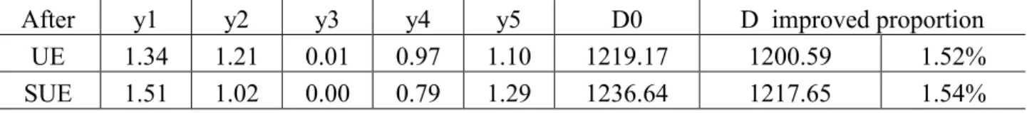
In order to clearly show the results, we show the improved proportion of the optimization. Its computing method is:

Improved proportion=𝐷0−𝐷

𝐷0 ×100%

𝐷₀ is the value of objective function before the optimization, D is the value after optimization. Table 4 Results after flow allocation optimization

After y1 y2 y3 y4 y5 D0 D improved proportion

UE 1.34 1.21 0.01 0.97 1.10 1219.17 1200.59 1.52%

31

From the data above we know that the bi-level programming model optimized the flow allocation of the network.

5.

Conclusion

In this paper, we have built a bi-level programming model in flow-based hybrid SDN, found out the appropriate arithmetic to solve the model. The model has accurately described the interaction of SDN and TN flows in flow-based hybrid SDN. The arithmetic used in this paper has an advantage over other ones. We achieve our aim to optimize the whole network.

Acknowledgments

This work was supported by the Natural Science Foundation of China(NO. 61402266), Natural Science Foundation of Shandong Province, China(NO. ZR2012MF013) and Social Science Fund Project of China(NO. 14BTQ049).

Author Mingchun Zheng is Corresponding Author.

References

[1]S. Sezer et al. Are We Ready for SDN? Implementation Challenges for Software-defined Networks. IEEE Communications Magazine, July 2013.

[2]Stefano V et al. Opportunities and Research Challenges of Hybrid Software Defined Networks. CCR, 2014..

[3]Open Networking Foundation. Outcomes of the Hybrid Working Group. 2013.

[4]C. Y. Heng, S. Kadula, R. Mahajuan et al. Achieving High Utilization with Software-driven Wan. in SIGCOMM, 2013.

[5]S. Agarwl, M. Kodialam, and T. Lakshman. Traffic engineering in software defined networks. INFOCOM, 2013.

[6]McKeown N, Anderson T, Balakrishnan H et al. OpenFlow: Enabling innovation in campus networks. ACM SIGCOMM Computer Communication Review, 2008, 38(2): 69-74.

[7]Balazs Sonkoly, Andras Fulyas. Integrated OpenFlow Virtualization Framework with Fexible Data. Controland Management Function. IEEE INFOCOM(Demo) Orlando, Florida, USA, Mar. 2012.

[8]Wardrop J. Some Theoretical Aspects of Road Traffic Research[C]//Proceedings of the Institution of Civil Engineers, Part Ⅱ, 1952: 325-378.

[9]Sheffi Y. Urban Transportation Networks: Equilibrium Analysis with Mathematical Programming Methods[M]. Prentice Hall, 1985.

[10]Chief-Hua Wen, Frank S Koppelman. The Generalized Nested Logit Model[J]. Transportation Research Part B, 2001, 35(7): 627-641.

[11]Thamilselvan R, Balasubramanie P. A Genetic Algorithm with a Tabu Search for Traveling Salesman Problem[J]. International Journal of Recent Trends in Engineering, 2009, 1(1): 607-610.

[12]Bell M G H. Alternatives to Dial’s Logit Assignment Algorithm. Transportation Research, 1995b, 29B, 287-295.

[13]Bazaraa M, Sherali H D, Shetty C M. Nonlinear Programming: Theory and Algorithms (2nd ed). 1993, New York: Wiley.

[14]Suwansirikul C, Friesz T L, Tobin R L. Equilibrium Decomposed Optimization: A Heuristic for the Continuous Equilibrium Network Design Problem[J]. Transportation science, 1987, 21(4): 254-263.