POLITECNICO DI TORINO
Repository ISTITUZIONALE
Frequent Itemsets Mining for Big Data: A Comparative Analysis / APILETTI, DANIELE; BARALIS, ELENA MARIA; CERQUITELLI, TANIA; GARZA, PAOLO; PULVIRENTI, FABIO; VENTURINI, LUCA. In: BIG DATA RESEARCH. -ISSN 2214-5796. - STAMPA. - 9:C(2017), pp. 67-83.
Original
Frequent Itemsets Mining for Big Data: A Comparative Analysis
elsevier Publisher: Published DOI:10.1016/j.bdr.2017.06.006 Terms of use: openAccess Publisher copyright
-(Article begins on next page)
This article is made available under terms and conditions as specified in the corresponding bibliographic description in the repository
Availability:
This version is available at: 11583/2680344 since: 2017-09-27T11:33:43Z Elsevier Inc.
Frequent Itemsets Mining for Big Data: a comparative
analysis
Daniele Apiletti, Elena Baralis, Tania Cerquitelli, Paolo Garza, Fabio Pulvirenti∗
, Luca Venturini
Politecnico di Torino, Dipartimento Automatica e Informatica, Torino, Italy
Abstract
Itemset mining is a well-known exploratory data mining technique used to discover interesting correlations hidden in a data collection. Since it supports different targeted analyses, it is profitably exploited in a wide range of differ-ent domains, ranging from network traffic data to medical records. With the increasing amount of generated data, different scalable algorithms have been developed, exploiting the advantages of distributed computing frameworks, such as Apache Hadoop and Spark.
This paper reviews Hadoop- and Spark-based scalable algorithms address-ing the frequent itemset minaddress-ing problem in the Big Data frameworks through both theoretical and experimental comparative analyses. Since the itemset mining task is computationally expensive, its distribution and parallelization strategies heavily affect memory usage, load balancing, and communication costs. A detailed discussion of the algorithmic choices of the distributed
∗Corresponding author
Email addresses: [email protected](Daniele Apiletti),
[email protected](Elena Baralis),[email protected](Tania Cerquitelli), [email protected](Paolo Garza),[email protected] (Fabio Pulvirenti),[email protected](Luca Venturini)
methods for frequent itemset mining is followed by an experimental anal-ysis comparing the performance of state-of-the-art distributed implementa-tions on both synthetic and real datasets. The strengths and weaknesses of the algorithms are thoroughly discussed with respect to the dataset features (e.g., data distribution, average transaction length, number of records), and specific parameter settings. Finally, based on theoretical and experimental analyses, open research directions for the parallelization of the itemset mining problem are presented.
Keywords: Big Data, Frequent itemset mining, Hadoop and Spark platforms
1. Introduction
In recent years, the increasing availability of huge amounts of data has changed the importance of data analytic systems for Big Data and the in-terest towards data mining, an important set of techniques useful to extract effective and usable knowledge from data. On the one hand, the Big Data analytics scenario is very challenging for researchers. Indeed, the application of traditional data mining techniques to big volumes of data is not straight-forward and some of the most popular techniques had to be redesigned from scratch to fit the new environment. On the other hand, companies are inter-ested in the strategic benefits that Big Data could deliver. Data mining, to-gether with machine learning [1], is the main research area on which Big Data analytics rely. It includes (i) clustering algorithms to discover hidden struc-tures in unlabeled data [2], (ii) frequent itemsets mining and association rule mining techniques to discover interesting correlations and dependencies [3],
and (iii) supervised algorithms to infer models from labeled datasets and use them to predict the label of new data [4].
Several traditional centralized mining algorithms have been proposed. They are very efficient when the datasets can be completely loaded in main memory. However, they cannot cope with Big Data, because they are not designed for a parallel and distributed environment. The recent shift towards horizontal scalability has highlighted the need of distributed/parallelized data mining algorithms able to exploit the available hardware resources and distributed Big Data frameworks (e.g., Apache Hadoop [5], Apache Spark [6]). In this survey, we focus on distributed/parallel itemset min-ing algorithms in the Big Data context because they represent exploratory approaches widely used to discover frequent co-occurrences from the data. These algorithms have been widely exploited in different application do-mains (e.g., network traffic data [7], healthcare [8], biological data [9], energy data [10], images [11], open linked data [12], document and data summariza-tion [13, 14, 15]).
The parallelization of the frequent itemset mining problem in a dis-tributed environment by means of the MapReduce programming paradigm and a Big Data framework is not an easy task. The main challenge is devis-ing a smart partitiondevis-ing of the problem in independent subproblems, each one based on a subset of the data, to exploit the computation power of a cluster of servers in parallel. In the following, we will describe how this prob-lem has been addressed so far and which are pros and cons of the current MapReduce- and RDD-based parallel algorithms by taking into considera-tion load balancing and communicaconsidera-tion costs, which are two very important
issues in the distributed domain. They are strictly related to the adopted parallelization strategy and usually represent the main bottlenecks of parallel algorithms.
The contributions of this survey are the followings.
• A theoretical analysis of the algorithmic choices that have been pro-posed to address the itemset mining problem in the Big Data context by means of MapReduce, with the analysis of their expected impact on main memory usage, load balancing, and communication costs.
• An extensive evaluation campaign to assess the reliability of our expec-tations. Precisely, we ran more than 300 experiments on 14 synthetic datasets and 2 real datasets to evaluate the execution time, load bal-ancing, and communication costs of five state-of-the-art parallel itemset mining implementations.
• The identification of strengths and weaknesses of the algorithms with respect to the input dataset features (e.g., data distribution, average transaction length, number of records), and specific parameter settings.
• The discussion of promising open research directions for the paralleliza-tion of the itemset mining problem.
This paper is organized as follow. Section 2 briefly introduces the Hadoop and Spark frameworks, while Section 3 introduces the background about the itemset mining problem, providing the main definitions and a brief descrip-tion of the state-of-the-art centralized itemset mining algorithms. Secdescrip-tion 4 describes the algorithmic strategies adopted so far to partition and parallelize
the frequent itemset mining problem by means of the MapReduce paradigm, while Section 5 describes the state-of-the-art distributed algorithms and their implementations. In Section 6 we benchmark the selected algorithms with a large set of experiments on both real and synthetic datasets. Section 7 summarizes the concrete and practical lessons learned from our evaluation analysis, while Section 8 discusses the open issues raised by the experimen-tal validation of the theoretical analysis, highlighting some possible research directions to support a more effective and efficient data mining process on Big Data collections.
2. Apache Hadoop and Spark
The availability of increasing amounts of data has highlighted the need of distributed algorithms able to scale horizontally. To support the design and implementation of these algorithms, the MapReduce [16] programming paradigm and the Apache Hadoop [5] distributed platform have been com-monly used in the last decade. In the last couple of years, instead, Apache Spark [6] has become the favorite distributed platform for large data analyt-ics, outperforming Hadoop thanks to its distributed dataset abstraction.
The success of Hadoop and Spark is mainly due to their data locality paradigm. The basic idea consists in processing data in the same node storing it instead of sending large amounts of data on the network.
Hadoop and Spark support the MapReduce paradigm, a distributed pro-gramming model introduced by Google [16]. A MapReduce application con-sists of two main phases, named map and reduce. The map phase applies a map function on the input data and, after processing them, it emits a set of
key-value pairs. To parallelize the execution of the map phase, each node of the cluster applies the map function in isolation on a disjoint subset of the input data. Then, the map results are exchanged among the cluster nodes and the reduce phase is run. Specifically, the reduce phase considers one unique key at a time and iterates through the values that are associated with that key to emit the final results. Also the reduce phase can be parallelized by assigning to each node a subset of keys.
MapReduce-based programs implemented on Hadoop do not fit well it-erative processes because each iteration requires a new reading phase from disk. This feature is critical when dealing with huge datasets. This issue motivated the improvements introduced by Spark, which enables the nodes of the cluster to cache data and intermediate results in memory, instead of reloading them from the disk at each iteration. This goal is achieved through the introduction of the Resilient Distributed Dataset (RDD) data structure, which is a read-only partitioned collection of records distributed across the nodes of the cluster. An RDD, when it is reused multiple times, is cached in the main memory of the nodes to avoid the overhead given by multiple reads from disk.
2.1. Hadoop and Spark Data Mining and Machine Learning Libraries In recent years the success of Hadoop and Spark was supported by the introduction of open source data mining and machine learning libraries. Ma-hout [17] for Hadoop has been one of the most popular collection of Machine Learning algorithms, providing distributed implementations of well-known clustering, classification, and itemset mining algorithms. All the current im-plementations are based on MapReduce. MADlib [18], instead, provides a
SQL toolkit of algorithms that run over Hadoop. Finally, MLLib [19] is the Machine Learning and data mining library developed on Spark. MLlib allows researchers to exploit Spark special features to implement all those applications that can benefit from them, e.g. faster iterative procedures. 2.2. Distributed data mining approaches based on MPI and GPUs
Hadoop and Spark are not the only frameworks supporting the paralleliza-tion of data mining algorithms and their distributed execuparalleliza-tion. Specifically, the distributed execution of the data mining algorithms has been addressed also by using solutions based on Message Passing Interface (MPI) [20], one of the most adopted framework in academic environment, or more recent hardware components, such as GPUs.
For instance, the solutions proposed in [21, 22, 23, 24, 25, 26] are MPI-based solutions for the itemset mining problem, whereas solutions like [27, 28, 29] take advantage of GPU-based commodity cluster. A comparative analysis of the GPU-based solutions is reported in [30].
The focus of this work is the comparison of the MapReduce-based ap-proaches. Hadoop and Spark have been widely adopted in the research en-vironment [31, 32, 33]. The reasons are partly related to the easier data management and better fault tolerance [34, 34, 26] but, above all, these frameworks allow the development of parallel algorithms by unexperienced users [31].
3. Frequent itemset mining
A frequent itemset represents frequently co-occurring items in a transac-tional dataset. More formally, letI be a set of items. A transactional dataset
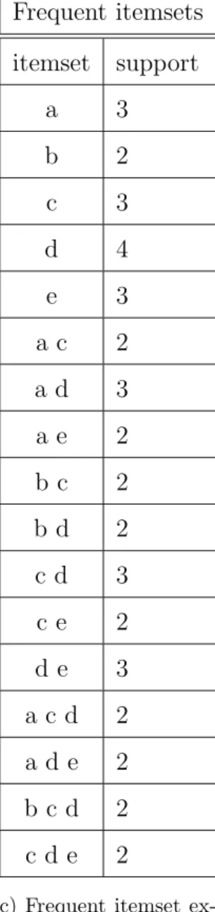
D tid items 1 a b c d 2 a c d e 3 b c d e 4 a d e (a) Horizontal representation of D T T item tidlist a 1,2,4 b 1,3 c 1,2,3 d 1,2,3,4 e 2,3,4 (b) Transposed representation ofD Frequent itemsets itemset support a 3 b 2 c 3 d 4 e 3 a c 2 a d 3 a e 2 b c 2 b d 2 c d 3 c e 2 d e 3 a c d 2 a d e 2 b c d 2 c d e 2
(c) Frequent itemset ex-tracted from D with a minsup=2
D consists of a set of transactions {t1, . . . , tn}. Each transaction ti ∈ D is
a collection of items (i.e., ti ⊆ I) and is identified by a transaction
identi-fier (tidi). Figure 1a reports an example of a transactional dataset with 4
transactions.
An itemset I is defined as a set of items (i.e., I ⊆ I) and is character-ized by a support value, which is denoted by sup(I) and defined as the ratio between the number of transactions in D containing I and the total num-ber of transactions in D. In the example dataset in Figure 1a, for example, the support of the itemset {a,c,d} is 50% (2/4). This value represents the frequency of occurrence of the itemset in the dataset. An itemset I is consid-ered frequent if its support is greater than a user-provided minimum support threshold minsup. Figure 1c reports the frequent itemset extracted from D
with a minsup value equal to 50% (i.e., an absolute support equal to 2). Given a transactional datasetDand a minimum support thresholdminsup, the Frequent Itemset Mining [3] problem consists in extracting the complete set of frequent itemsets from D.
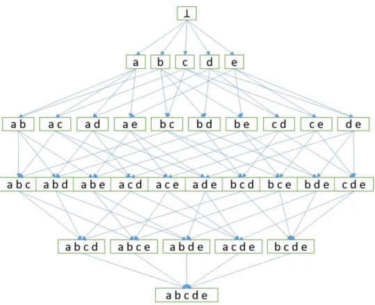
The dimension of the search space can be represented as a lattice, whose top is an empty set. Its size increases exponentially with the number of items [35, 36]. In Figure 2, the lattice related to our running example is shown.
In this paper, we focus on closed itemsets. Closed itemsets [37] are a particular and valuable subset of frequent itemsets, being a concise but com-plete representation of the set of frequent itemsets. Precisely, an itemset I is closed if none of its supersets (i.e. the set of itemsets which include I) has the same support count as I. For instance, in our running example, given
Figure 2: Lattice representing the search space based on the items appearing in the ex-ample dataset D
a minsup = 2, the itemset {a,d} is a closed frequent itemset (support=3). The itemset {a,c}, instead, is a frequent itemset (support=2), but it is not closed because of the presence of the itemset {a,c,d} (support=2).
A transactional dataset can also be represented in a vertical format, in which each row represents an itemiand the list of tids of the transactions in which it appears, also calledtidlist({i}). For instance, the tidlist of the item a in the example dataset D is {1,2,4}. Figure 1b reports the transposed representation of the running example reported in Figure 1a. The main
advantage of the vertical format is the possibility to obtain the tidlist of an itemset by intersecting the tidlists of the included items, without the need of a full scan of the dataset.
3.1. Centralized algorithms
The search space exploration strategies of the distributed approaches are often inspired by the solutions adopted by the centralized approaches. Hence, this section shortly introduces the main strategies of the centralized itemset mining algorithms. This introduction is useful to better understand the algorithmic choices behind the distributed algorithms.
The frequent itemset mining task is challenging in terms of execution time and memory consumption because the size of the search space is expo-nential with the number of items of the input dataset [35]. Two main search space exploration strategies have been proposed: (i) level-wise or breadth-first exploration of the candidate itemsets in the lattice and (ii) depth-breadth-first exploration of the lattice.
The most popular representative of the breadth-first strategy is Apri-ori [38]. Starting from single items, it iteratively generates and counts the support of the candidate itemsets of size k+ 1 from the frequent itemsets of size k. At each iteration k, the supports of the candidate itemsets of length k are counted by performing a new scan of the input dataset. The search space is pruned by exploiting the downward-closure property, which guarantees that all the supersets of an infrequent itemset are infrequent too. Specifically, the downward-closure property allows pruning the set of candi-date itemsets of lengthk+ 1 by considering the frequent itemsets of lengthk. The Apriori algorithm is significantly affected by the density of the dataset.
The higher the density of the dataset, the higher the number of frequent itemsets and hence the amount of candidate itemset stored in main mem-ory. The problem becomes unfeasible when the number of candidate itemsets exceeds the size of the main memory.
More efficient and scalable solutions exploit the depth-first visit of the search space. FP-Growth [39], which uses a prefix-tree-based main memory compressed representation of the input dataset, is the most popular depth-first based approach. The algorithm is based on a recursive visit of the tree-based representation of the dataset with a “divide and conquer” ap-proach. In the first phase the support of each single item is counted and only the frequent items are stored in the “frequent items table” (F-list). This information allows pruning the search space by avoiding the analysis of the itemsets extending infrequent items. Then, the FP-tree, that is a compact representation of the dataset, is built exploiting the F-list and the input dataset (together they compose the “header table”) . Specifically, each transaction is included in the FP-tree by adding or extending a path on the tree, exploiting common prefixes. Once the FP-tree associated with the input dataset is built, FP-growth recursively splits the itemset mining problem by generating conditional FP-trees and visiting them. Given an arbitrary prefix p, where p is a set of items, the conditional FP-tree with respect to p, also called projected dataset with respect top, is substantially the compact repre-sentation of the transactions containingp. Each conditional FP-tree contains all the knowledge needed to extract all the frequent itemsets extending its prefix p. FP-growth decomposes the initial problem by generating one con-ditional FP-tree for each itemt i and invoking the itemset mining procedure
on each of them, in a recursive depth-first fashion.
FP-growth suits well dense datasets, because they can be effectively and compactly represented by means of the FP-tree data structure. Differently, with sparse datasets, the compressions benefits of the FP-tree are reduced because there will be a higher number of branches [3] (i.e., a large number of subproblems to generate and results to merge).
Another very popular depth-first approach is the Eclat algorithm [40]. It performs the mining from a vertical transposition of the dataset. In the verti-cal format, each transaction includes an item and the transaction identifiers (tid) in which it appears (tidlist). After the initial dataset transposition, the search space is explored in a depth-first manner similar to FP-growth. The algorithm is based on equivalence classes (groups of candidate itemsets sharing a common prefix), which allows smartly merging tidlists to select fre-quent itemsets. Prefix-based equivalence classes are mined independently, in a “divide and conquer” strategy, still taking advantage of the downward clo-sure property. Eclat is relatively robust to dense datasets. It is less effective with sparse distributions, because the depth-first search strategy may require generating and testing more (infrequent) candidate itemsets with respect to Apriori-like algorithms [41].
4. Itemset mining parallelization strategies
Two main algorithmic approaches are proposed to address the parallel execution of the itemset mining algorithms by means of the MapReduce paradigm. They are significantly different because (i) they use different so-lutions to split the original problem in subproblems and (ii) make different
assumptions about the data that can be stored in the main memory of each independent task.
Data split approach. It splits the problem in “similar” subproblems, ex-ecuting the same function on different data chunks. Specifically, each subproblem computes the local supports of all candidate itemsets on one chunk on the input dataset (i.e., each subproblem works on the complete search space but on a subset of the input data). Finally, the local results (i.e., the local supports of the candidate itemsets) emit-ted by each subproblem/task are merged to compute the global final result (global support of each itemset). The main assumptions of this approach are that (i) the problem can be split in “similar’ subproblems working on different chunks of the input data and (ii) the set of candi-date itemsets is small enough that it can be stored in the main memory of each task.
Search space split approach. It splits the problem by assigning to each subproblem the visit of a subset of the search space (i.e., each subprob-lem visits a part of the lattice). Specifically, this approach generates, from the input distributed dataset, a set of projected datasets, each one small enough to be stored in the main memory of a single task. Each projected dataset contains all the information that is needed to extract a subset of itemsets (i.e., each dataset contains all the infor-mation that is needed to explore a part of the lattice) without needing the contribution of the results of the other tasks. The final result is the union of the itemset subsets mined from each projected dataset.
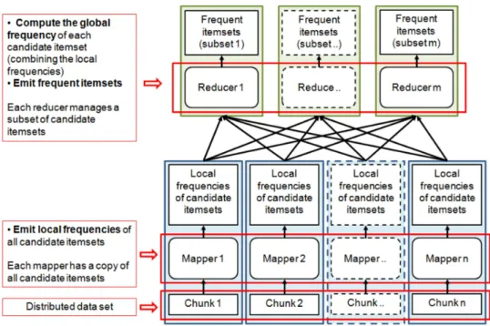
Figure 3: Itemset mining parallelization: Data split approach
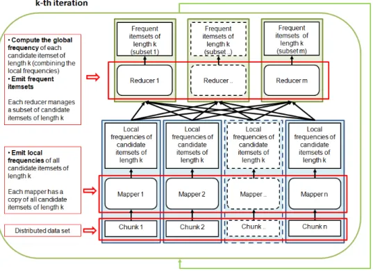
Figures 3 and 5 depict the first and the second parallelization strategies, respectively. In the data split approach (Figure 3), the map phase computes the local supports of the candidate itemsets in its data chunk (i.e., each mapper runs a “local itemset mining extraction” on its data chunk). Then, the reduce phase merges the local supports of each candidate itemset to compute its global support. This solution requires each mapper to store a copy of the complete set of candidate itemsets (i.e., a copy of the lattice). This set must fit in the main memory of each mapper. Since the complete set of candidate itemsets is usually too large to be stored in the main memory of a single mapper, an iterative solution, inspired by the level-wise centralized itemset mining algorithms, is used. Figure 4 reports the iterative solution. At each iteration k only the subset of candidates of lengthk are considered and
Figure 4: Itemset mining parallelization: Iterative Data split approach
hence stored in the main memory of each mapper. This approach, thanks also to the exploitation of the apriori-principle to reduce the size of the candidate sets, allows obtaining subsets of candidate itemsets that can be loaded in the main memory of every mapper.
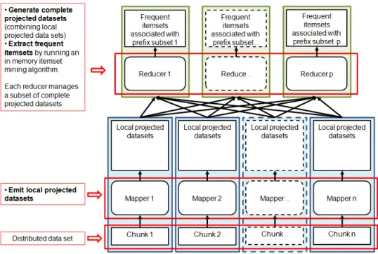
In the search space split approach (Figure 5), the map phase generates a set of local projected datasets. Specifically each mapper generates a set of local projected datasets based on its data chunk. Each local projected dataset is the projection of the input chunk with respect to a prefix p.1
1
Note that the projected datasets can overlap because the transactions associated with two distinct prefixesp1andp2can be overlapped.
Figure 5: Itemset mining parallelization: Search space split approach
Then, the reduce phase merges the local projected datasets to generate the complete projected datasets. Each complete projected dataset is provided as input to a standard centralized itemset mining algorithm running in the main memory of the reducer and the set of frequent itemsets associated to it are mined. Each reducer is in charge of analyzing a subset of complete projected datasets by running the itemset mining phase on one complete projected dataset at a time. Hence, the main assumption, in this approach, is that each complete projected dataset must fit in the main memory of a single reducer.
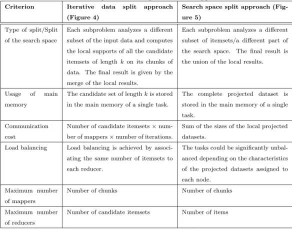
Table 1 summarizes the main characteristics of the two parallelization approaches with respect to the following criteria: type of split of the problem, usage of main memory, communication costs, load balancing, and maximum
Table 1: Comparison of the parallelization approaches.
Criterion Iterative data split approach (Figure 4)
Search space split approach (Fig-ure 5)
Type of split/Split of the search space
Each subproblem analyzes a different subset of the input data and computes the local supports of all the candidate itemsets of lengthk on its chunks of data. The final result is given by the merge of the local results.
Each subproblem analyzes a different subset of itemsets/a different part of the search space. The final result is the union of the local results.
Usage of main memory
The candidate set of lengthkis stored in the main memory of a single task.
The complete projected dataset is stored in the main memory of a single task.
Communication cost
Number of candidate itemsets×
num-ber of mappers×number of iterations.
Sum of the sizes of the local projected datasets.
Load balancing Load balancing is achieved by associ-ating the same number of itemsets to each reducer.
The tasks could be significantly unbal-anced depending on the characteristics of the projected datasets assigned to each node.
Maximum number of mappers
Number of chunks Number of chunks
Maximum number of reducers
Number of candidate itemsets Number of items
parallelization (i.e. maximum number of mappers and reducers).
Type of split/Split of the search space. The main difference between the two parallelization approaches is the strategy adopted to split the problem in subproblems. This choice has a significant impact on the other criteria. Usage of main memory. The different usage of the main memory of the tasks impact on the reliability of the two approaches. The data split approach assumes that the candidate itemsets of length k can be stored in the main memory of each mapper. Hence, it is not able to scale on dense datasets characterized by large candidate sets. Differently, the search space
split approach assumes that each complete projected dataset can be stored in the main memory of a single task. Hence, this approach runs out of memory when large complete projected datasets are generated.
Communication costs. In a parallel MapReduce algorithm, communica-tion costs are important, because the network can easily become the bottle-neck if large amounts of data are sent on it. The communication costs are mainly related to the outputs of the mappers which are sent to the reducers on the network. For the data split approach the data that is sent on the net-work is linear with respect to the number of candidate itemsets, the number of mappers, and the number of iterations. Differently, for the search space approach, the amount of data emitted by the mappers is equal to the size of the projected datasets.
Load balancing. The different split of the problem in subproblems signifi-cantly impacts on load balancing. For the data split approach, the execution time of each mapper is linear with respect to the number of input transactions and the execution time of each reducer is linear with respect to the number of assigned itemsets. Hence, the data split approach can easily achieve a good load balancing by assigning the same number of data chunks to each mapper and the same number of candidate itemsets to each reducer. Differently, the search space split approach is potentially unbalanced. In fact, each subprob-lem is associated with a different subset of the lattice, related to a specific projected dataset and prefix, and, depending on the data distribution, the complexity of the subproblems can significantly vary. A smart assignment of a set of subproblems to each node would mitigate the unbalance. How-ever, the complexity of the subproblems is hardly inferable during the initial
assignment phase.
Maximum number of mappers and reducers. The two approaches are significantly different in terms of “maximum parallelization degree”, at least in terms of number of maximum exploitable reducers. The maximum parallelization of the map phase is equal to the number of data chunks for both approaches. Differently, the maximum parallelization of the reduce phase is equal to the number of candidate itemsets for the data split approach, because potentially each reducer could compute the global frequency of a single itemset, whereas it is equal to the number of global projected datasets for the second approach, which can be at most equal to the number of items. Since the number of candidate itemsets is greater than the number of items, the data split approach can potentially reach a higher degree of parallelization with respect to the search space split approach.
The two parallelization approaches are used to design efficient parallel im-plementations of well-known centralized itemset mining algorithms. Specif-ically, the data split approach is used to implement the parallel versions of level-wise algorithms (like Apriori [38]), whereas the search space split approach is used to implement parallel versions of depth-first recursive ap-proaches (like FP-growth [39] and Eclat [40]).
5. Distributed itemset mining algorithms
This section describes the algorithms, and available implementations, rep-resenting the state-of-the-art solutions in the parallel frequent itemset min-ing context. We considered the followmin-ing algorithms: YAFIM [42], PFP [43], BigFIM [44], and DistEclat [44]. The only algorithm which is lacking a
pub-licly available implementation is YAFIM. Among the considered algorithms, YAFIM belongs to the ones based on the data split approach, while PFP and DistEclat are based on the search space split approach. Finally, BigFIM mixes the two strategies, aiming at exploiting the pros of them. For PFP we selected two popular implementations: Mahout PFP and MLlib PFP, which are based on Hadoop and Spark, respectively. The description of the four selected algorithms and their implementations are reported in the following subsections.
5.1. YAFIM
YAFIM[42] is an Apriori distributed implementation developed in Spark. The iterative nature of the algorithm has always represented a challenge for its application in MapReduce-based Big Data frameworks. The reasons are the overhead caused by the launch of new MapReduce jobs and the require-ment to read the input dataset from disk at each iteration. YAFIM exploits Spark RDDs to cope with these issues. Precisely, it assumes that all the dataset can be loaded into an RDD to speed up the counting operations. Hence, after the first phase in which all the transactions are loaded in an RDD, the algorithm starts the iterative Apriori algorithm organizing the can-didates in a hash tree to speed up the search. Being strongly Apriori-based, it inherits the breadth-first strategy to explore and partition the search space and the preference towards sparse data distributions. YAFIM exploits the Spark “broadcast variables abstraction” feature, which allows programmers to send subsets of shared data to each slave only once, rather than with every job that uses those subset of data. This implementation mitigates commu-nication costs (reducing the inter job commucommu-nication), while load balancing
is not addressed.
5.2. Parallel FP-growth (PFP)
Parallel FP-growth[43], called PFP, is a distributed implementation of FP-growth that exploits the MapReduce paradigm to extract thek most fre-quent closed itemsets. It is included in the Mahout machine learning Library (version 0.9) and it is developed on Apache Hadoop. PFP is based on the search space split parallelization strategy reported in Section 4. Specifically, the distributed algorithm is based on building independent FP-trees (i.e., projected datasets) that can be processed separately over different nodes.
The algorithm consists of 3 MapReduce jobs.
First job. It builds the F-list, that is used to select frequent items, in a MapReduce “Word Count” manner.
Second job. In the second job, the mappers project with respect to group of items (prefixes) all the transactions of the input dataset to generate the local projected contributions to the projected datasets. Then, the reducers aggregate the projections associated with the items of the same group and build independent complete FP-trees from them. Each complete FP-tree is managed by one reducer, which runs a local main memory FP-growth algorithm on it and extracts the frequent itemsets associated with it.
Third job. Finally, the last MapReduce job selects the top k frequent closed itemsets.
The independent complete FP-trees can have different characteristics and this factor has a significant impact on the execution time of the mining tasks. As discussed in Section 4, this factor significantly impacts on load balancing. Specifically, when the independent complete FP-trees have different sizes and
characteristics, the tasks are unbalanced because they addresses subproblems with different complexities. This problem could be potentially solved by splitting complex trees in sub-trees, each one associated with an independent subproblem of the initial one. However, defining a metric to split a tree in such a way to obtain sub-mining problems that are equivalent in terms of execution time is not easy. In fact, the execution time of the itemset mining process on an FP-Tree is not only related to its size (number of nodes) but also to other characteristics (e.g., number of branches and frequency of each node). Depending on the dataset characteristics, the communication costs can be very high, especially when the projected the datasets overlap significantly because in that case the overlapping part of the data is sent multiple times on the network.
Spark PFP [19] represents a pure transposition of PFP to Spark. It is included in MLlib, the Spark machine learning library. The algorithm implementation in Spark is very close to the Hadoop sibling. The main difference, in terms of addressed problem, is that MLlib PFP mines all the frequent itemsets, whereas Mahout PFP mines only the topkclosed itemsets. Both implementations, being strongly inspired by FP-growth, keep from the underlying centralized algorithm the features related to the search space exploration (depth-first) and the ability to efficiently mine itemsets from dense datasets.
5.3. DistEclat and BigFIM
DistEclat [44] is a Hadoop-based frequent itemset mining algorithms in-spired by the Eclat algorithm, whereas BigFIM [44] is a mixed two-phase algorithm that combines an Apriori-based approach with an Eclat-based one.
DistEclat is a frequent itemset miner developed on Apache Hadoop. It exploits a parallel version of the Eclat algorithm to extract a superset of closed itemsets
The algorithm mainly consists of two steps. The first step extracts k -sized prefixes (i.e., frequent itemsets of length k) with respect to which, in the second step, the algorithm builds independent projected subtrees, each one associated with an independent subproblem. Even in this case, the main idea is to mine these independent trees in different nodes, exploiting the search split parallelization approach discussed in Section 4.
The algorithm is organized in 3 MapReduce jobs.
First job. In the initial job, a MapReduce job transposes the dataset into a vertical representation.
Second job. In this MapReduce job, each mapper extracts a subset of the k -sized prefixes (k-sized itemsets) by running Eclat on the frequent items, and the related tidlists, assigned to it. The k-sized prefixes and the associated tidlists are then split in groups and assigned to the mappers of the last job. Third job. Each mapper of the last mapReduce job runs the in main memory version of Eclat on its set of independent prefixes. The final set of frequent itemsets is obtained by merging the outputs of the last job.
The mining of the frequent itemsets in two different steps (i.e., mining of the itemsets of length k in the second job and mining of the other fre-quent itemsets in the last job) aims at improving the load balancing of the algorithm. Specifically, the split in two steps allows obtaining simpler sub-problems, which are potentially characterized by similar execution times. Hence, the application is overall well-balanced.
DistEclat is designed to be very fast but it assumes that all the tidlists of the frequent items should be stored in main memory. In the worst case, each mapper needs the complete dataset, in vertical format, to build all the 2-prefixes [44]. This impacts negatively on the scalability of DistEclat with respect to the dataset size. The algorithm inherits from the centralized version the depth-first strategy to explore the search space and the preference for dense datasets.
BigFIM is an Hadoop-based solution very similar to DistEclat. Analo-gously to DistEclat, BigFIM is organized in two steps: (i) extraction of the frequent itemsets of length less than or equal to the input parameter k and (ii) execution of Eclat on the sub-problems obtained splitting the search space with respect to thek-itemsets. The difference lies in the first step, where Big-FIM exploits an Apriori-based algorithm to extract frequent k-itemsets, i.e., it adopts the data split parallelization approach (Section 4). Even if BigFIM is slower than DistEclat, BigFIM is designed to run on larger datasets. The reason is related to the first step in which, exploiting an Apriori-based ap-proach, thek-prefixes are extracted in a breadth-first fashion. Consequently, the nodes do not have to keep large tidlists in main memory but only the set of candidate itemsets to be counted. However, this is also the most critical issue in the application of the data split parallelization approach, because, depending on the dataset density, the set of candidate itemsets may not be stored in main memory.
Because of the two different techniques used by BigFIM in its two main steps (data split and then search space split), in the first step BigFIM achieves the best performance with sparse datasets, while in the second phase it better
fits dense data distributions.
DistEclat and BigFIM are the only algorithms specifically designed for addressing load balancing and communication cost by means of the prefix length parameter k. In particular, the choice of the length of the prefixes generated during the first step affects both load balancing and communica-tion cost.
6. Experimental evaluation
In this section, the results of the experimental comparison are presented. The behaviors of the algorithm reference implementations are compared by considering different data distributions and use cases. The experimental evaluation aims at understanding the relations between the algorithm per-formance and its parallelization strategies. Algorithm perper-formance are eval-uated in terms of (i) efficiency (i.e., execution time and scalability) under different conditions (Sections 6.2-6.8), (ii) load balancing (Section 6.9), and (iii) communication costs (Section 6.10).
6.1. Experimental setup
The experimental evaluation includes the following four algorithms, which are described in Section 5:
• the Parallel FP-Growth implementation provided in Mahout 0.9 (named Mahout PFP in the following) [17],
• the Parallel FP-Growth implementation provided in MLlib for Spark 1.3.0 (named MLlib PFP in the following) [19],
• the June 2015 implementation of BigFIM [45],
• the version of DistEclat downloaded from [45] on September 2015. We recall that Mahout PFP extracts the top k frequent closed itemsets, BigFIM and DistEclat extract a superset of the frequent closed itemsets, while MLlib PFP extracts all the frequent itemsets. To perform a fair com-parison, Mahout PFP is forced to output all the closed itemsets. Addition-ally, in our experiments, the numbers of frequent itemsets and closed itemsets are in the same order of magnitude. Therefore, even if the extraction of the complete set of frequent itemsets is usually more resource-intensive than deal-ing with only the set of frequent closed itemsets, the disadvantages related to the more intensive task performed by MLlib are mitigated2
We defined a common set of default parameter values for all experiments. Specific experiments with different settings are explicitly indicated. The de-fault setting of each algorithm was chosen by taking into account the physical characteristics of the Hadoop cluster, to allow each approach to exploit the hardware and software configuration at its best.
• For Mahout PFP, the default value ofkis set to the lowest value forcing Mahout PFP to mine all frequent closed itemsets.
• For MLlib PFP the number of partitions is set to 6,000. This value has shown to be the best tradeoff among performance and the capacity
2
We recall that the complete set of frequent itemsets can be obtained expanding and combining the closed itemsets by means of a post-processing step. Hence, to obtain the same output, the execution times of Mahout PFP, BigFIM and DistEclat may increase with respect to MLlib PFP
to complete the task without memory issues. In particular, with lower values of the the number of partitions MLlib PFP cannot scale to very long transactions or very low minsup. Higher values, instead, do not lead to better scalability, while affecting performance.
• The default value of the prefix length parameter of both BigFIM and DistEclat is set to 2, which achieves a good tradeoff among efficiency and scalability of the two approaches.
• We did not define a default value of minsup, which is a common pa-rameter of all algorithms, because it is highly related to the data distri-bution and the use case, so this parameter value is specifically discussed in each set of experiments.
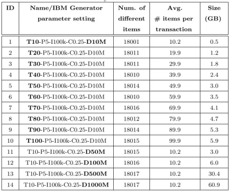
We considered both synthetic and real datasets. The synthetic ones have been generated by means of the IBM dataset generator [46], commonly used for performance benchmarking in the itemset mining context. We tuned the following parameters of the IBM dataset generator to analyze the impact of different data distributions on the performance of the mining algorithms: T = average size of transactions, P = average length of maximal patterns, I = number of different items, C = correlation grade among patterns, and D = number of transactions. The full list of synthetic datasets is reported in Table 2, where the name of each dataset consists of pairs<parameter,value>. Finally, two real datasets have been used to simulate real-life use cases. They are described in Section 6.8.
All the experiments, except the speedup analysis, were performed on a cluster of 5 nodes running the Cloudera Distribution of Apache Hadoop
(CDH5.3.1) [47]. Each cluster node is a 2.67 GHz six-core Intel(R) Xeon(R) X5650 machine with 32 Gigabytes of main memory and SATA 7200-rpm hard disks. The dimension of Yarn containers is set to 6 GB. This value leads to a full exploitation of the resources of our hardware, representing a good trade-off between the amount of memory assigned to each task and the level of parallelism. Lower values would have increased the level of parallelism (i.e. the number of concurrent parallel tasks) at the expense of the tasks avail-able memory and, therefore, their ability to complete the frequent itemset mining. Higher values, instead, would have decreased the maximum level of parallelism.
For the speedup experiments we used a larger cluster of 30 nodes3 with
2.5 TB of total RAM and 324 processing cores provided by Intel CPUs E5-2620 at 2.6GHz, running the same Cloudera Distribution of Apache Hadoop (CDH5.3.1) [47].
From a practical point of view, all the implementations revealed to be quite easy to deploy and use. Actually, the only requirement for all the implementations to be run was the Hadoop/Spark installation (from a single machine scenario to a large cluster). Only the MLlib PFP implementation requires few additional steps and some coding skills, since it is delivered as a library: users must develop their own class and compile it.
6.2. Impact of the minsup support threshold
The minimum support threshold (minsup) has a high impact on the com-plexity of the itemset mining task. Specifically, the lower the minsup, the
3
Table 2: Synthetic datasets
ID Name/IBM Generator Num. of Avg. Size parameter setting different # items per (GB)
items transaction 1 T10-P5-I100k-C0.25-D10M 18001 10.2 0.5 2 T20-P5-I100k-C0.25-D10M 18011 19.9 1.2 3 T30-P5-I100k-C0.25-D10M 18011 29.9 1.8 4 T40-P5-I100k-C0.25-D10M 18010 39.9 2.4 5 T50-P5-I100k-C0.25-D10M 18014 49.9 3.0 6 T60-P5-I100k-C0.25-D10M 18010 59.9 3.5 7 T70-P5-I100k-C0.25-D10M 18016 69.9 4.1 8 T80-P5-I100k-C0.25-D10M 18012 79.9 4.7 9 T90-P5-I100k-C0.25-D10M 18014 89.9 5.3 10 T100-P5-I100k-C0.25-D10M 18015 99.9 5.9 11 T10-P5-I100k-C0.25-D50M 18015 10.2 3.0 12 T10-P5-I100k-C0.25-D100M 18016 10.2 6.0 13 T10-P5-I100k-C0.25-D500M 18017 10.2 30.4 14 T10-P5-I100k-C0.25-D1000M 18017 10.2 60.9
higher the complexity of the mining task [36]. For this reason, this set of experiments uses very low minsup values. Specifically, we have tried to lower as much as possible the minsup values to understand the behavior of the al-gorithms dealing with such challenging tasks. Moreover, the selected minsup values strongly affect the amount of mined knowledge (i.e., the number of mined itemsets).
To avoid the bias due to a specific single data distribution, two different datasets have been considered: Dataset #1 and Dataset #3 (Table 2). They share the same average maximal pattern length (5), the number of different items (100 thousands), the correlation grade among patterns (0.25), and the number of transactions (10 millions). The difference is in the average
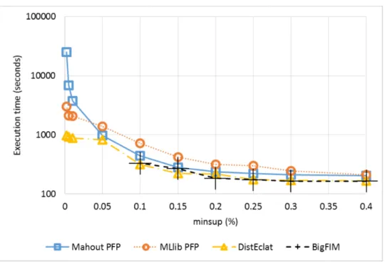
Figure 6: Execution time for different minsupvalues (Dataset #1), average transaction length 10.
transaction length: 10 items for Dataset #1 and 30 items for Dataset #3. Being the other characteristics constant, longer transactions lead to a higher dataset density, which results into a larger number of frequent itemsets.
Figure 6 reports the execution time of the algorithms when varying the minsup threshold from 0.002% to 0.4% and considering Dataset #1. DistE-clat is the fastest algorithm for all the considered minsup values. However, the improvement with respect to the other algorithms depends on the value ofminsup. Whenminsupis greater than or equal to 0.2%, all the implemen-tations show similar performances. The performance gap largely increases with minsup values lower than 0.05%. BigFIM is as fast as DistEclat when minsup is higher than 0.1%, but below this threshold BigFIM runs out of
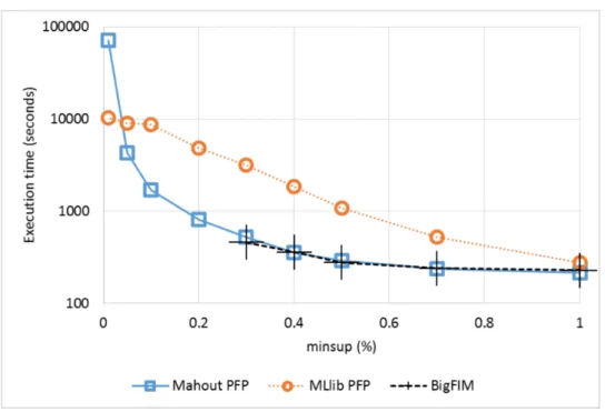
Figure 7: Execution time for different minsupvalues (Dataset #3), average transaction length 30.
memory during the extraction of 2-itemsets.
In the second set of experiments, we analyzed the execution time of the algorithms for different minimum support values on Dataset #3, which is characterized by a higher average transaction length (3 times longer than Dataset #1), and a larger data size on disk, with the same number of trans-actions (10 millions). Since the mining task is more computationally in-tensive, minsup values lower than 0.01% were not considered in this set of experiments, as this has proven to be a limit for most algorithms due to memory exhaustion or too long experimental duration (days). Results are reported in Figure 7. MLlib PFP is much slower than Mahout PFP for most minsupvalues (0.7% and below), and BigFIM, as in the previous experiment,
achieves top-level performance, but cannot scale to low minsup values (the lowest is 0.3%), due to memory constraints during the k-itemset generation phase. Finally, DistEclat was not able to run because the size of the initial tidlists was already too big. Using the data-split approach, instead, BigFIM generates the set of candidates to be tested in independent chunks of the dataset. With a low minsup value, the set of candidates of the first phases is already too large to be stored and tested in each independent task. Overall, as expected, DistEclat is the fastest approach when it does not run out of memory. Mahout PFP is the most reliable implementation across almost all minsup values, even if it is not always the fastest, sometimes with large gaps behind the top performers. MLlib is a reasonable tradeoff choice, as it is constantly able to complete all the tasks in a reasonable time. Finally, BigFIM does not present advantages over the other approaches, being unable to reach low minsupvalues and to provide fast executions.
6.3. Impact of the average transaction length
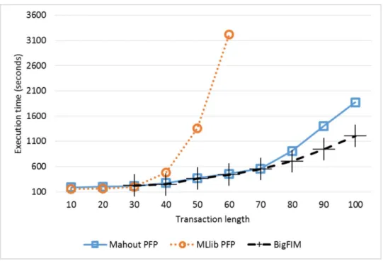
We analyzed the effect of different average transaction lengths, from 10 to 100 items per transaction. We fixed the number of transactions to 10 millions. To this aim, Datasets #1–10 were used (see Table 2). Longer transactions often lead to more dense datasets and a larger number of long frequent itemsets. This generally corresponds to more computationally in-tensive tasks. The execution times obtained are reported in Figure 8 and Figure 9, with a respective minsup value of 1% and 0.1%. In the experiment of Figure 8, BigFIM and DistEclat execution times for transaction length of 10 and 20 are not reported because, for these configurations, no 3-itemsets
Figure 8: Execution time with different average transaction lengths (Datasets #1–10, minsup1%).
are extracted and hence the two algorithms could not complete the mining.4
For higher transaction lengths, DistEclat is not included since it runs out of memory for values beyond 20 items per transaction. The other algorithms have similar execution times for short transactions, up to 30 items. For longer transactions, a clear trend is shown: (i) MLlib PFP is much slower than the others and it is not able to scale for longer transactions, as its execution times abruptly increase until it runs out of memory; (ii) Mahout PFP and BigFIM have a similar trend until 70 items per transactions, when Mahout
4
Due to the absence of a specific test, BigFIM and DistEclat present some issues if no itemsets longer than the value of the prefix length parameter are mined.
Figure 9: Execution time with different average transaction lengths (Datasets #1–10, minsup0.1%).
PFP becomes slower than BigFIM.
The experiments of Figure 9, shows a very similar trend, with exception that also BigFIM is not able to run.
Overall, despite the Apriori-based initial phase, BigFIM proved to be the best scaling approach for very long transactions and a relatively high min-sup. When the minsup is decreased, BigFIM is penalized by the data-split approach which assumes to store all the candidates in each task memory, and only Mahout PFP is able to cope with the complexity of the task.
Figure 10: Execution time with different numbers of transactions (Datasets #1, #11–14, minsup0.4%).
6.4. Impact of the number of transactions
We evaluated the effect of varying the number of transactions, i.e., the dataset size, without changing intrinsic data characteristics (e.g., transac-tion length or data distributransac-tion). The experiments have been performed on Datasets #1, #11–14 have been used (see Table 2), which have a number of transactions ranging from 10 millions to 1 billion. The minsup is set to 0.4%, which is the highest value for which the mining leverages both phases of BigFIM, and it corresponds to the highest value used in the experiments of Section 6.2. Since in the experiment the relative minsup threshold is fixed, from the mining point of view, the search space exploration is similar and not particularly challenging, as shown in Section 6.2. What really affects this
experiment is the algorithms reliability dealing with such amounts of data. As shown in Figure 10, all the considered algorithms scale almost linearly with respect to the dataset cardinality, with BigFIM being the slowest, closely followed by Mahout PFP, and with MLlib PFP being by far the fastest approach, with execution times reduced by almost an order of magnitude. PFP implementations are faster than BigFIM because they read from the disk the input dataset only twice. BigFIM pays the iterative disk reading activities during its initial Apriori phase when the number of records of the input dataset increases. Finally, DistEclat fails under its assumption that the tidlists of the entire dataset should be stored in each node, and it is not able to complete the extraction beyond 10 million transactions.
6.5. Scalability in terms of parallelization degree
We analyzed the speedup by running the same mining problem with in-creasing numbers of parallel tasks. The dataset selection and the minsup parameter choice are difficult since we need to identify a mining problem satisfying two conditions: (i) allowing all the executions to complete with any number of parallel tasks, and, at the same time, (ii) being very demand-ing so that the distributed framework is actually exploited. We selected minsup0.4% and Dataset #14 (see Table 2) to be light enough for condition (i) and demanding enough for condition (ii). The speedup of a configuration with a parallelization degree equal to p is computed as
speedup(paral degree=p) = Exec T ime(paral degree= 1) Exec T ime(paral degree=p)
Figure 11: Speedup with different parallelization degrees (Dataset #14,minsup0.4%, the green line represents the optimal behavior.)
i.e., increasing the number of resources (parallel tasks) of a factor p, should lead to a speedup equal to p.
Figure 11 shows the speedup results. A parallelization degree equal to 1 corresponds to the minimal computational resource setting. In our case, it matches a configuration with only two parallel independent tasks. Its execu-tiion time is used as reference to compute the speedup related to the other, more robust, configurations. For instance, the speedup related to a paral-lelization degree equal to five is measured through a configuration exploiting five times the amount of resources related to the basic configuration (i.e. ten parallel independent tasks).
In this experiment, it is clear that the FP-Growth-based implementations provide a better speedup. BigFIM, on the contrary, is not able to leverage a number of parallel tasks higher than 6. Because of the size of the dataset, DistEclat is not able to perform the mining.
6.6. Impact of framework and hardware configurations
We performed a set of experiments to test the behavior of the algorithms with different framework and hardware configurations to identify possible bottlenecks. We selected a set of configurations characterized by different combinations of (i) parallelization degree, (ii) computational power (cores per task) and (iii) memory (memory per task). The selected configurations are reported in Table 3. Conf. 1 is considered the reference configuration. The differences of the other configurations with respect to Conf. 1 are reported in bold in Table 3.
Conf. 1, Conf. 2, and Conf. 3 are used to evaluate the impact of the com-putational power (in terms of number of cores per task), Conf. 1 and Conf. 4 are used to evaluate the impact of the available memory, while Conf. 1, Conf. 5, and Conf. 6 are used to compare the impact of the previous features with respect to the parallelization degree. Experiments have been performed on dataset #1, with a fixed minsup set to 0.2%, and on dataset #5, with a minsup value set to 1.5%.5 The main difference between the two datasets is
the average transaction length (10 attributes per transaction in Dataset #1, 50 attributes per transaction in Dataset #5). In this way, it is possible to
5
This support value is higher than that used in Section 6.3 to allow the execution of the experiments also for the BigFIM algorithm with all the selected hardware configurations.
evaluate if the impact of hardware configuration is affected by data distri-bution. For DistEclat, in the experiments with Dataset #1, we were forced to reduce the dataset size to 1/10. In this way we were able to complete its experiments in all configurations (please note that the intra-algorithm com-parison is still possible in percentage). As evidenced in Section 6.3, DistEclat does not suit large transactions length and, for this reason, we were not able to run any experiment with Dataset #5.
Table 3: Framework and Hardware configurations
Configuration Parallelization Number Memory name Degree of cores per task per task (GB) Conf. 1 5 1 1.5 Conf. 2 5 2 1.5 Conf. 3 5 3 1.5 Conf. 4 5 1 3 Conf. 5 2 1 1.5 Conf. 6 10 1 1.5
Figure 12 and 13 present the normalized execution time for each algo-rithm over different configurations on Dataset #1. For each algoalgo-rithm, the normalized execution time is computed by dividing the execution time of each configuration by the execution time of the slowest configuration. Hence, for each algorithm, 100% is associated with the slowest configuration.
The comparison of Conf. 1, 2, and 3 shows that the number of cores per task does not impact on the execution time of the algorithms. Only in the second experiment (Figure 13), MLlib PFP seems to take advantage of the superior computational power. This means that the work assigned to each task, in the majority of the cases, can be performed by one single core.
Figure 12: Performances with different hardware configurations (Dataset #1, minsup 0.2%)
Hence, increasing the number of cores per task is not much effective.
Similarly, the main memory assigned to each task does not impact on the execution time of the algorithms (see Conf. 1 and 4). Specifically, the main memory per task impacts only on the size of the sub-problem that can be managed by each task, but not on its execution time. Hence, a proper setting of the main memory per task is required to be able to complete the execution and obtain the results, but not for its efficiency and performance. Finally, Configurations 1, 5, and 6 confirm that the parallelization degree is the most important factor affecting the execution time of the considered algorithms, as deeply investigated in Section 6.5, and especially in the cases
Figure 13: Performances with different hardware configurations (Dataset #5, minsup 1.5%
with a large amount of attributes per transactions Figure 13. 6.7. Execution time breakdown into phases
To investigate possible bottlenecks inside multi-phase algorithms, we com-pared the execution times related to each phase. Specifically, for each algo-rithm, we computed the percentage of time associated with the execution of each phase with respect to the total execution time of the algorithm.
We selected Dataset #1 and we set minsup to 0.15%, which allowed us to complete the full set of experiments with all algorithms.6
6
In this set of experiments, we used a smaller configuration of our cluster to guarantee network isolation. For this reason, we had to use a reduced version of Dataset #1 (1/10)
Figure 14: BigFIM: Execution time of its phases
As reported in Figure 14, for BigFIM the length of the prefixes extracted in the first phase strongly affects the weight of that phase in the overall process. For DistEclat (Figure 15), instead, the difference is not that heavy. The last phase of both algorithms (i.e. the top dotted part on the graphs), that is associated with the mining of the itemsets with a length greater than the prefix-length threshold, has a lower impact on the execution time of the algorithms, especially when a higher prefix threshold is set. These data, and the failures reported in the experiments of the previous subsections, indicate that the first two phases are the main bottlenecks for both algorithms. For for DistEclat, very sensitive to memory issues.
Figure 15: DistEclat: Execution time of its phases
BigFIM, each phase is strongly exposed to memory issues, as resumed in Table 4. The experiments demonstrate that the Apriori phase is particularly challenging. For DistEclat, instead, the very first stage is dedicated to the mining of 1-itemsets and it is mostly affected by high reading and communi-cation costs. However, we have experienced some memory issues, which are probably related to the handling of the tidlists. The other stages, instead, are more likely to be affected by memory constraints.
Figure 16 reports the results for the PFP implementations. Mahout PFP spends 1/3 of the time in the first phase, in which the F-list is generated, while MLlib PFP is on the second phase for almost 90% of the time.7 The
7
Figure 16: Mahout and MLlib PFP algorithms: Execution time of their phases
difference between the two approaches is motivated by the less elastic han-dling of the different jobs by Hadoop with respect to the Spark framework. Even if, especially for the Mahout PFP, the F-list generation could take a good amount of time, it is not a possible bottleneck of the whole mining. Firstly, it is a very flat WordCount-like application, characterized by high reading and communication costs, and secondly, it has never shown to be a point of failure in any previous experiment. From Figure 16, the bottleneck for the FP-growth-based algorithms is the itemset extraction phase (i.e., the second phase of both MLlib PFP and Mahout PFP), strongly constrained the Spark-based MLlib PFP.
by memory.
All the algorithms and the majority of their phases are strongly bottle-necked by memory issues. Memory availability is the main factor affecting the ability of each algorithm to complete the itemset extraction. Interest-ingly, we have seen that it does not affect the execution time performances (Subsection 6.6).
We have also tried to track and measure the resource utilization in terms of disk usage (read and write phases of HDFS), network communication, and CPU usage. Please note that the values are normalized with respect to the maximum resource utilization. Specifically, Figures 17a and 17b report the achieved results for BigFIM and DistEclat, while Figures 18a and 18b show the results for the PFP-based implementations.
Figures 17a and 17b highlight two main peaks in resources utilization for BigFIM and DistEclat.8 For BigFIM the first peak is related to the Apriori
phase and the k+1-prefixes generation, while the second is related to the depth-first mining. Similarly, for DistEclat the first peak is related to the singleton and prefixes generation while the second to the depth-first mining. In Figure 18a it is shown the behavior in terms of resource utilization of Mahout PFP. The first peak in terms of HDFS and Network communication is related to the initial F-list generation. After that, the tree exploration starts and the CPU is more exploited. The last peaks are related to the aggregation job used to extract the top-k frequent closed itemsets. Figure 18b shows instead the MLlib PFP resource usage. Also the MLlib implementation
8
For the sake of clarity we have used a prefix length of 1 to enhance the effect of the last mining phase.
Table 4: Stage Bottlenecks
Algorithm Phases Bottleneck FP-growth-based
Algorithms
F-List Reading and Communication Cost
FP-Tree Mining Memory
BigFIM
Apriori Phases Memory K+1 Prefixes Memory Eclat Mining Memory
DistEclat
Singletons Read. and Comm. Cost + Memory
Prefixes Memory
Eclat Mining Memory
of PFP is characterized by an initial peak in terms of HDFS operations followed by a peak in terms of CPU usage, associated with the intensive mining phase.
(a) BigFIM: Resource utilization (b) DistEclat: Resource utilization Figure 17: Resource utilization
(a) Mahout PFP: Resource utilization (b) MLlib PFP: Resource utilization Figure 18: Resource utilization
6.8. Real use cases
In the following, we analyze the performance of the mining algorithms in two real-life scenarios: (i) URL tagging of the Delicious dataset and (ii) network traffic flow analysis. The characteristics of the two datasets are reported in Table 5.
Table 5: Real-life use-cases dataset characteristics
ID Name Num. of Avg. # items Transactions Size different items per transaction (GB)
15 Delicious 57,372,977 4 41,949,956 44.5 16 Netlogs 160,941,600 15 10,729,440 0.61
6.8.1. URL tagging
We evaluated the selected algorithms on the Delicious dataset [48], which is a collection of web tags. Each record represents the tag assigned by a user to a URL and it consists of 4 attributes: date, user id (anonymized), tagged URL, and tag value. The transactional representation of the Delicious
dataset includes one transaction for each record, where each transaction is a set of four pairs (attribute, value), i.e., one pair for each attribute. The dataset stores more than 3 years of web tags. It is very sparse because of the huge number of different URLs and tags. Additional characteristics of the dataset are reported in Table 6.
This experiment simulates the environment of a service provider that pe-riodically analyzes the web tag data to extract frequent patterns: they rep-resent the most frequent correlations among tags, URLs, users, and dates. Many different use cases can fit this description: tag prediction, topic clas-sification, trend evolution, etc. Their evolution over time is also interesting. To this aim, the frequent itemset extraction has been executed cumulatively on temporally adjacent subsets of data, whose length is a quarter of year (i.e., first quarter, then first and second quarter, then first, second, and third quarter, and so on, as if the data were being colleted quarterly and analyzed as a whole at the end of each quarter). The setting of minsup in a realistic use-case proved to be a critical choice. Too low values lead to millions of itemsets, which become useless as they exceed the human capacity to un-derstand the results. However, too high minsupvalues would discard longer itemsets, which are more meaningful as they better highlight more complex correlations among the different attributes and values. Because of the high sparsity of the dataset, we identified the setting minsup=0.01% as the best tradeoff.
Table 6 reports the cumulative number of transactions for the different periods of time (i.e., the cardinality of the input dataset) and the number of frequent itemsets extracted with a fixedminsupof 0.01%, while the execution
Table 6: Delicious dataset: cumulative number of transactions and frequent itemsets with minsup0.01%.
Up to year, Number of Number of month, quarter transactions frequent itemsets
2003 Dec, Q4 153,375 7197 2004 Mar, Q1 489,556 6013 2004 Jun, Q2 977,515 5268 2004 Sep, Q3 2,021,261 5084 2004 Dec, Q4 4,349,209 4714 2005 Mar, Q1 9,110,195 4099 2005 Jun, Q2 15,388,516 3766 2005 Sep, Q3 24,974,689 3402 2005 Dec, Q4 41,949,956 3090
Figure 19: Execution time for different periods of time on the Delicious dataset (minsup=0.01%)
times of the different algorithms are shown in Figure 19.
MLlib PFP consistently proves to be the fastest approach, with DistEclat following. However, while DistEclat is slightly faster than MLlib PFP only with the first, smallest dataset (up to Dec 2003, with 150 thousands trans-actions), when the dataset size increases, DistEclat execution time does not scale. DistEclat eventually fails for the final 40-million-transaction dataset of Dec 2005, due to memory exhaustion. BigFIM and Mahout PFP consis-tently provide 2 to 3 times higher execution times. Apart from DistEclat, all algorithms complete the task with similar performance despite increasing the dataset cardinality from 150 thousand transactions to 41 millions, thanks to the constant relativeminsupthreshold which reduces the number of frequent itemsets for decreasing density of the dataset. Hence, MLlib PFP is the best choice for this dataset characterized by short transactions (the transaction length is 4).
6.8.2. Network traffic flows
This use case entails the analysis of a network environment by using a network traffic log dataset, where each transaction represents a TCP flow. A network flow is a bidirectional communication between a client and a server. The dataset has been gathered through Tstat [49, 50], a popular internet traffic sniffer broadly used in literature [7, 51, 52, 53], by performing a one day capture in three different vantage points of a nation-wide Internet Service Provider in Italy. Each transaction of the dataset is associated with a flow and consists of pairs (f low f eature, value). These features can be categorical (e.g., TCP Port, Window Scale) or numerical (e.g., RTT, Number of packets, Number of bytes). Numerical attributes have been discretized by using the
Figure 20: Number of flows for each hour of the day.
same approach adopted in [7]. Finally, we have divided the set of flows (i.e., the set of transactions) in 1-hour slots, generating 24 sub-datasets. The number of flows in each sub-dataset is reported in Figure 20.
In this use case, the network administrator is interested in performing hourly analysis to shape the hourly network traffic. Hence, we evaluated the performance of the four algorithms, comparing their execution time, on the 24 hourly sub-datasets. For all the 24 experiments minsup was set to 1%, which was the tradeoff value allowing all the algorithms to complete the extraction.
The results are reported in Figure 21, where the performance of the dif-ferent approaches show a clear trend: DistEclat always achieves the lowest execution time, followed by MLlib PFP and BigFIM. Mahout PFP is the
Figure 21: Execution time of different hours of the day. (dataset 31,minsup=1%)
slowest. The execution time is almost independent of the dataset cardinal-ity, as it slightly changes throughout the day. The low dataset size (less than 1 Gigabyte overall) and cardinality (less than 1 million transactions) make this the ideal use case for DistEclat, which strongly exploits in-memory computation.
6.9. Load balancing
We analyzed load balancing on a 1-hour-long subset of the network log dataset (Table 5) with a fixed minsup of 1%. We consider the most unbal-anced jobs of each algorithm and compare the execution times of the fastest and the slowest tasks. To this aim, we are not interested in the absolute exe-cution time, but rather in the normalized exeexe-cution times, where the slowest
Table 7: Network traffic flows: number of transactions and frequent itemsets with minsup0.1%.
Hour of Number of Number of the day transactions frequent itemsets
0.00 437,417 166,217 1.00 318,289 173,960 2.00 205,930 163,266 3.00 162,593 166,344 4.00 122,102 157,069 5.00 123,683 164,493 6.00 121,346 170,129 7.00 127,056 159,921 8.00 211,641 169,751 9.00 357,838 187,912 10.00 644,408 191,867 11.00 656,965 183,021 12.00 648,206 184,279 13.00 630,434 180,384 14.00 544,572 175,252 15.00 729,518 192,992 16.00 735,850 189,160 17.00 611,582 177,808 18.00 719,537 179,228 19.00 607,043 174,783 20.00 477,760 161,153 21.00 470,291 159,065 22.00 534,103 144,212 23.00 531,276 164,516
task is assigned a value of 100, and the fastest task is compared to such value, as reported in Figure 22.
MLlib PFP achieves the best load balancing, with comparable execution times for all tasks throughout all nodes, whose difference is in the order of
Figure 22: Normalized execution time of the most unbalanced tasks.
10%. Mahout PFP, instead, shows the worst load balancing issues, with dif-ferences as high as 90%. The difference between MLlib PFP and Mahout PFP can be correlated to the granularity of the subproblems. The smaller the subproblems, the better the load balancing because their execution times are more similar. MLlib PFP allows specifying the number of partitions, i.e., of subproblems, which obviously impacts on the granularity of each subprob-lem. Hence, setting opportunely this parameter, a good load balancing result is achieved. Differently, Mahout PFP automatically sets the number of sub-problems and the current heuristic used to set it does not seem to work well on the considered datasets (unbalanced subproblems are generated).