ANALYSIS OF SOURCE LOCATION ALGORITHMS
Part I: Overview and non-iterative methods
MAOCHEN GE
Pennsylvania State University, University Park PA 16802
Abstract
This article and the accompanying one discuss the source location theories and methods that are used for earthquake, microseismic and acoustic emission studies. The present paper provides an overview of the principles of source location methods as well as a detailed analysis of several principal approaches, including triaxial sensor method, zonal location technique and non-iterative algorithms. The accompanying paper is devoted entirely to the non-iterative methods because of their particular importance. A thorough and in-depth analysis is provided for the derivative and Simplex methods in order to develop a fundamental understanding of the mechanics of these methods.
1. Introduction
An accurate acoustic emission (AE) source location depends on many factors and a suitable source location method is one of them. To have a proper knowledge on source location methods is not just essential for operational reasons, such as data gathering, processing and interpretation. It is probably more significant for monitoring planning. When the event location is a primary concern, a key issue for success is how to achieve the required location accuracy. In order to answer this question, the role of the location method has to be determined. One has to be able to select the most suitable algorithm(s) for the given condition and to be able to evaluate its capability of resolving the anticipated problems.
The goal of this and the accompanying papers is to help readers to establish a perspective view on source location methods. In addition to the detailed analysis of the algorithms themselves, the emphasis is the location principles and mechanics. The present paper discusses how a source location method may be viewed and a simple classification is presented to characterize the hierarchy of location approaches and methods. A detailed analysis is then given to several principal approaches, including triaxial sensor method, zonal location technique and non-iterative algorithms.
The accompanying paper is devoted entirely to the iterative methods because of their particular importance. The focus of the discussion is the derivative and Simplex methods. In order to develop a fundamental understanding for these methods, an in-depth analysis is carried out for a number of problems that are of both theoretical and practical importance. These problems are: concept of nonlinear location, mechanics of iterative methods, stability of location systems, and optimization method and error analysis.
2. An Overview of Source Location Methods
A source location method in this article refers to a mathematical procedure that deduces the data from physical observations to the information of the event origin expressed as hypocenter
Triaxial sensor approach
A source location method can be viewed in many different ways. In terms of physical information that is utilized, there are two distinctive approaches: the triaxial senor approach and the arrival time approach. The triaxial sensor approach makes use of two types of physical data: amplitude and arrival time. With this approach an event location is defined by its relative distance and azimuth to the sensor, which are determined by P- and S-wave arrival time difference and the amplitude information in three orthogonal directions. It is called the triaxial sensor approach since 3-component transducers have to be used.
Arrival time approach
The arrival time approach utilizes only arrival time information. While this information is not restricted to specific wave types, P- and S-waves are the ones mostly used. The major advantage of the arrival time approach over the triaxial sensor approach is the reliability of the physical data that it is utilized. Arrival time information is considered much more stable than amplitude information as travel times are less sensitive to the change of the medium properties. It is because of this reason the approach has been used in most location cases.
Point and zonal location
Arrival time methods primarily refer to the algorithms that are designed for the pin-point location accuracy. Because of the extensive use of this type of algorithms, the focus of this article is the representatives of these algorithms. Zonal location, which also uses only arrival times, may be considered a special case of the arrival time approach. Zonal location refers to those methods that are used to identify whether an event is from a predefined zone based on primarily the first-hit sensor location.
The location principle of the arrival time approach is relatively simple. With this approach a number of single-element transducers are needed. These transducers are installed at suitable positions where acoustic emission/microseismic (AE/MS) activity can be effectively detected. The arrival time function is then established for each transducer in terms of observed arrival time, velocity model, and sensor coordinates. The following is the simplest form of this function:
) ( ) ( ) ( ) (x x 2 y y 2 z z 2 v t t i i i i − + − + − = − (1)
where, the unknowns, x, y, and z are the coordinates of the source; t is the origin time of the event, xi, yi and zi are the coordinates of the ith transducer, ti is the arrival time at the ith
transducer, v is stress wave propagation velocity, and i=1, 2, ..., N, ..., M. Here, N denotes the number of unknowns and M denotes the number of equations. In order to solve for the unknowns, it is clear that the condition M≥N must be satisfied. When M = N, we can determine the unknown precisely; when M > N, the problem becomes over determined and a regression method has to be used for the optimum solution. Eq. (1) represents arrival time functions that assume a constant velocity model.
Non-iterative algorithms
A set of nonlinear equations as defined by Eq. (1) can be solved either iteratively or non-iteratively. Non-iterative methods refer to those algorithms that solve the source location problem defined by Eq. (1) without invoking any numerical approach.
The non-iterative methods are, in general, simple and easy to apply. Users do not have to worry about many computational problems that they would otherwise have to face, such as choosing the guess solution, setting the convergency criterion, and, especially, handling the problem of divergence. These methods are also quick because of the non-iterative nature. The major shortcoming of these methods is their inflexibility in dealing with velocity models. Eventually, they have to assume the same velocity for all stations. With the consideration of the complexity of arrival types, this assumption severely limits the meaningful applications of these methods. The Inglada's method and the USBM method are representative in this category and will be discussed in this paper.
Iterative algorithms
The iterative approach, on the other hand, is much more flexible in handling arrival time functions. As this capability is essential in dealing with a wide range of practical problems, the iterative approach is of primary importance in source location.
The iterative approach covers a large array of algorithms, from empirically based sequential searching methods to highly sophisticated derivative methods. Geiger’s method and the Simplex method are considered most important ones with this approach. These methods will be discussed in the accompanying paper which is entirely devoted on the subject of iterative methods.
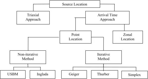
A classification of the source location methods based on the above discussion is presented in Fig. 1 and our discussion will closely follow the logic shown by the flow chart. It has to be emphasized that this classification is developed mainly for the convenience of the discussion and should not be interpreted as a serious effort to classify the source location methods.
The detailed discussion on the location algorithms will be split into two papers. The present paper covers the triaxial sensor method, zonal location technique and two non-iterative algorithms: Inglada method and USBM method. The second paper deals exclusively with the subject of iterative algorithms.
Fig. 1. Classification of AE/MS source location methods.
Source Location Triaxial Approach Arrival Time Approach Point Location Non-iterative Method Iterative Method
Inglada Geiger Thurber Simplex
Zonal Location
3. Triaxial Sensor Approach
The triaxial sensor approach is based on the idea that if the spatial position of a point is known, then the spatial position of any other point can be expressed in terms of its relative distance and azimuth to the known point. The unique advantage of this approach is that the source location can be carried out from a single location. The approach is therefore critical for those deep level applications where long drill holes are required for the sensor installation. The approach has been utilized for various deep level applications, such as rockburst study (Brink and Mountfort, 1984), stability of petroleum reserve site (Albright and Pearson, 1979), and geothermal engineering (Albright and Pearson, 1979; Baria and Batchelor, 1989; Niitsuma et al., 1989).
3.1 Location principle
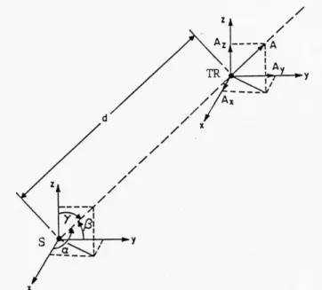
The geometry of the triaxial sensor approach is illustrated in Fig. 2. Here the location of a triaxial sensor, TR, is known. Source S is to be determined in terms of its relative distance, d, and its azimuth (α, β, γ).
Fig. 2. The geometry associated with triaxial sensor approach (After Hardy, 1986). Based on the P- and S-wave arrival times, the relative distance can be expressed as
) ( s p s p s p t t v v v v d − − = (2)
where d is the distance from the source to the sensor, vp and vs are the velocities of P- and S-waves, and tp and ts are the arrival times of P- and S-waves.
The relative azimuth (α, β, γ ) can be determined by the amplitude of the received signals. Assuming that Ax, Ay and Az are the amplitudes of three mutually orthogonal components of the signal. The direction cosines of this signal relative to the sensor are
A A l = x/ m= Ay/A p= Az /A (3) and 2 2 2 z y x A A A A= + + (4)
where l, m and p are the direction cosines of the signal relative to the sensor. The relative azimuth is simply ) ( cos−1 l = α ) ( cos−1 m = β (5) ) ( cos−1 p = γ
Using signal amplitudes to determine the relative azimuth is based on the fact that, for a compressional wave, the first particle motion is in the direction of propagation (Hardy, 2003).
3.2 Least squares solution for azimuth
When there are n sets of observations, such as
i xi i A A l = / , i yi i A A m = / , i = 1, 2, ……, n i zi i A A p = / ,
the best solution defined by the least squares method is:
∑
= = − ∂ ∂ n i i xi A A l l 1 2) 0 ) / ( (∑
= = − ∂ ∂ n i i yi A A m m 1 2) 0 ) / ( (∑
= = − ∂ ∂ n i i zi A A p p 1 2) 0 ) / ( ( .where l, m, and p are the best fit for lis, mis and pis. Solving the above equations, we have
n A A l =
∑
( xi/ i) n A A m=∑
( yi/ i) (6) n A A p=∑
( zi / i) 3.3 DiscussionTriaxial sensor approach is found extremely useful for those deep level applications where borehole drilling is required for the sensor installation. Since borehole drilling is a very expensive operation, it has to be minimized. With the triaxial sensor approach, the required location accuracy may be achieved with a single or few sensors which effectively reduces the request for borehole drillings.
In addition to its cost benefit for deep level applications, there are two technical advantages associated with the triaxial sensor approach. First, it improves the stability of the source location solutions for those outside array events as the approach uses both P- and S- wave arrivals. Second, it allows one to analyze the status of the ground motion at the sensor location, which is critical for studying event magnitude and source mechanism.
The major technical problem associated with the triaxial sensor approach is the stability of the azimuthal angles as amplitudes are much more sensitive to material properties and structures than travel times. A technique that could improve the problem is called hodogram (Doebelin, 1975). With this technique, amplitude data from two components are cross-plotted and an elliptical figure is obtained. The major axis of the ellipse is considered the direction of wave propagation in the plane. Figure 4 shows the hodogram of particle motions detected by two horizontal sensors.
Fig. 3. Hodogram of particle motions detected by two horizontal sensors (after Hardy, 2003).
4. Zonal Source Location
Zonal location is a source location technique that identifies a predefined zone as the event location based on, primarily, the location of the first triggered sensor. It is the simplest form to use arrival times for source location. If the network is relatively dense with a good coverage, the technique offers a quick and reliable idea on the general area where the event took place.
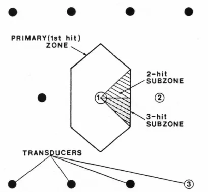
The concept of zonal location and its application to large structures originated from AE studies in material science (Arrington, 1984; Fowler, 1984; Tiede and Eller, 1982; and Hutton and Storpik, 1976). The idea of the zonal location is demonstrated in Figure 4. Here the monitoring region is divided into a number of primary zones, and each zone is associated with a particular station which is the first one to be triggered when the source is located within the area. Based on the locations of the later triggered stations, the primary zone is further divided into smaller ones, such as the second-hit sub-zone and the third-hit sub-zone as illustrated in the figure.
The sub-zones provide the better idea on the relative azimuth position of the source in the primary zone, but offers no improvement in the radial direction. The problem may be overcome by two simple techniques. The first one is to compare the observed arrival time difference between the first and the later triggered stations with the associated theoretical limit. The theoretical limit is the distance between two sensors divided by the velocity. The ratio of the
Fig. 4 The geometry associated with the zonal location method (after Hardy, 2003).
observed arrival time difference to the theoretical limit is an indication of the event location. The larger the ratio, the closer the source to the first triggered station. If the ratio reaches to one, the source is at or behind the first triggered station. If it is zero, the source is on the central line between the two stations, or on the board of the primary zone. The second technique is to use the P- and S-wave arrival time difference to estimate the distance from the first station, which can be done by using Eq. (2).
In comparison with the methods designed for the pin-point location purpose, the zonal location approach has two distinctive advantages. First it does not need to determine the precise ray trace, which is often very difficult when the structure under the study is complicated. It is largely because of this reason that the zonal location becomes one of the primary methods used in the non-destructive testing industry. The other advantage of the method is that it posts no request on the minimum number of stations to be triggered. Lack of the sufficient stations for precise source location is a frequently observed problem. When this is the case, the zonal location becomes the only alternative.
An important assumption made with the zonal location approach is that all stations are triggered by the same wave type, presumably by P-waves. This, however, may not necessarily be the case. In fact, AE systems are often triggered by S-waves instead of P-waves. This is because amplitudes of P-waves are often much lower than that of S-waves, and this phenomenon is shown in Figure 5 by an AE signal recorded by a triaxial sensor.
In addition to the S-wave triggering, experimental conditions may also play an important role. For instance, it was observed by the author in the test of a water-filled tank car that the sensor at the opposite side of the calibrated source was triggered instead of those closer ones on the same side. This is because the water-borne P-wave that triggered the sensor at the opposite side was less attenuated while the metal-borne waves that had supposedly triggered the nearby
Fig. 5. AE signals detected using a triaxial monitoring transducer (after Hardy, 2003). It is understood from the above discussion that the zonal location technique, as any other source location methods, is subject to errors and the causes for the error are not uncommon. Therefore, the solution by the zonal location should not be automatically assumed correct and should be examined if it is possible.
5. Inglada's Method
We now begin our discussion on non-iterative methods. Non-iterative methods are an important category in the family of location algorithms. They are simple and easy to use, and, in fact, the basic ones used by AE practitioners. Inglada’s method and USBM method are considered the representatives in this category and we discuss Inglada’s method first.
5.1 Algorithm
Inglada's method (Inglada, 1928) is a non-iterative, analytical solution of the source location problem defined by Eq. (1). The method is best suited for simple source location problems where the number of sensors used is minimum and a constant velocity model can be assumed.
Inglada method starts with squaring Eq. (1):
2 2 2 2 2 ( ) ( ) ( ) ) (xi −x + yi −y + zi −z =v ti −t (7)
for i = 1, 2, 3, and 4 and then linearizes the system by subtracting the first equation from three remaining ones, which yields:
t f e z c y b x ai + i + i = i + i (8) where 1 x x ai = i − 1 y y bi = i − 1 z z ci = i − )) ( ( 5 . 0 2 1 2 2 2 1 2 R v t t R ei = i − − i − ) ( 1 2 t t v fi = i − and 2 2 2 2 i i i i x y z R = + + 2 1 2 1 2 1 2 1 x y z R = + + for i = 2, 3, and 4.
Three linear equations defined in (8) can be solved for x, y and z in terms of t by using Cramer's rule. The solution is as follows:
D t N M x= 1+ 1 D t N M y = 2 + 2 (9) D t N M z= 3 + 3
where D is the determinant given by
⎥ ⎥ ⎥ ⎦ ⎤ ⎢ ⎢ ⎢ ⎣ ⎡ = 4 4 4 3 3 3 2 2 2 c b a c b a c b a D .
Mj and Nj, for j = 1, 2 3, are also the determinants. They are similar to D, but with the jth column of D replaced by (e2, e3, e4) and (f2, f3, f4), respectively.
Substitute three equations defined in (9) back to one of the equations defined in (7). Since x,
y and z in (9) are all expressed in terms of t, this back substitution yields a second order equation of t with the form
At2 + Bt + C = 0 (10)
where A, B and C are constants.
Eq. (10) is a quadratic function of t and there are two solutions, say, t01 and t02. Substituting
t01 and t02 into Eq. (9), the corresponding solutions are (x01, y01, z01, t01) and (x02, y02, z02, t02), respectively.
5.2 Identifying non feasible solution
the observed arrival time(s). Otherwise, a further check is necessary in order to determine the true source location. This is usually done by substituting the solutions back into the nonlinear system defined in Eq. (1). There is, however, the possibility that both the solutions satisfy those nonlinear equations, which are called multiple solutions. When the problem of multiple solutions is encountered, the arrival time data from an additional sensor is required to identify the true source.
5.3 Multiple solutions
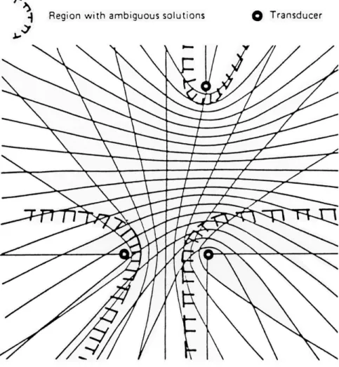
The problem of multiple solutions is not caused by the Inglada’s method. Rather, it is due to the non-linear nature of the location formulas. It can be shown that the problem will occur only when the minimum number of sensors is utilized for location computation (Ge, 1988). Figure 6 illustrates the multiple solutions associated with a 2-dimensional array.
Fig. 6. Distribution of multiple solutions (After Rindorf, 1981)
5.4 Application conditions
Inglada's method is simple and easy to use. In fact, it is probably the simplest algorithm for solving a set of equations defined by Eq. (1). Users however need to be aware of its operational conditions. First, it is understood from the deriving process that the algorithm assumes the same velocity for all stations. This assumption may restrict the meaningful use of the method in many cases and should be validated before its application.
Second, the algorithm uses only a minimum number of sensors that is mathematically required for the pin-point location, that is, the number of equations is equal to the number of unknowns. Because of this requirement, no optimization method can be applied to the algorithm.
From an error control point of view, one should use as many sensors as possible. There are two important reasons. First, the location accuracy is fundamentally determined by the sensor array geometry (Ge, 1988). Using more sensors in general will lead to the better array geometry. Second, the data set is statistically more reliable when more sensors are used. Christy (1982) demonstrated that the algorithm incorporated with the least squares method would yield the better source location accuracy than Inglada method. For these reasons, one should consider to use the algorithms with the optimization capability if the location data is available from sensors that are more than the minimum.
6. The USBM Method
The USBM method is a non-iterative algorithm for the source location problem defined by Eq. (1). It was developed in the early 1970s by the researchers at the United States Bureau of Mines (USBM). The development of this method was part of the Bureau of Mines' effort to make the acoustic emission/microseismic (AE/MS) technique an effective engineering tool for determining the stability of rock structures. The method was first published in 1970 and was further modified in 1972 (Leighton and Blake, 1970; Leighton and Duvall, 1972). Since then it has become the major mine-oriented AE/MS source location method used in North America.
6.1 Algorithm
Let Di represent the distance from the source to the ith transducer,
2 2 2 ( ) ( ) ) (x x y y z z Di = i − + i − + i − (11)
and rewrite Eq. (1) as
) (t t v
Di = i − . (12)
Subtract the first equation from the rest which are all defined by Eq. (12),
)
( 1
1 v t t
D
Di − = i − (13)
where, i = 2, 3, ..., m. Squaring and simplifying the above equation, this yields
1 2 ) ( 2 D d z c y b x a d e d i i i i i i i =− + + − + (14) where i i x x a = 1− i i y y b = 1 − i i z z c = 1− ) (t t1 v di = i − ) ( 2 2 2 2 1 2 1 2 1 i i i i x y z x y z e = + + − + +
The non-linear system defined by (14) can be linearized by subtracting the 2nd equation from the rest of them. This process yields
where ) ( 2 2 2 1 , i i i t a t a f = − ) ( 2 2 2 2 , i i i t b t b f = − ) ( 2 2 2 3 , i i i t c t c f = − i i t t g = 2 − i i i t e t e h = − 2 2 i = 3, 4, …, m. Eq. (15) defines a linear system.
In matrix notation, the linear system defined by Eq. (15) can be written as
Ax = b (16) where ⎥ ⎥ ⎥ ⎦ ⎤ ⎢ ⎢ ⎢ ⎣ ⎡ = 3 , 3 , 3 2 , 2 , 3 1 , 1 , 3 m m m f f f f f f A , ⎥ ⎥ ⎥ ⎦ ⎤ ⎢ ⎢ ⎢ ⎣ ⎡ = z y x x , ⎥ ⎥ ⎥ ⎦ ⎤ ⎢ ⎢ ⎢ ⎣ ⎡ + + = 2 2 3 3 v g h v g h b m m .
6.2 The least squares solution
It is important to note that the USBM method requires the arrival times from at least (n + 1) stations, where n is the number of unknowns. For instance, if there are five stations, A is a 3 by 3 matrix and unknowns, x, y and z, can be solved exactly. If there are arrival times from more than five stations, the source location has to be defined statistically. With the USBM method, the error is conventionally defined as the sum of squares of residuals and the corresponding least squares solution is (Strang, 1980):
ATAx = ATb (17)
or
x = (ATA)-1ATb
The origin of time is not given in x; but it can be obtained by substituting x back into (1).
6.3 Velocity as an unknown
The velocity can be estimated by the USBM method and this can be done by considering v2
as an unknown variable in Eq. (15) and moving giv2 from the right hand side of the equation to the left, such as:
i i i i i x f y f z g w h f,1 + ,2 + ,3 − = (18) where w = v2.
While it is an additional freedom to treat the velocity as an unknown, an extra caution should be exercised to use this feature. The main reason is the errors and uncertainties associated with the arrival time information. If the velocity is treated as an unknown, we have the less chance to isolate the arrival time errors to the places where they occur. Instead, they may be “accommodated” by a false velocity value, creating an even worse situation.
6.4 Discussion
The USBM method is a fairly straight forward algorithm for solving a set of non-linear equations defined by (1). With this method the origin time is eliminated by subtracting the first equation from the rest. The resulting equations are then linearized and form a linear system.
There are two basic conditions to use the USBM algorithm. First the method assumes the same velocity for all stations, and second it requires at least one more equation than the number of unknowns, that is, the condition m≥n + 1 must be satisfied, where m and n denote the number of equations and unknowns, respectively. For instance, we need the arrival time information from at least 5 stations in order to solve a problem of 4 unknowns, such as x, y, z, and t.
The major advantage of the USBM method over the Inglada’s method is that all available arrival time information can be used simultaneously for the source location calculation. This allows the statistic analysis to be carried out, an important approach to improve the location accuracy.
There is another similar algorithm which is called the ISA Mine's method, and readers may refer to Godson and McKavanagh (1980) for details.
7. Conclusions
In terms of the physical data utilized for source location, we have two distinctive approaches: the triaxial sensor approach and the arrival time approach. The importance of the triaxial sensor approach may be viewed from two perspectives. First, the source location can be carried out from a single sensor location, which becomes a particular important advantage when sensor installation is expensive. Second, it provides the data that allows one to characterize the status of stress wave at the point, which is critical for the further study of the source mechanism and source parameters.
The limited use of the triaxial sensor approach is primarily due to the two practical reasons. First, the amplitude data is more susceptible to material structures and properties, and therefore, the method is less stable than the one that uses only arrival times. Second, three single-element sensors with spread locations in general give the much better data for source location than a triaxial sensor. Therefore, the arrival time approach is normally the choice from a cost-benefit point of view unless there are some other special considerations.
Zonal location technique is considered a special case of the arrival time approach since all other methods in this category are for pin-point location purpose. Zonal location technique is simple and easy to use. Users, however, still should pay attention to arrival types. The technique is based on the assumption that all sensors are triggered by the same type of wave. As it was discussed in the paper, this might not be the case.
There are two major branches within the arrival time approach: non-iterative and iterative. The “Δt” algorithms that are conventionally called and used by AE practitioners are non-iterative. Inglada and USBM methods are the representatives in this category. Non-iterative methods are simple and easy to use in that they require little interaction from users. The major difference between these two methods is that Inglada method is limited to the minimum number of sensors while USBM method does not subject to this limitation. A common problem with these two methods is the assumption of a single velocity, which severely restricts their valid applications.
The solution to the problem of the single velocity assumption is to use the iterative methods, which are discussed in the accompanying paper: Analysis of source location algorithms Part II: iterative methods.
Acknowledgments
I am grateful to Dr. Kanji Ono for his encouragement to write my research experience in the area. I thank Dr. R. Hardy for his thorough review and the anonymous reviewer for his comments and suggestions to improve the manuscript.
References
Albright, J. N. and C. F. Pearson (1979). Microseismic monitoring at Byran Mound strategic petroleum reserve, Internal Report, Los Alamos Scientific Laboratory, Los Alamos, March 1979. Albright, J. N. and C. F. Pearson (1982). Acoustic emission as a tool for hydraulic fracture location: experience at the Fenton Hill hot dry rock site, Society Petroleum Engineering Journal, August 1982, 523-530.
Arrington, M., (1984). In-situ acoustic emission monitoring of a selected node in an offshore platform, Proc. 7th International Acoustic Emission Symposium, Sendai, Japan, October 1984, 381-388.
Baria, R. K. and A. S. Batchelor (1989). Induced seismicity during the hydraulic stimulation of a potential hot dry rock geothermal reservoir, Proc. 4th Conference on Acoustic Emission/Microseismic activity in geologic structures and materials, The Pennsylvania State University, October 1985, Trans Tech Publications, Clausthal-Zellerfeld, Germany 327-325.
Doebelin, E. O., (1975). Measurement systems, McGraw-Hill Book Company, New York, 591-593. Christy, J. J., (1982). A comparative study of the “Miner” and least squares location technique as used for the seismic location of trapped coal miners, M.S. Thesis, The Pennsylvania State University, College of Earth and Mineral Sciences, University Park, Pensylvania, August 1982. Fowler, T. J., (1984). Acoustic emission testing of chemical process industry vessels, Proc. 7th International Acoustic Emission Symposium, Sendai, Japan, October 1984, 421-449.
Ge, M., (1988). Optimization of transducer array geometry for acoustic emission/ microsesmic source location, Ph.D. Thesis, The Pennsylvania State University, College of Earth and Mineral Sciences, University Park, Pensylvania, August 1982.
Godson, R. A., M. C. Gridges and B. M. Mckavanagh (1980). A 32-channel rock nomise source location system, Proc. 2nd Conference on Acoustic Emission/Microseismic activity in geologic structures and materials, The Pennsylvania State University, November 1978, Trans Tech Publications, Clausthal-Zellerfeld, Germany 117-161.
Hardy, H. R. (1986). Source location velocity models for AE/MS field studies in geologic materials, Proc. 8th International Acoustic Emission Symposium, Tokyo, Japan, October 1986, Japanese Society for Non-Destructive Testing, Tokyo, 365-388.
Hardy, H. R. (2003). Acoustic emission/microseismic activity, A.A. Balkema, Lisse, Netherlands. Hutton, P. H. and J. R. Skorpik (1976). A simplified approach to continous AE monitoring using digital memory storage, Proc. 3rd International Acoustic Emission Symposium, Tokyo, Japan, September 1976, 152-166.
Inglada, V., (1928). Die berechnung der herdkoordinated eines nahbebens aus den eintrittszeiten der in einingen benachbarten stationen aufgezeichneten P-oder P-wellen, Gerlands Beitrage zur Geophysik 19, 73-98.
Leighton, F. and W. Blake (1970). Rock noise source location techniques, USBM RI 7432.
Leighton, F. and W. I. Duvall (1972). A least squares method for improving rock noise source location techniques, USBM RI 7626.
Niitsuma, H., K. Nakatsuka, N. Chubachi, H. Yokoyama, and M. Takanohashi (1989). Downhole AE measurement of a geothermal reservoir and its application to reservoir control, Proc. 4th Conference on Acoustic Emission/Microseismic activity in geologic structures and materials, The Pennsylvania State University, October 1985, Trans Tech Publications, Clausthal-Zellerfeld, Germany 327-325.
Rindorf, H. J., (1981). Acoustic emission source location, Bruel & Kjaer, Technical Review, No. 2. Strang, G. (1980). Linear algerbra and its applications, Academic Press Inc., New York, New York. Tiede, D. A. and E. E. Eller (1982). Sources of error in AE location calculations, Proc. 6th International Acoustic Emission Symposium, Susono, Japan, October/November 1982, 155-164.