TR
OP
E
R
HC
RA
ES
E
R
PAI
D
I
MULTI-LAYER BOOSTING FOR PATTERN
RECOGNITION
Francois Fleuret
Idiap-RR-76-2008
DECEMBER 2008
Multi-Layer Boosting for Pattern Recognition
Fran¸cois Fleuret
August 26, 2008
Abstract
We extend the standard boosting procedure to train a two-layer clas-sifier dedicated to handwritten character recognition. The scheme we propose relies on a hidden layer which extracts feature vectors on a fixed number of points of interest, and an output layer which combines those feature vectors and the point of interest locations into a final classification decision.
Our main contribution is to show that the classical AdaBoost proce-dure can be extended to train such a multi-layered structure by propa-gating the error through the output layer. Such an extension allows for the selection of optimal weak learners by minimizing a weighted error, in both the output layer and the hidden layer. We provide experimental results on the MNIST database and compare to a classical unsupervised EM-based feature extraction.
1
Introduction
Most of the efficient image classification methods combine two levels of mod-elling. At a lower level, feature extraction recodes the input so that local appear-ance of the image is captured with invariappear-ance to translation. At an upper level the features captured locally are combined with a global configuration model. These two steps are present in a form or another in two-layer convolutional net-works [9, 3], certain decision trees for digit recognition [1], constellations [8, 4] or Bayesian models.
We propose in this paper to extend boosting to train the two levels of such a model jointly. Since boosting can be seen as a functional gradient descent, it can be naturally extended to train a multi-layer classifier, each layer of which being a linear combination of simple functionals taking as input the responses of the functionals from the previous layer. This is similar to the extension of gradient descent from a one-layer to a multi-layer perceptron.
The classifier we describe in this paper to illustrate this idea is composed of three stages. The first one is ad hoc and tags points of interest in the image. The second extracts at each of these points a feature vector which is a function of its neighborhood in the image. The third layer combines both the point of interest locations and the feature vectors to obtain a final response. The functionals
doing the feature extraction and the functionals doing the final decision are linear combinations of simple weak learners, selected iteratively in a boosting-like manner to minimize an empirical weighted error rate.
2
Multi-Layer Boosting
2.1
Classical AdaBoost
Boosting [2] was proposed initially as a way to improve the power of a family of classifiers by combining a few of them linearly. The usual way to understand it intuitively is as a technique to increasingly put the emphasis on problematic training examples, so that classifiers built successively are more and more ded-icated to challenging samples, thus reducing the global error rate. However, boosting can also be seen as a functional gradient descent where the resulting mapping is obtained by constructing iteratively a linear combination of simple functionals to reduce a loss in a greedy fashion.
Precisely, letX denote the signal space and by
- {(x1, y1), . . . ,(xN, yN)} ∈(X × {−1,+1})N a training set,
- ˜g1, . . . ,g˜B,∀b,g˜b:X → {−1,1} a set of weak learners,
- ∀t≤T, gt=
Pt
s=1βs˜gbs the mapping obtained aftert steps of boosting.
The role of the AdaBoost procedure is to select the sequence of indexes
b1, . . . , bT and weightsβ1, . . . , βT so that the sign ofgT(xn) is a good predictor
of the classyn. As said above, it can be seen as a functional gradient descent
[6]: each added weighted weak learner is as a small step in the vector space of
functionals, chosen so that an exponential lossLis minimized.
More precisely at any step, given the functionalgt:X →Rbuilt so far and
an exponential loss functionL(g) =Pnexp(−yng(xn)), the algorithm chooses
the weak learner ˜gb(t+1) maximizing
¯ ¯ ¯ ¯ ¯ ∂ L(gt+βg˜) ∂ β ¯ ¯ ¯ ¯ β=0 ¯ ¯ ¯ ¯ ¯= ¯ ¯ ¯ ¯ ¯ X n −yn˜g(xn) exp(−yngt(xn)) ¯ ¯ ¯ ¯ ¯
which corresponds to choosing the direction minimizing the loss the most locally.
Given that weak learner,βt+1 is uniquely defined as
βt+1= arg min
β
L(gt +β˜gb(t+1))
which corresponds to the line search in gradient descent, and has an analytical form in the case of the exponential loss we consider here.
Thus, this is afunctional generalizationof the usual gradient descent. The
only restriction is that not all directions in the space of functions are available, but only the ones corresponding to the weak learners.
2.2
Extension to compositions of mappings
We consider now a slightly more complex situation where the classification rule is a composition of sums of weak-learners. In this settings, a first combination
of weak learners maps the input spaceX intoRQ, and a second combination of
weak learners mapsRQ into{−1,1}.
We introduce the following notations
- {(x1, y1), . . . ,(xN, yN)} ∈(X × {−1,+1})N a training set,
- ˜f1, . . . ,f˜A,∀a,f˜a:X → {−1,1}Q a set of weak learners for the
interme-diate recoding,
- ∀t≤T, ft=
Pt
s=1αsf˜as the mapping for the intermediate recoding built
aftert steps of boosting,
- ˜g1, . . . ,g˜B,∀b,g˜b:X ×RQ→ {−1, 1}a set of weak learners for the output
mapping,
- ∀t≤T, gt=
P
s≤tβs˜gbs the output mapping built aftert steps of
boost-ing.
Thus, when the training is over, given a signal x, the predicted class
cor-responds to the sign ofgT(x, fT(x)). We can transpose directly the AdaBoost
training rule presented above, which leads to choose theat, αt,btand βt+1 to
minimize
L(gt, ft) =
X
n
exp(−yngt(xn, ft(xn)))
the choice of bt+1 is done with a strict AdaBoost rule, that is by choosing for
˜ gt+1 the ˜g minimizing ∂ L(gt+β˜g, ft) ∂ β ¯ ¯ ¯ ¯ β=0 =X n −yn˜g(xn, ft(xn)) exp(−yngt(xn, ft(xn)))
which is a weighted error rate of ˜g. The choice ofβt is obtained by line
mini-mization which has a closed form, as usual.
The choice of at+1 is however slightly more complex. We again apply the
minimization of the local derivative, that is we want to pick for ˜fat+1 the ˜f
minimizing ∂ L(gt, ft+αf˜) ∂ α ¯ ¯ ¯ ¯ ¯ α=0 =X n ∂ exp(−yngt(xn, ft(xn) +αf˜(xn))) ∂ α ¯ ¯ ¯ ¯ ¯ α=0 =X n −yn ∂ gt(xn, ft(xn) +α ˜ f(xn)) ∂ α ¯ ¯ ¯ ¯ ¯ α=0 exp(−yngt(xn, ft(xn))) =X n X q −ynf˜q(xn)∇qgt(xn, ft(xn)) exp(−yngt(xn, ft(xn)))
1 2 3
f
g
K(u , v )
K 1 1(u , v )
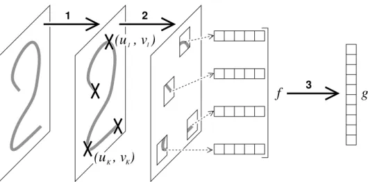
Figure 1: The classification is composed of three steps: (1) on the input image
Ia fixed numberKof points of interest (u1, v1), . . . ,(uK, vK) are tagged on the
maxima of a difference of Gaussians, (2) a feature vector of sizeDis computed
for each of these points of interest, as a function of the ∆×∆ neighborhood of
each points, resulting in a vectorf(I) of dimension D K, (3) one response gc
is computed for each of theC classes as a function of both the locations of the
points of interest and the feature vectors.
where ˜fq denotes theq-th component of ˜f, and∇qg
t(x) theq-th component of
the gradient of ˜ginx. Hence, the choice of the weak learners for the intermediate
recoding is also the minimization of a weighted error. The coefficientαt+1 is
chosen with a line-search, which has to be done numerically with a standard bracketing procedure, since no analytical form can be derived anymore.
3
Application to character recognition
3.1
Recognition
Our predictor is very close in spirit to a convolutional multi-layer perceptron [9, 3] and consists of a hidden layer extracting the local appearance of the pattern to classify at a few points selected by a difference-of-Gaussian operator [5], and of a second layer combining these local prediction with global geometrical properties to obtain a classification.
More precisely, as described on Figure 1, given an image of size 32×32, the
algorithm is:
1. Select in the 32×32 images a small number K(= 10) of point using the
difference of Gaussian maximization criterion [5]. Let (u1, v1), . . . ,(uK, vK)∈ {0, . . . ,31}2K
denote their coordinates andxthe pair composed of the image itself and the coordinates of these points.
2. For every selected point k, extract a subimage I(uk, vk) of resolution
∆×∆ (with ∆ = 11) centered on (uk, vk) and compute a feature
vec-tor (ψ1(I(uk, vk)), . . . , ψD(I(uk, vk))) withD= 32, and where the ψd are
linear combinations of thresholded Haar wavelets.
At the end of that step, the image has been recoded into a list ofKpoints,
each one being characterized by its two coordinates (uk, vk) in the image
plan and a vector of D features. Let f(x) denote the resulting vector of
dimensionD K.
3. Compute as many scores as there are classes (g1(x, f(x)), . . . , gC(x, f(x)))
and apply a winner-take-all rule to make a hard decision.
3.2
Training
The training algorithm consists of building iteratively and jointly the ψd as
sums of thresholded Haar wavelets [7] and the g1, . . . , gC as sums of smooth
disjunctions of the ψd. To fit this algorithm in the framework described in
§2.2, we consider the signalxto be both the input image in gray levels and the
coordinates of the points of interest (u1, v1), . . . ,(uK, vK), thusX = [0,1]32×32×
{0, . . . ,31}2K
The number of intermediate features is Q =D K, that is as many as the
number of features per point of interest, time the number of points of interest.
Thus, the resulting mappingfT we wish to obtain at the end of the training has
the following form
fT(x) = ψ1(I(u1, v1)), . . . , ψD(I(u1, v1)) | {z } Dfeatures on (u1,v1) , ψ1(I(u2, v2)), . . . , ψD(I(u2, v2)) | {z } Dfeatures on (u2,v2) , . . .
and a weak learner ˜f is defined by an indexd(corresponding to theψd we are
implicitely modifying), a Haar waveleth[7] and a thresholdτ, and is equal to
˜ f(x) = 0, . . . ,0, σ(h(I(u1, v1))−τ),0, . . . ,0 | {z } Dfeatures on (u1,v1) ,0, . . . ,0, σ(h(I(u2, v2))−τ),0, . . . ,0 | {z } Dfeatures on (u2,v2) , . . .
whereσis the heavyside function equal to−1 on R− and +1 onR+.
Every weak learner ˜g is defined by an indexdand a rectangular areaRand
is a smooth maximum of the responses ofψd on the points (uk, vk) localized in
R: ˜ g(I) = 1 − 2 1 + X (uk,vk)∈R exp (ψd(I(uk, vk))) −1 .
Such an expression varies between −1 and 1 and roughly increases with the
maximum over the value ofψd on points contained in the rectangle R.
We initially break the symmetry between features by populating all the ψd
with one wavelet picked at random. The training is done by applying the
gener-alized AdaBoost procedure described in§2.2, with the optimization performed
at each iteration by sampling at random 1,000 weak learners and keeping the
optimal one according to the current weightings.
In the following, we introduceξc
t =gc(xt) and ζt,kd =ψd(It(utk, vtk)). Also,
for the sake of clarityLdenotes either the loss as a function of the responses in
the hidden layer or in the output layer.
One learning step can be summarized as follow:
∀t, c,ξ˙c t ← ∂ξ∂Lc t ∀t, k, d,ζ˙d t,k ← ∂ζ∂Ld t,k = P c∂ξ∂Lc t ∂ξc t ∂ζd t,k ford= 1. . . D do (h∗, τ∗)←arg max h,τ ¯ ¯ ¯Pt,k ζ˙t,kd σ(h(It(utk, vtk))−τ) ¯ ¯ ¯ α∗←arg min αL(ψ1, . . . , ψd+α σ(h∗−τ), . . . , ψD) ψd←ψd+α∗σ(h∗−τ) end for forc= 1. . . C do ˜ g∗←arg max ˜ g ¯ ¯ ¯Pt,k ξ˙ctg˜(xt) ¯ ¯ ¯ β∗←arg min βL(g1, . . . , gc+βg˜∗, . . . , gC) gc←gc+β∗g˜∗ end for
4
Results
We compare the performance of such a multi-layer boosting approach to a more classical unsupervised clustering to select the features. Also, we study the in-fluence of the number of wavelets in the feature coding on the final performance of the classifier both in term of exponential loss reduction during training and in term of test error rates.
4.1
Baseline method
To measure the improvement of performance due to the joint learning, we use for baseline a very similar two-layer classifier. As for our approach, the hidden
layer is composed ofDfeature extractors, the responses of which are combined
into the output layer through disjunctions over rectangular areas. The training algorithm for that output layer is the same as for our approach, and boils down
to a classical AdaBoost procedure (see the choice of thebtandβtcoefficients in
§2.2, page 3).
However, the hidden layer for this baseline is trained in a non-supervised manner. This is done by fitting a mixture of Gaussian densities to the training
data with a standard EM procedure, hence learning a family of D centroids.
By taking into account the variance of classes, such a procedure is slightly more
accurate thank-mean, used with success for building such code-books of patches
[8].
Hence, we first build a training set containing all the ∆×∆ images centered
on the points of interest in the training images. We initialize the EM procedure
by pickingD samples in this set as the initial average samples the classes, and
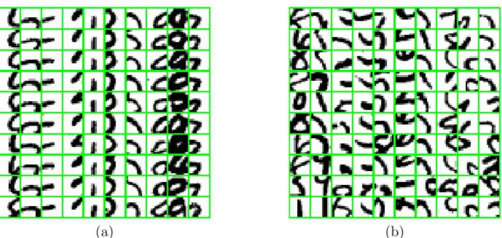
associating each sample of the complete set to the cluster of closest average. From this initialization we apply the classical EM updating rule for mixtures of Gaussians: The expectation and variance of each cluster and the probability of each sample to belong to each class are estimated alternatively. To deal with the high dimension of the space we force the covariance matrix to be proportional to the identity. Figure 5 (a) shows for 10 classes the 10 samples responding the most.
Given an imageI of resolution ∆×∆, we can compute a feature vector of
dimensionD by first computing the distances to the D centroids chosen with
the learning procedure described above, and then by thresholding each of these
D distance. The choice of thresholds that gave the best results on the test set
was the median of each distance on the training examples. Hence, during test there are always roughly half of the features below threshold and half of the feature above threshold.
This baseline has all the strengths of the new method we propose except that it lacks the joint training of the hidden layer: The features encoded in the hidden layer are here trained separately in a non-supervised way.
4.2
Influence of the number of wavelets on the training
error
Our first series of experiments tests the performance of the classifier trained
with N = 10,000 samples, with T = 100 weak learners for each class in the
output layer and various numbers of wavelets in the hidden layer.
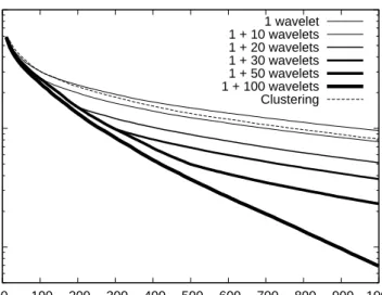
Figure 2 shows the evolution of the exponential loss as a function of the number of weak learners in the output layer, and Figure 3 as a function of the number of wavelets in the hidden layer, for a fixed number of weak learners in the output layer.
103 104 105
0 100 200 300 400 500 600 700 800 900 1000
Training exponential loss
Number of weak learners
1 wavelet 1 + 10 wavelets 1 + 20 wavelets 1 + 30 wavelets 1 + 50 wavelets 1 + 100 wavelets Clustering
Figure 2: Exponential loss as a function of the total number of weak learners in the output layer when the wavelets in the hidden layer are added from the first step of learning.
Since we equalize the number of clusters between the baseline and the multi-layer boosting, there are no equivalent “capacity parameter” for the former sim-ilar to the number of wavelets for the latter. Hence results are always computed after convergence of EM for the baseline.
As expected, the more wavelets in the hidden layer, the more the loss is reduced. Interestingly, 10 wavelets already outperforms the unsupervised EM clustering and as shown on Figure 4 the test error rate does not improve when adding more than 50 wavelets.
4.3
Testing error rates
Finally, to compare this approach to the state of the art, we have computed the test error rate with the classifiers used in the experiments presented above,
which is built with only 10,000 samples and 100 weak learners in each of theC
functional of the output layers, and also with a classifier trained with the full
MNIST database (60,000 samples) which combines 1,000 weak learners in the
output layer and 50 wavelets per feature in the hidden layer.
In both case, we improve the classification by trying 3 different rotations
in the image plan (−π
20, 0 and +20π) to account for the tilt of the character
and averaging the responses of the output layer over the three rounds. The error rates of the classifiers combining only 100 weak learners are given vs. the number of features on Figure 4. The error rate with the classifier trained on the
0 2000 4000 6000 8000 10000 12000 0 20 40 60 80 100
Training exponential loss
Number of wavelets
Clustering MLB
Figure 3: Exponential loss during training as a function of the number of Haar wavelets used in the hidden layer for the Multi-Layer Boosting (MLB) with 100 weak learners per class in the output layer.
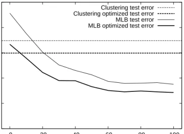
0 2 4 6 8 10 0 20 40 60 80 100 Test error (%) Number of wavelets
Clustering test error Clustering optimized test error MLB test error MLB optimized test error
Figure 4: Test error rates with and without pose optimization as a function of the number of Haar wavelets per feature in the hidden layer. Not shown here is
the error rate of 1.46% with 1,000 weak learners in the output layer, 50 wavelets
(a) (b)
Figure 5: These figure show for each of theD= 32 feature component the eight
∆×∆ subimages with the highest score. Figure (a) corresponds to the EM
clustering and (b) to the multi-layer boosting with 100 wavelets. As observed for multi-layer perceptrons, the features obtained by supervised learning are less consistent geometrically than those learnt by unsupervised learning.
5
Conclusion
We have demonstrated how boosting can be extended to a multi-layer setting. The output functionals are trained with a classical AdaBoost while the inner layer is trained by first propagating the derivative of the loss function through the output layer and then using an AdaBoost-like procedure.
Such an architecture is very close to a multi-layer perceptron (MLP). Still,
it retains all thegoodproperties of boosting, mainly the ability to combine
het-erogeneous weak learners into a unified scheme. Compared to a MLP, the price to pay is computational: since the constructed classifiers do not live anymore in
Rn as MLPs do, the computational cost increases with the number of combined
weak learners.
The computational cost for test is not too high and remains linear with the
number of weak learners, as usual for boosted classifiers. That isO(N1+N2)
whereN1is the number of weak learners in the hidden layer andN2the number
of weak learners in the output layer. On the contrary, the asymptotic training cost increases: since the responses of the output layer weak learners change when the hidden layer is modified, they have to be recomputed at each learning step. Finally, if all the weak learners in the hidden layer are added from the first step,
the learning cost turns to beO(N2
1+N2). However experiments showed that a
few tens of features in theψds are sufficient to reach the maximum performance
(see Figure 4), which means that this asymptotic cost is not a real issue. This study demonstrates that multi-layer boosting is doable and provides the expected improvement due to learning jointly the local and the global model of
the patterns to classify. Our future work will be focused on refining the weak learners combined in the output layer to imbed invariance to translation or local deformations at reasonable cost.
6
Acknowledgments
This work was supported by the Swiss National Science Foundation under the National Centre of Competence in Research (NCCR) on ”Interactive Multi-modal Information Management (IM2).
References
[1] Y. Amit, D. Geman, and K. Wilder. Joint induction of shape features
and tree classifiers. IEEE Transactions on Pattern Analysis and Machine
Intelligence, 19(11):1300–1305, november 1997.
[2] Y. Freund and R. E. Schapire. A short introduction to boosting.Journal of
Japanese Society for Artificial Intelligence, 14(5):771–780, 1999.
[3] Y. LeCun and Y. Bengio. Word-level training of a handwritten word
recog-nizer based on convolutional neural networks. In IAPR, editor,Proceedings
of the International Conference on Pattern Recognition, volume II, pages 88–92, Jerusalem, October 1994. IEEE.
[4] F. Li, R. Fergus, and P. Perona. A Bayesian approach to unsupervised
one-shot learning of object categories. In Proceedings of the International
Conference on Computer Vision, volume 2, page 1134, 2003.
[5] D. G. Lowe. Object recognition from local scale-invariant features. In
Pro-ceedings of the International Conference on Computer Vision, pages 1150– 1157, 1999.
[6] L. Mason, J. Baxter, P. Bartlett, and M. Frean. Boosting algorithms as
gradient descent. InNeural Information Processing Systems, pages 512–518.
MIT Press, 2000.
[7] C. P. Papageorgiou, M. Oren, and T. Poggio. A general framework for
ob-ject detection. InProceedings of the International Conference on Computer
Vision, volume 2, pages 555–562, 1998.
[8] M. Weber, M. Welling, and P. Perona. Unsupervised learning of models
for recognition. In Proceedings of the European Conference on Computer
Vision, pages 18–32, 2000.
[9] Q. Z. Wu, Y. LeCun, L. D. Jackel, and B. S. Jeng. On-line recognition of limited vocabulary chinese character using multiple convolutional neural
networks. In Proceedings of the 1993 IEEE International Symposium on