AVR32723: Sensor Field Oriented Control for Brushless DC motors with AT32UC3B bit Microcontrollers. Application Note. Features.

AVR32723: Sensor Field Oriented Control for

Brushless DC motors with AT32UC3B0256

Features

• Standalone Space Vector Modulation library for AVR®32 UC3 microcontroller.

• Park and Clarke mathematical transformation library for AVR32 UC3 microcontroller.

• Theory of Field Oriented Control.

• PC application for real time motor remote control and display of regulated variables.

1 Introduction

This application note delivers an implementation of Sensor Field Oriented Control algorithm for brushless DC motor on Atmel® AVR32 UC3B microcontrollers.

This software includes standalone libraries for all mathematical transformations required by the algorithm.

For more information about the AVR32 architecture, please refer to the appropriate documents available from http://www.atmel.com/avr32.

2 Requirements

The software provided with this application note requires several components:

• A computer running Microsoft® Windows® 2000/XP/Vista® or Linux®

• AVR32Studio and the GNU toolchain (GCC) or IAR Embedded Workbench® for AVR32 compiler.

• A JTAGICE mkII or AVROne! debugger

32-bit

Microcontrollers

Application Note

AVR32723

3 Theory of Operation

3.1 Overview

As continuity in the energy efficiency process, the increase of capability of microcontrollers allows to implement complex algorithm as Field Oriented Control methodology which allows to:

• Reduce power consumption (less power loss) of electrical motor driving.

• Provide smoother and more accurate motor control than sinusoidal command with hall feedback.

• Optimize motor choice (torque): find the best alternative between dimension and power.

But this algorithm requires more complex computation and requires more CPU bandwidth than standard algorithms.

Moreover, this command strategy fits with some brushless DC motors with dynamical load changes due to reduction of response time. It allows regulating torque and speed at the same time.

3.2 Block Diagram

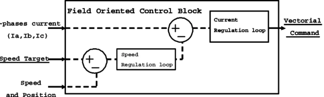
The following block diagram describes the principle of the algorithm. Indeed, it is based on:

• A vectorial command for 3-phases Brushless DC Motors.

• A periodic current sampling of the 3 shunts located on these 3-phases.

• 2 encapsulated regulation loops: one for the current (torque and power loss) and another for the speed.

Figure 3-1.Block Diagram

3-phases current (Ia,Ib,Ic)

Speed and Position Speed Target

Field Oriented Control Block

Vectorial Command Speed Regulation loop Current Regulation loop 3-phases current (Ia,Ib,Ic) Speed and Position Speed Target

Field Oriented Control Block

Vectorial Command Speed Regulation loop Current Regulation loop

Field Oriented Control Block

Vectorial Command Speed Regulation loop Current Regulation loop

AVR32723

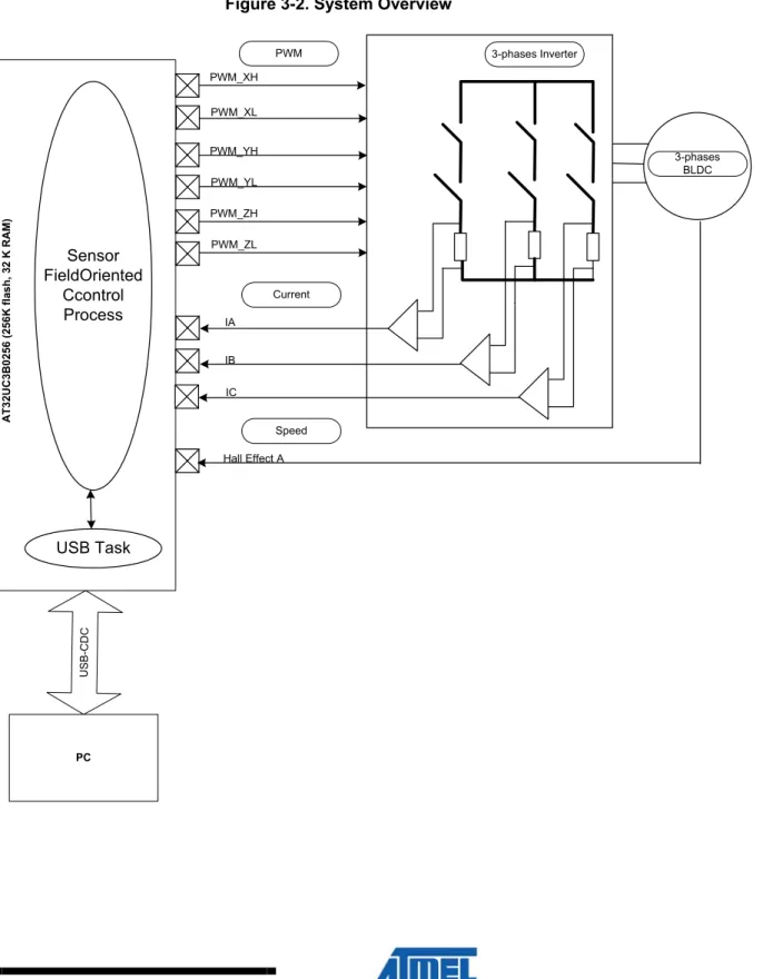
3.3 System Overview

As shown Figure 3-2, the 3-phases current are measured and one Hall Effect feedback is used to compute field oriented control algorithm.

Figure 3-2. System Overview

AT3 2UC3B0 25 6 ( 256 K fl as h, 3 2 K RAM ) U S B -C D C PC PWM Current Speed 3-phases Inverter 3-phases BLDC PWM_XH PWM_XL PWM_YH PWM_YL PWM_ZH PWM_ZL IA IB IC Hall Effect A Sensor FieldOriented Ccontrol Process USB Task

AVR32723

The USB connection is used through a PC application for real time motor remote control and display of regulated variables. This data monitor displays feedback control remotely. This GUI provides:

- 3 graphs and 1 cursor display. - 4 inputs control.

The purpose is to be able to connect to the application without disturbing the behavior of the application. The application offers the following features:

- Implements vector control of a Brushless DC motor. - Speed range from 400 rpm to 2000 rpm.1

- With a 100 µsec control loop, the CPU is used at 35% by the Sensor Field

Oriented Control Process at 42MHz.

- Display in real time the current and speed measured. - Control of speed in real time.

AVR32723

4 Motor Control Theory

4.1 General Model.

The mathematical model in a constant domain linked to the stator is linked to differential equation with constant coefficients defining the motor behavior.

Applying the Lenz-Faraday model, we have:

[ ] [ ] [ ]

abc abc abc

dt

d

I

R

V

=

+

Φ

With:

[ ]

⎥

⎥

⎥

⎦

⎤

⎢

⎢

⎢

⎣

⎡

=

c b a abc

v

v

v

V

,

[ ]

⎥

⎥

⎥

⎦

⎤

⎢

⎢

⎢

⎣

⎡

=

c abc

i

i

i

I

b a and

[ ]

⎥

⎥

⎥

⎦

⎤

⎢

⎢

⎢

⎣

⎡

Φ

Φ

Φ

=

Φ

c b a abc

R is the statoric resistance,

[

]

t c b

a

v

v

v

are the statoric voltages,

[

]

t

c b

a

i

i

i

are

the statoric current and

[

]

t

c b

a

Φ

Φ

Φ

are the global fields in the statoric solenoid.

[ ] [ ][ ] [ ]

Φ

abc

=

L

I

abc

+

Φ

sf We can write :

Ls (constant) is the inductance in a statoric gyres.

M (constant) is the mutual inductance between the 2 statoric gyres θ is the electrical position of the rotor (θ= θélec)

Фsf is the max value (constant) of the flux create by the permanents magnet through the statoric gyres.

⎥

⎥

⎥

⎥

⎥

⎥

⎦

⎤

⎢

⎢

⎢

⎢

⎢

⎢

⎣

⎡

+

Φ

−

Φ

Φ

+

⎥

⎥

⎥

⎦

⎤

⎢

⎢

⎢

⎣

⎡

⎥

⎥

⎥

⎦

⎤

⎢

⎢

⎢

⎣

⎡

+

⎥

⎥

⎥

⎦

⎤

⎢

⎢

⎢

⎣

⎡

=

⎥

⎥

⎥

⎦

⎤

⎢

⎢

⎢

⎣

⎡

)

3

2

cos(

)

3

2

cos(

)

cos(

π

θ

π

θ

θ

sf sf sf c b a c b a c b a

dt

d

i

i

i

Ls

M

M

M

Ls

M

M

M

Ls

dt

d

i

i

i

R

v

v

v

In order to simplify the mathematical resolution of this system, some mathematical transformations are used.

Using the Park P1(θ), the instantaneous power is kept and it allows to have a mathematical expression of the torque still acceptable for the real motor.

[

]

⎥

⎥

⎥

⎥

⎥

⎥

⎦

⎤

⎢

⎢

⎢

⎢

⎢

⎢

⎣

⎡

+

Φ

−

Φ

Φ

+

⎥

⎥

⎥

⎦

⎤

⎢

⎢

⎢

⎣

⎡

⎥

⎥

⎥

⎦

⎤

⎢

⎢

⎢

⎣

⎡

=

Φ

)

3

2

cos(

)

3

2

cos(

)

cos(

π

θ

π

θ

θ

sf sf sf c b a abc

i

i

i

Ls

M

M

M

Ls

M

M

M

Ls

AVR32723

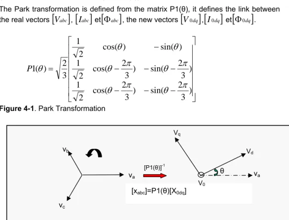
Using the Park inverse transformation, it is possible to return to the values space from regulated values and generate commands.

4.1.1 Park Transformation (P1(θ)) and Clarke Transformation (inv P-1(θ))2.

The Park transformation is defined from the matrix P1(θ), it defines the link between the real vectors

[ ]

V

abc ,

[ ]

I

abc et

[ ]

Φ

abc , the new vectors

[ ]

V

0dq ,

[ ]

I

0dq et

[

Φ

0dq

]

.

⎥

⎥

⎥

⎥

⎥

⎥

⎦

⎤

⎢

⎢

⎢

⎢

⎢

⎢

⎣

⎡

−

−

−

−

−

−

−

=

)

3

2

sin(

)

3

2

cos(

2

1

)

3

2

sin(

)

3

2

cos(

2

1

)

sin(

)

cos(

2

1

3

2

)

(

1

π

θ

π

θ

π

θ

π

θ

θ

θ

θ

P

Figure 4-1. Park Transformation

With V0 =0V, I0 =0A and Φ0 =0Wb, the normalized Park transformation is the addition the Concordia Transformation T32 and the rotating matrix p(θ) :

⎥

⎥

⎥

⎥

⎥

⎥

⎥

⎦

⎤

⎢

⎢

⎢

⎢

⎢

⎢

⎢

⎣

⎡

−

+

−

−

+

=

2

3

2

3

2

2

2

2

0

2

3

1

32

T

⎥

⎦

⎤

⎢

⎣

⎡

−

=

θ

θ

θ

θ

θ

cos

sin

sin

cos

)

(

p

Figure 4-2. 3D to 2D Transformation

2 _{The Park and Clarke transformations are implemented as a software library} component in the software package associated with this application note. See also section 5. [xabc]=P1(θ)[X0dq] va vb vc [P1(θ)]-1 va V0 Vd Vq θ T32t xa xb xc xα xβ P(-θ) Xd Xq

AVR32723

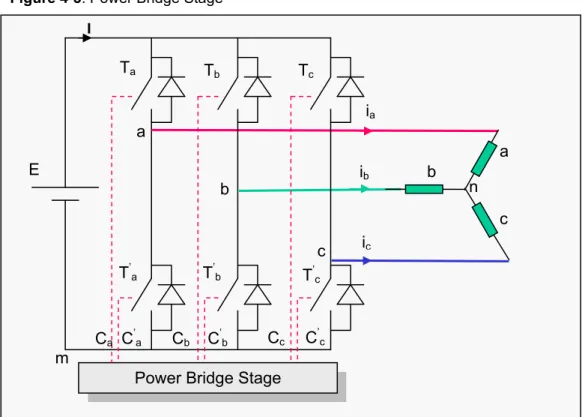
4.2 Power Bridge Command.

The power bridge stage is here to power the BLDC motor with alternatives voltages from a continuous source. This bridge allows modulating frequency and amplitude.

Figure 4-3. Power Bridge Stage

Figure II-1 Onduleur de tension triphasé.

The logical signals Ca, C’a, Cb, C’b, Cc and C’c are command signals for the power bridge.

The output voltages are given from the ground ‘m’ of source generator and from the

virtual neutral point ‘n’ of BLDC motor.

⎥

⎥

⎥

⎦

⎤

⎢

⎢

⎢

⎣

⎡

=

⎥

⎥

⎥

⎦

⎤

⎢

⎢

⎢

⎣

⎡

c b a cm bm am

C

C

C

E

V

V

V

(II-1) nm cn cm nm bn bm nm an am

V

V

V

V

V

V

V

V

V

+

=

+

=

+

=

For an equilibrated load:

V

an

+

V

bn

+

V

cn

=

0

V, so :

V

nm

=

(

V

am

+

V

bm

+

V

cm

)

3

1

. In that way, we have:

⎥

⎥

⎥

⎦

⎤

⎢

⎢

⎢

⎣

⎡

⎥

⎥

⎥

⎦

⎤

⎢

⎢

⎢

⎣

⎡

−

−

−

−

−

−

=

⎥

⎥

⎥

⎦

⎤

⎢

⎢

⎢

⎣

⎡

⎥

⎥

⎥

⎦

⎤

⎢

⎢

⎢

⎣

⎡

−

−

−

−

−

−

=

⎥

⎥

⎥

⎦

⎤

⎢

⎢

⎢

⎣

⎡

c b a cm bm am cn bn an

C

C

C

E

V

V

V

V

V

V

2

1

1

1

2

1

1

1

2

3

2

1

1

1

2

1

1

1

2

3

1

Power Bridge Stage m E Ta a b c ia ib ic a b c n I Tb Tc T’ a T’b T’_c Ca C’a Cb C’b Cc C’c

AVR32723

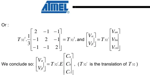
Or :

.

2

1

1

1

2

1

1

1

2

3

1

.

32 32t

T

t

T

=

⎥

⎥

⎥

⎦

⎤

⎢

⎢

⎢

⎣

⎡

−

−

−

−

−

−

and

⎥

⎥

⎥

⎦

⎤

⎢

⎢

⎢

⎣

⎡

=

⎥

⎦

⎤

⎢

⎣

⎡

cn bn an

V

V

V

T

V

V

_t 32 β α We conclude so:

⎥

⎥

⎥

⎦

⎤

⎢

⎢

⎢

⎣

⎡

=

⎥

⎦

⎤

⎢

⎣

⎡

c b a

C

C

C

E

T

V

V

_t

.

32 β α , ( t

T

32 is the translation of

T

32)

The following table gives the voltage values in the spaces (

α

,

β

) and (a, b, c).

Table 4-2. Voltage Values in the spaces (

α

,

β

) and (a, b, c)

We show that all vectors components (Vα, Vβ) are with modules

2

3

E

and are located in the regular hexagon.

Figure 4-4. Space Vector values in the regular hexagon.

Ca Cb Cc Vα Vβ Van Vbn Vcn Vector 0 0 0 V0 1 0 0 V1 1 1 0 V2 0 1 0 V3 0 1 1 V4 0 0 1 V5 1 0 1 V6 1 1 1 V7 E 3 0 0 0 2 -1 -1 1 1 -2 -1 2 -1 -2 1 1 -1 -1 2 1 -2 1 0 0 0 E 2 3 0 0 1 0 1 2 3 2 √ 1 2 3 2 √ -1 0 1 2 3 2 √ 1 2 3 2 √ 0 0 Vβ

1

3

4

5

6

Vα V1 V2 V3 V4 V5 V6 (1, 0, 0) (1, 1, 0) (0, 1, 0) (0, 1, 1) (0, 0, 1) (1, 0, 1) (0, 0, (1, 1,

2

2 3

AVR32723

4.2.1 Space Vector PWM.3

The vectorial modulation uses directly the signal for the Concordia transformation. It supposes that a regulation loop is ever implemented for the generation of Vα and Vβ

components.

As stated below, at a instantaneous point, the power bridge is able to generate only 8 voltages (Vi, i = 0,…,7) in the space of transformation Concordia (Vα , Vβ) with two

components equal to 0 and 6 with the module equal to

E

2

3

and the angle to

( )

π

3

(

i

−

1

)

. Two successive vectors, called Vi and Vi+1 defined a sector i (Figure

4-4) with I from the interval [I, VI].

⎥

⎦

⎤

⎢

⎣

⎡

⎥

⎦

⎤

⎢

⎣

⎡

⎭

⎬

⎫

⎩

⎨

⎧

−

=

⎥

⎥

⎥

⎥

⎦

⎤

⎢

⎢

⎢

⎢

⎣

⎡

⎭

⎬

⎫

⎩

⎨

⎧

−

⎭

⎬

⎫

⎩

⎨

⎧

−

=

⎟⎟

⎠

⎞

⎜⎜

⎝

⎛

=

0

1

)

1

(

3

3

2

)

1

(

3

sin

)

1

(

3

cos

3

2

i

p

E

i

i

E

V

V

V

i i

π

π

π

β α

The power stage is only able to deliver voltages instantaneous voltages on a sampling period T, we can write:

1 1

)

(

V

αβ

=

δ

i

V

i

+

δ

i+

V

i+

Where

δ

i and

δ

i+1are the duration for relative values are the relatives voltages when

Vi and Vi+1 ;

δ

i

V

iand

δ

i+1

V

i+1 are the projection of vector (Vαβ ).

3 _{The Space Vector Modulation is implemented as a software library component in the} software package associated with this application note. See also section 5.

AVR32723

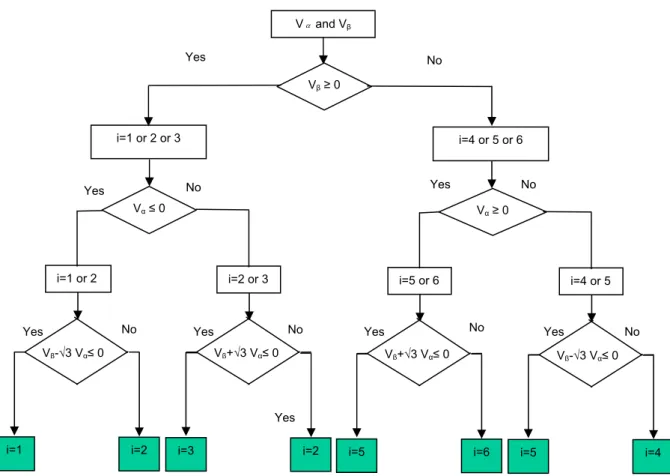
Figure 4-5. Sector Determination Algorithm.

In all cases, it is needed to determined sector number « i » where is located the vector Vi . To reduce time execution computing

δ

i et

δ

i+1, we have used this

algorithm.

In that way,

δ

i et

δ

i+1 are calculated directly from Vα and Vβ:

1 1 + +

⎥

⎦

⎤

⎢

⎣

⎡

+

⎥

⎦

⎤

⎢

⎣

⎡

=

⎥

⎦

⎤

⎢

⎣

⎡

i i i i

V

V

V

V

V

V

β α β α β α

δ

δ

And so

⎭

⎬

⎫

⎩

⎨

⎧

⎥

⎦

⎤

⎢

⎣

⎡

Π

+

⎥

⎦

⎤

⎢

⎣

⎡

⎟

⎠

⎞

⎜

⎝

⎛

−

=

⎥

⎦

⎤

⎢

⎣

⎡

+

0

1

)

3

(

0

1

)

1

(

3

3

2

1

p

i

i

p

E

V

V

i i

π

δ

δ

β α Vαand Vβ Vβ≥ 0 i=1 or 2 or 3 Vα≤ 0 i=1 or 2 Yes Yes Yes i=1 i=2 No i=2 or 3 i=3 i=2 No n No i=4 or 5 or 6 Vα≥ 0 i=5 or 6 Yes i=5 i=6 No i=4 or 5 i=5 i=4 No No No Vβ-√3 Vα≤ 0 Vβ+√3 Vα≤ 0 Vβ+√3 Vα≤ 0 Vβ-√3 Vα≤ 0

Yes Yes Yes

AVR32723

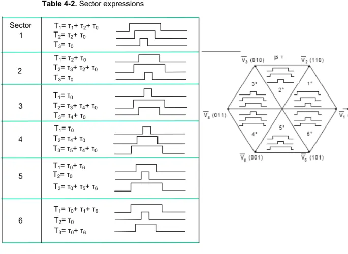
Table 4-2. Sector expressions

1 T1= τ1+ τ2+ τ0 T2= τ2+ τ0 T3= τ0 T1= τ2+ τ0 T2= τ3+ τ2+ τ0 T3= τ0 T1= τ0 T2= τ3+ τ4+ τ0 T3= τ4+ τ0 T1= τ0 T2= τ4+ τ0 T3= τ5+ τ4+ τ0 T1= τ0+ τ6 T2= τ0 T3= τ0+ τ5+ τ6 T1= τ0+ τ1+ τ6 T2= τ0 T3= τ0+ τ6 2 3 4 5 6 Sector

AVR32723

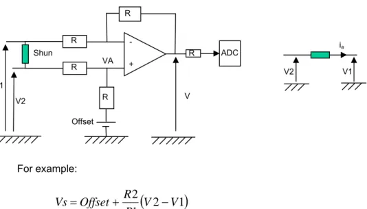
4.3 Current Measurement Stage

Three identical shunts are used to read the current Ia,Ib and Ic. These values should be amplified to be in the range of the ADC. Indeed, if we measure current of several milliamps (500mA), the maximum voltage is around 0.025V.

Figure 4-6. Amplifier stage

For example:

(

2

1

)

1

2

V

V

R

R

Offset

Vs

=

+

−

When measuring the three currents Ia,Ib and Ic, only two measures are required, indeed Ia + Ib + Ic = 0.

Figure 4-7. ADC and PWM synchronization

The ADC measures are done every period of the PWM. The first ADC measure should be done in the time range named tm. This time is the minimum time where

none of the 3-phases are driven. For example:

In case of sector 1, T1 is the longest time so it means that T1 > T-tm, in that case it is not possible to measure Ia. So Ib and Ic are measured and Ia is derived from the two others measures with the equation Ia = –Ib –Ic.

T T PWM tm tm tm ADC _t T1 R R R R - + R ADC V VA Shun V2 V1 Offset ia V2 V1

AVR32723

4.4 Current regulation and speed Regulation

4

In order to reduce time consuming effect of regulator, we have used the Integrator Proportional (IP) regulator.

4.4.1 Current Regulation

In a continuous domain, the closed loop has the mathematical expression: dref i d c i d

I

K

s

K

R

s

L

K

I

+

+

+

=

)

(

2

It is possible to easily identify the second order of the transfer function:

2 2

2

n

s

n

s

a

ω

ω

ε

+

+

With

K

i

=

L

c

ω

_n

and

K

d

=

2

εω

_n

L

c

−

R

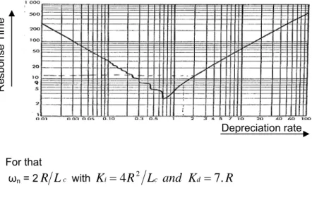
2

These correctors have been chosen to have a depreciation rate ε =2 and a response time of 5℅ (TrWn).

Figure 4-8. Response time vs Depreciation rate.

For that

ωn = 2

R

L

c with

K

i

=

4

R

2

L

c

and

K

d

=

7

.

R

4.4.2 Speed Regulation

The external closed loop for speed regulation has the following mathematical expression: 2 2 2

2

n n iv dv i ref

s

s

a

K

s

K

s

J

K

ω

ω

ε

+

+

=

+

+

=

Ω

Ω

With

J

K

et

J

K

dv n iv n

=

ε

ω

=

ω

2

2

4 _{The PI regulator is implemented as a software library component in the software} package associated with this application note. See also section 5.

Depreciation rate Re sp on se T ime

AVR32723

We choose ωn=0.1R/Lc and ε=2, So

J

L

R

K

et

J

L

R

K

c dv c iv

0

.

01

0

.

4

2 2

=

=

4.5 Execution Time and Regulation Loop

The following table gives the number of operations for each function

Table 4-2. Operations costs

Function Add Mul Div Shift

Concordia abc-to- αβ 7 0 0 17 Clark αβ-to-dq 2 4 0 62 Clark Inv dq-to- αβ 2 4 0 62 Regulation 7 4 0 124 Decoupling5 3 5 0 62 SVPWM 27 0 0 354

5 _{The decoupling stage is the stage to separate torque and power loss regulations} after the current measurement stage. The idea is to be sure to only regulate torque (without disturbing the power loss loop).

AVR32723

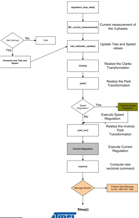
4.6 General Algorithm

As shown in Figure 4-9, the regulation_loop_task() process is sequenced on tick

reference (every 100µs). This task synchronizes current measurement and computes all mathematical transformations to execute the Field Oriented Control algorithm. Inside this task, there are two regulation loops interlinked:

- Current regulation loop. - Speed regulation loop.

Figure 4-9.Regulation Loop Task Step Machine

MC_current_measurement()

park_inv()

Speed Regulation?

Yes Proceed Speed Regulation No Execute Speed Regulation Compute new vectorial command regulation_loop_task()

Hall Interrupt No Wait

Yes

hall_estimator_update()

park() Clarke()

svpwm()

Message Ready? Prepare New Message for the HMI CDC Task

Compute new Teta and Speed

Sleep()

Current measurement of the 3-phases Update Teta and Speed

values

²

Realize the Clarke Transformation Realize the Park

Transformation

Realize the Inverse Park Transformation Current Regulation Execute Current

AVR32723

5 Source Code Architecture

5.1 Software Architecture

Figure 4-10.Software Architecture

This application does not require any operating system to run. The main() function is in charge of calling the software «tasks» (using a scheduler) realizing FOC algorithm computation and USB communication with the Communication Device Class (CDC) for HMI management. There are 2 tasks:

• regulation_loop_task()The regulation task that computes all calculation for

dedicated FOC algorithm.

• usb_task() / device_cdc_task()The USB Task: This task is in charge of the

CDC communication management.

The main loop of the application is a simple free-running task scheduler:

while(TRUE) { #ifdef USB_DEBUG usb_task(); device_cdc_task(); #endif mc_regulation_task(); } Motor Driver mc_driver.c

Field Oriented Control application

main.c

DRIVERS

usb.c adc.c pwm.c flashc.c pm.c gpio.c

Motor Control mc_control.c CDC communication task HMI device_cdc_task.c

Motor Control Library

PARK

SERVICES/MOTOR/PARK

Space Vector Modulation

SERVICES/MOTOR/SVPWM CLARKE SERVICES/MOTOR/CLARKE HALL ESTIMATOR SERVICES/MOTOR/HALL PI Regulator SERVICES/MOTOR//PI usb_task() device_cdc_task() regulation_loop_task()

AVR32723

5.2 Package

The EVK1101-SENSOR-FIELD-ORIENTED-CONTROL-X.Y.Z.zip contains projects for AT32UC3B0256 RevF or later:

• EVK1101-SENSOR-FIELD-ORIENTED-CONTROL-X.Y.Z

Default hardware configuration of the project is to run on the EVK1101 board, although any board can be used (refer to section 5.5.5)

5.3 Documentation

For full source code documentation, please refer to the auto-generated Doxygen source code documentation found in:

• AVR32723/APPLICATIONS/EVK110x-MOTOR-CONTROL/BLDC-FOC/EXAMPLE/readme.html

5.4 Projects/ Compiler

The IAR™ project is located here:

• src/ APPLICATIONS/EVK110x-MOTOR-CONTROL/BLDC-FOC/EXAMPLE/IAR/

The GCC makefile is located here:

• src/ APPLICATIONS/EVK110x-MOTOR-CONTROL/BLDC-FOC/EXAMPLE/GCC/

The Avr32Studio project is located in the root-dir of the package: -./

5.5 Implementations Details

5.5.1 Main()

The main() function of the program is located in the file:

• src/APPLICATIONS/EVK110x-MOTOR-CONTROL/BLDC-FOC/EXAMPLE/main.c

This function will:

• Initialize PWM outputs for Space Vector Generation.

• Initialize ADC inputs for 3-phases current measurement.

• Initialize USB connection for CDC HMI connection.

5.5.2 Motor Control Library

The motor control library is located here: • src/SERVICES/MOTOR_CONTROL/

This folder delivers:

• The Park and Clarke transformations explained in section 4.1.1 are delivered in the folder src/SERVICES/MOTOR_CONTROL/PARK_CLARKE/

• The Space Vector Modulation explained in section 4.2.1 is delivered in the folder

AVR32723

5.5.3 HMI CDC Task

The HMI CDC Task is located here:

• src/APPLICATIONS/EVK110x-MOTOR-CONTROL/BLDC-FOC/EXAMPLE/device_cdc_task.c

This task receives and sends messages through the USB communication. With:

• The message definition located in src/APPLICATIONS/EVK110x-MOTOR-CONTROL/BLDC-FOC/EXAMPLE/ENUM/frame.h

5.5.4 AT32UC3B Drivers

The example firmware uses the AVR32 UC3 driver library available in • src/UTILS/LIBS/DRIVERS/AT32UC3B/

5.5.5 Board File Definition

The application is designed to run on the EVK1101. All projects are configured with the following

define: BOARD=EVK1101. The EVK1101 definition can be found in the src/BOARDS/EVK1101 directory.

5.5.5.1 Board customization

For IAR project, open the project options (Project -> Options), choose the «C/C++ Compiler», then «Preprocessor». Modify the BOARD=EVK1101 definition by BOARD=USER_BOARD. For GCC, just modify in the config.mk file (src/APPLICATIONS/EVK110x-MOTOR-CONTROL/BLDC-FOC/EXAMPLE/GCC) the DEFS

definition with –D BOARD=USER_BOARD. For Avr32Studio, open the project properties (Project -> Properties), go in the «C/C++ build», then «Settings», «tool settings» and «Symbols». Modify the BOARD=EVK1101 definition by BOARD=USER_BOARD.

5.6 Project Configuration

The project configuration files can be found in the src/APPLICATIONS/EVK110x-MOTOR-CONTROL/BLDC-FOC/EXAMPLE/CONF/ directory.

Configuration files are not linked to IAR, GCC or Avr32Studio projects. The user can alter any of them, then rebuild the entire project in order to reflect the new configuration.

ƒ /CONF: configuration header files of demo modules:

CPU settings , Peripheral Clock settings and Motor settings

5.7 GUI Application

The GUI application installer is located here:

• src/APPLICATIONS/EVK110x-MOTOR-CONTROL/BLDC-FOC/LABVIEW/FOC_Gui.msi

The USB driver is located here:

AVR32723

5.8 CPU Cost and Memory Usage for Sensor Field Oriented Control algorithm.

All results are given using IAR Workbench 5.3 compiler revision 3.10A with speed optimization level and Hmatrix optimization.

Criteria Result

CPU Occupation 35% with a tick

value of 100 us at 42MHz.

Code Size 17Kb

Data 13Kb

Const 3.5Kb

5.9 Limitation of the Sensor Field Oriented Control algorithm.

All the application has been implemented with a fixed point library written in a 32-bit format (Q1.31)6.

The usage of this library allows accelerated computations but it generates some limitations in the variation range of each variable.

For example, when computing current regulation, every ADC samples are scaled by a variable named E. This variable matches a ratio of the bus voltage. In the current implementation, this variable has been fixed to half of the nominal voltage of the motor. In that case, the nominal speed is equal to 2000 rpm.

6 _{See the application note:}

AVR32723

5.10 Compiling the application

The following steps show you how to build the embedded firmware according to your environment.

5.10.1 If you are using AVR32Studio

• Launch avr32Studio

• Create a new AVR32 C project («File» -> «new» -> «AVR32 C Project»).

• Fill-in the dialogue box with project name, set target MCU to UC3B0256 and press finish.

• Choose Import archive file («File» -> «import»…), press the “next” button.

• Select the EVK1101-SENSOR-FIELD-ORIENTED-CONTROL-X.Y.Z.zip archive file with the browse button. Select «into folder», check «Overwrite existing resources without warning» and press the “finish” button.

• The project is now available in the given project name.

• Press the build button

• Load the Code: Please refer to the application note AVR32723: AVR32 Studio getting started

5.10.2 If you are using GCC with the AVR32 GNU Toolchain

• Open a shell, go to the src/APPLICATIONS/EVK110x-MOTOR-CONTROL/BLDC-FOC/EXAMPLE/GCC/ directory and type:

make rebuild program run

5.10.3 If you are using IAR Embedded Workbench® for Atmel AVR32

• Open IAR and load the associated IAR project of this application (located in the directory

src/APPLICATIONS/EVK110x-MOTOR-CONTROL/BLDC-FOC/EXAMPLE/IAR)

• Press the “Debug” button at the top right of the IAR interface.

• The project should compile. Then the generated binary file is downloaded to the microcontroller to finally switch to the debug mode.

AVR32723

5.11 Start the PC application

• Plug the EVK1101 to the PC through a USB Connection.

• The USB enumeration should start; a new serial port appeared in Windows.

• Power-up the power bridge.

5.11.1 Field Oriented Control GUI

Once the GUI is launched, the user can select a serial port number and connect the application.

Figure 4-11. Field Oriented Control GUI

5.11.1.1 Increase Speed Value

When the speed reference increases with constant resistive torque value, the Iq increases smoothly to target the new speed value. The Id remains at ‘0’.

Figure 4-12. Increase Speed Value Step

When the user want to increase speed value

Speed Iq Iq Id Speed Serial port

AVR32723

5.11.1.2 Increase Resistive Torque Value

The resistive torque value increases so the measured speed value decreases. To compensate it, the FOC algorithm should increase the Iq reference and finally the speed is regulated. The Id remains at ‘0’.

Figure 4-13. Increase Resistive Torque Value Step

Speed

AVR32723

6 Reference

[1] Commande vectorielle sans capteur de position d'une machine synchrone à aimants permanents – Atmel Nantes & IREENA-

AVR32723

7 Appendix

Disclaimer Headquarters International Atmel Corporation 2325 Orchard Parkway San Jose, CA 95131 USA Tel: 1(408) 441-0311 Fax: 1(408) 487-2600 Atmel Asia Unit 1-5 & 16, 19/F

BEA Tower, Millennium City 5 418 Kwun Tong Road Kwun Tong, Kowloon Hong Kong Tel: (852) 2245-6100 Fax: (852) 2722-1369 Product Contact Atmel Europe Le Krebs

8, Rue Jean-Pierre Timbaud BP 309 78054 Saint-Quentin-en-Yvelines Cedex France Tel: (33) 1-30-60-70-00 Fax: (33) 1-30-60-71-11 Atmel Japan 9F, Tonetsu Shinkawa Bldg. 1-24-8 Shinkawa Chuo-ku, Tokyo 104-0033 Japan Tel: (81) 3-3523-3551 Fax: (81) 3-3523-7581 Web Site www.atmel.com Technical Support [email protected] Sales Contact www.atmel.com/contacts Literature Request www.atmel.com/literature

Disclaimer: The information in this document is provided in connection with Atmel products. No license, express or implied, by estoppel or otherwise, to any

intellectual property right is granted by this document or in connection with the sale of Atmel products. EXCEPT AS SET FORTH IN ATMEL’S TERMS AND

CONDITIONS OF SALE LOCATED ON ATMEL’S WEB SITE, ATMEL ASSUMES NO LIABILITY WHATSOEVER AND DISCLAIMS ANY EXPRESS, IMPLIED OR STATUTORY WARRANTY RELATING TO ITS PRODUCTS INCLUDING, BUT NOT LIMITED TO, THE IMPLIED WARRANTY OF MERCHANTABILITY, FITNESS FOR A PARTICULAR PURPOSE, OR NON-INFRINGEMENT. IN NO EVENT SHALL ATMEL BE LIABLE FOR ANY DIRECT, INDIRECT, CONSEQUENTIAL, PUNITIVE, SPECIAL OR INCIDENTAL DAMAGES (INCLUDING, WITHOUT LIMITATION, DAMAGES FOR LOSS OF PROFITS, BUSINESS INTERRUPTION, OR LOSS OF INFORMATION) ARISING OUT OF THE USE OR INABILITY TO USE THIS DOCUMENT, EVEN IF ATMEL HAS BEEN ADVISED OF THE POSSIBILITY OF SUCH DAMAGES. Atmel makes no representations or warranties with respect to the accuracy or completeness of the

contents of this document and reserves the right to make changes to specifications and product descriptions at any time without notice. Atmel does not make any commitment to update the information contained herein. Unless specifically provided otherwise, Atmel products are not suitable for, and shall not be used in, automotive applications. Atmel’s products are not intended, authorized, or warranted for use as components in applications intended to support or sustain life.

© 2009 Atmel Corporation. All rights reserved. Atmel®_{, Atmel logo and combinations thereof, AVR}®_{, AVR Studio® and others, are the} registered trademarks or trademarks of Atmel Corporation or its subsidiaries. Windows® and others are registered trademarks or trademarks of Microsoft Corporation in the U.S. and or other countries. Other terms and product names may be trademarks of others.