Macroeconomic Input-Output modelling –
structures, functional forms and closure rules
Kurt KRATENA* & Gerhard STREICHER
Austrian Institute of Economic Research (WIFO), Joanneum Research (JR)
ABSTRACT: This paper gives an outline of options and strategies for closing input-output (IO) models by stepwise endogenisation of variables and embedding the input-output core into a general macroeconomic model. The accounting framework is a modified linear static IO model built around Supply and Use tables as provided by EUROSTAT. The modifications take into account that some variables that are determined in the IO quantity and price model will be taken from econometric modelling blocks for production, trade and the price system. The process of endogenising and modelling comprises the different steps of (i) endogenising final demand and factor demand (ii) applying macroeconomic closure rules and (iii) full modelling of factor markets. Step (i) comprises the endogenisation of totals of demand as in macroeconomic models or in SAM multiplier models as well as the linking of quantities and prices. Different types of IO models (type I to IV), econometric IO models (EIO) and computable general equilibrium models (CGE) can then be identified as different combinations of these modelling steps. Viewed in this way, the often almost “tribal” controversies between the CGE community and the econometric modellers look somewhat exaggerated.
KEYWORDS: Input-output models, CGE models
2 1. Introduction
Research on extending the static input-output (IO) model to a dynamic or full macroeconomic model looks back to a history of about 50 years. One path of further developing the static IO model is represented by the dynamic IO model, first formulated by Leontief himself, where investment expenditure is integrated in the IO framework and thereby endogenized.
The development of the first fully formulated macroeconomic IO model is closely linked to the name of Richard Stone, who in parallel worked on the extension and further development of national accounts in the direction of social accounts in a matrix representation (the 'SAM'). From about 1960 on the first publications outlining a research strategy based on input-output modelling that later should be known as the 'Cambridge Growth Project' appeared (Stone and Croft-Murray, 1959, Stone, 1960 and Cambridge DAE, 1962). Another pioneer in extending the input-output core to a full multisectoral macroeconomic model was Johansen (1960). Two important features of these models were the endogenization of parts of final demand (usually exogenous in the static IO model) and the modelling of demand components depending on (relative) prices. The Johansen as well as the Stone model can be seen as important first steps of the CGE models developed later by Scarf, Shoven and Whalley (Scarf and Shoven, 1984; Shoven and Whalley, 1984).
Later on the research group working on the Cambridge Growth Project developed a fully fledged macroeconomic multisectoral model of the UK economy (Barker, 1976; Barker and Peterson (1987)). At the same time another model project started in the US with the
development of a macroeconomic closed IO model known as INFORUM (Inter-industry Forecasting and Modelling at the University of Maryland) first described in Almon et.al. (1974). The INFORUM project expanded to the scope of an international model by linking
3 similar national models via bilateral trade matrices (Almon, 1991 and Nyhus, 1991). Both the UK model MDM as well as the INFORUM models incorporate econometric specifications that take into account economic theory but cannot be directly derived from utility
maximization or cost minimization behaviour. The models are dynamic due to the
econometric specification, but not dynamic in the sense of dynamic optimization with a given rule of expectation formation.
The development of large CGE models based on an IO core model mostly took place in parallel during the 1970es and the 1980es and arrived at models directly linked to the SAM structure of national accounts. For international trade the CGE models apply the Armington assumption that the same commodity from different origins represents different commodities that are non-perfect substitutes with substitution elasticities from a CES function (Armington, 1969; Reinert and Roland-Holst, 1992). In the literature on international one finds specific CGE models for the analysis of international trade (typical examples are Bergstrand and Baier, 2000; Baldwin and Robert-Nicoud, 2007) that also include different specifications of trade, especially the differentiation between trade in final and intermediate goods, which is available in the IO data base. In the standard applied CGE model (Lofgren, et.al., 2002; Hertel and Tsigas, 1997) this differentiation between final and intermediate goods trade is usually incorporated in the database (like in GTAP), but has no explicit correspondence in modelling. Instead the CES function approach based on Armington (1969) is applied to both types of international trade. From about 1990 on issues of environmental policy pushed the
development of CGE models like the GREEN model of OECD (Burniaux, et.al., 1992; Lee, et.al., 1994). The situation in Europe during the decade after 1990 was characterized by the parallel development and application of the CGE model GEM-E3 (Conrad and Schmidt,
4 1998) and the EIO model E3ME (Barker, 1999, Barker, et.al., 1999). Both models integrated energy and emissions in the economic model (E3) and have been used for evaluation of energy tax policies and emission trading at the EU level in standardized simulations (for comparison of results see: Barker, 1999).
Different types of EIO models have been developed since 1990 for the regional level, especially by the team of Geoffrey Hewings (REAL, Univ. of Illinois) based on the Washington Projection and Simulation Model (Conway et al, 1990). Another important example of a recently developed EIO model is the global (fully interlinked) model that has been developed by the team of Bernd Meyer and his team (GWS), starting from a prototype model COMPASS (Uno, 2002, Meyer,Uno, 1999) and leading to the GINFORS model (Lutz, et.al., 2005 and www.mosus.net).
As a consequence of these parallel developments of very different models, there has been an ongoing discussion between the EIO- and the CGE-community focussing on the following issues: calibration vs. econometric estimation, the choice of functional forms in relation to the behavioural assumptions (economic rationality of agents), the role of equilibrium mechanisms and of the – mostly arbitrarily chosen – benchmark year. In this debate Jorgenson (1984) stressed the importance of econometric methodology in order to derive the parameters of CGE models, whereas Shoven and Whalley (1984) characterized econometrics as unviable for this purpose partly due to the data requirements and to the fact that actual timer series also contain non-equilibrium states of the economy. Actually calibration as the methodology for deriving parameters is very much linked to the concept of equilibrium in CGE models. McKitric (1998) engaged in the discussion about functional forms and could demonstrate that the choice of the functional form together with the choice of the benchmark year has a substantial
5 influence on the results of policy evaluation. The conflicting positions between the EIO- and the CGE-community can be described by different underlying assumptions about rationality of economic behaviour. The utility maximization and cost minimization approach of CGE models conflicts with the concept of 'bounded rationality' (Lutz, et.al., 2005) of EIO models, the respective critique is characterized by terms like 'theory with numbers' and 'ad hoc specification without theory'. An interesting and exhaustive overview of this debate can be found in Grassini (2004).
Despite this ongoing debate and the sometimes almost „tribal‟ controversies between EIO and CGE modelling, there are almost no studies that attempt a systematic overview and analysis of pro‟s and con‟s of different approaches. The approach of Jorgenson and the study by McKitrick (1998) attempt to reconcile the different methodologies of CGE and EIO models, especially econometric techniques and calibration. An important study that deals with a systematic account and comparison of the different modelling approaches is West (1995), which relates to the level of regional modelling. West (1995) also concludes that some convergence between the different approaches might occur and is desirable.
In this paper we synthesize the different approaches of macroeconomic model building around an IO core in a systematic way and describe the main features of a full model and the single steps to arrive at it. This systematic approach allows us to bridge some gaps between EIO models and CGE models and thereby isolate clearly the essential differences between the two modelling approaches. We propose a research strategy orientated along the lines of easily accessible international data bases and incorporating recent developments in economic theory, especially in the field of consumer and production theory as well as international trade.
6 2. The SUT accounting framework: a static quantity and price model
In the following the accounting framework of a macroeconomic IO model shall be lined out, based on data of supply and use tables (SUT), which have become the standard presentation of IO statistics at EUROSTAT and also at many other statistical offices around the world. The building blocks in terms of datasets for this accounting framework are:
- The Supply matrix V (commodities * industries), containing domestic output at basic prices (commodities) plus imports (c.i.f.) plus trade and transport margins plus taxes net subsidies. The row sum of this matrix therefore gives the total supply at purchaser prices by
commodities
- The Use matrix Upp (commodities * industries) of total use at purchaser prices
- The Use matrix T of trade and transport margins and of taxes net subsidies (by summing up these 3 matrices)
- The Use matrix Umbp (commodities * industries) of total imported use at basic prices
These building blocks define some maximum that could be directly available in IO statistics for several base years or even a short time series (as is the case for EU 15). In some cases the information on matrix T and matrix Umbp is restricted and had to be estimated. The building
blocks for this estimation were then taken from the more complete information of symmetric (homogenous branches) IO tables in base years.
Given these building blocks the first step was taking into account the general difference how margins and taxes/subsidies affect the difference between use in basic and in purchaser prices. Accounting for margins does not change the column sum of the use matrix, as it just shifts values from entries in manufacturing rows to the rows of the margin producers (trade and
7 transport). This is not the case for taxes and subsidies, which change the total input value of intermediates in an industry. Therefore the set of goods is expanded by a „dummy‟-good called “taxes net subsidies”. The advantage of this formulation is that taxes and subsidies do not leave the system and total use in purchaser prices and basic prices is the same for each industry (column) of both use matrices.
Building up the model then starts with calculating the product mix matrix (column sum = 1) C from the supply matrix and the market shares matrix D (column sum = 1) from the make matrix (= the transposed supply matrix):
1
ˆ
V
q
bpC
(1) 1 ˆ Vgbp D (2)In (1) and (2) the column vectors of output by industries in basic prices qbp and by
commodities in basic prices gbp have been transformed into diagonal matrices. In the quantity
IO model commodity technology will be applied making use of the product mix matrix C, whereas in the price IO model the market shares matrix D must be used.
The quantity model
The model structure is oriented along the lines of the description of the Stone model in Pyatt (1994) as well as the make-use model in a large EIO model in the UK model MDM (Barker, Peterson, 1987). The IO structures are only used to determine the commodity structure of given totals of intermediate and final demand (domestic as well as imported). This accounting framework allows for modelling total intermediate demand (domestic as well as imported) by factor demand functions in the production block and modelling final demand totals (domestic as well as imported) as well as their commodity structure in the block of final demand.
8 Starting point are therefore the use structure matrices calculated from both use matrices in purchaser prices. Note that due to including taxes net subsidies into the set of commodities, the column sum of all uses is always identical in basic and in purchaser prices. The matrix of the structure of total use in purchaser prices, Spp, is given by elements xij/si, where xij is the
single flow in the use matrix and si is the column sum of this matrix, i.e.:
1
ˆ Us
Spp (3)
The same is done for imported intermediates separately which allows for having imported inputs also determined in factor demand functions in the production block:
1 ˆ m m m bp U s S (4)Note that for imports this is done at the valuation of c.i.f., which corresponds to basic prices. We further use the adjusted import shares matrix (as described above) M with elements mij/xij,
where mij are the flows in the import use matrix (adjusted for the SUT base year) and xij are
defined as above.
We use the relationship between the elements of matrix Spp and of matrix Smpp together with
the column totals s and sm of both matrices to define the elements of the import shares matrix M:
mij/xij = (mij/smi) (smi/si) (si/xij) (5)
The quantity model can then be written in the following form:
s S Upp pp (6) T U Ubp pp (7)
9 pp pp d bp U MU U (8) i F i U gbpd bpd bpd (9) bp d bp q g C1 (10)
The model is solved by iteration for the equilibrium value of qbp. In (6) describes an
element by element multiplication procedure. This structure is set up for the interaction with a production block, where total demand for intermediates s by industry is determined for a given output vector qbp which comes from equation (10).
The matrix of domestic final demand
F
bpd in (9) is derived from a matrix of total final demandpp
F
in purchaser prices applying the same margin matrix as in (7) and the same import shares matrix as in (8). The matrix of final demand comprises the column vectors of privateconsumption, gross fixed capital formation, public consumption and exports:
pp pp pp pp
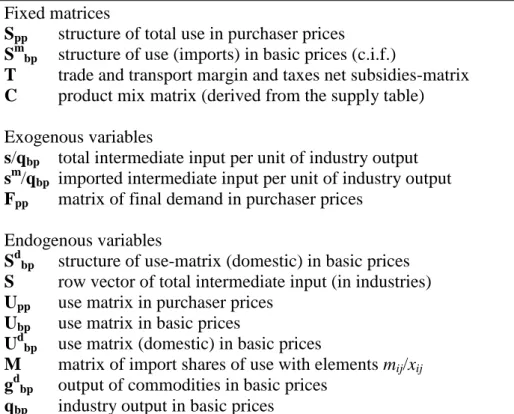
pp cp in cg ex F , , , (11) T F Fbp pp (12) bp bp d bp F MF F (13)The model structure therefore can be defined as in Table 1 in terms of given and fixed matrices, exogenous and endogenous variables. The exogenous variables partly are determined in the econometric models built around the IO core.
10 The price model
The general assumption of the linear static model is the law of one price (Pyatt, 1994), i.e. each domestic and imported commodity price is identical for all users. This model can be seen as a model of „minimum price differentiation‟, which often is not supported by data in cases of availability of IO tables at constant prices. Some statistical offices deal with a model of „maximum price differentiation‟ in the process of deflating IO tables, where each user in the same row of the use matrix faces a different price. This procedure is correct from a statistical point of view, as the usual level of aggregation in SUT does not guarantee that different cells in the same row of the use matrix contain the same bundle of (sub-) commodities.
In CGE models a model of price differentiation is usually applied taking into account the differentiation between domestic flows of goods and goods in international trade as contained in the GTAP-database. Therefore each commodity dependent on the destination of the
corresponding flow is valued at five different prices (s.: Lofgren, et.al., 2002):
the domestic commodity price, pd, the export price, pex , the import price, pm, the domestic price for domestic users, pdd, and the composite goods price, pg.
One composite price in this model therefore is this composite goods price pg for each user and each good, defined as the weighted average of the good‟s domestic price and the import price, the weight being the import share mij/xij. The other composite price is the domestic
commodity price, pd, which is the weighted average of the export price and the domestic price for domestic users, pdd. As only the domestic commodity price and the export price can be observed from statistics, the price must be calculated from the data. The two composite prices are given by commodity balances for imported, exported and domestic deliveries:
11 d i i ex i dd i dd i d i x ex p x p p (14) i i m i dd i dd i g i x m p x p p (15)
In (14) the xd , xdd, m and ex are the corresponding quantity flows to the prices that are differentiated in the price system. In analogy to the quantity model only the structure of the use matrix is used in the price model, which again corresponds to a model where the vector of total intermediate input s might be determined from factor demand functions. In a first step therefore the row vector of prices of intermediate inputs in each industry is determined by using the two use structure matrices for domestic goods and imports (Sdpp and Smpp). In this
equation therefore price differentiation between domestic commodities for domestic use and imported commodities is taken into account and the matrices of margin and tax rates, Tt are used. The price vector for total intermediate inputs ps can be treated as in (16) or separately for the two components of domestic and imported intermediate costs. Assuming that the IO model is linked to a model of the production side, where the total intermediate input s is determined, the price ps or its components will enter as independent variables in this production block. It might make sense to model pricing behaviour simultaneously in this production block depending on the market form in the goods markets. In that case the output prices by industry, pq would be determined by average or marginal costs, including the costs
of domestic and imported intermediates, ps s/qbp as well as labour costs, w l/qbp with labour
input l and the wage rate w. If the input coefficients s/qbp and l/qbp as well as the output price
12 calculated as a residual. Finally this output price is converted into a domestic commodity price pd by using the market shares matrix and thereby assuming industry technology.
m bp t m d bp t dd S p T S p T S p (16) r = pq - ps s/qbp - w l/qbp (17) D p pd q (18)
Inverting equation (14) can then be used to derive the domestic price for domestic use and the model can be solved for given import and export prices and output prices that are determined together with factor inputs in a separate production block. Additionally the use structure and market shares matrices must be given.
dd i i ex i d i d i dd i x ex p x p p (19) TABLE 2
A general approach of dealing with deflation and different levels of pricing (basic and
purchaser prices) is to measure all variables in the quantity model always in current prices and purchaser prices and to apply the deflation procedure to arrive at variables at constant prices and basic prices. In this step the margins (both at current and at constant prices) are also determined.
The accounting framework is finally closed from the macroeconomic side by adding the definitions for GDP, household disposable income and total national saving. GDP at factor costs is directly given by total value added, calculated by multiplying the row vector of value
13 added-coefficients with the column vector of output at basic prices. Subtracting from GDP the part of gross operating surplus not accruing to households and adding all flows between households, government and ROW (direct taxes, THH, social security contributions, TsHH, and social and other transfers, TrHH) yields disposable income of households, YD.
Total national savings S comprises households' savings SHH (the difference between income
YD and consumption pCCP) and foreign savings Sf (the negative of the current account
balance). Ex post savings must equal total investment I, how this equilibrium is reached depends on the macroeconomic closure rule.
GDP = (w l/qbp + r)*qbp (20)
YD = GDP – R - THH - TsHH + TrHH (21)
SHH = YD – pCCP (22)
Sf =pmM – pexEX (23)
S = SHH + Sf ≡ I (24)
The model outlined here solves as the traditional static IO model and deals with deflation and different price concepts in one step. Adding the macroeconomic equations (20) to (24) gives an accounting framework containing all information normally also contained in a SAM. By simply linking value added and final demand we would end up with a simple SAM multiplier model equivalent to what West (1995) has labelled a simplified IOE model.
14 In the static IO model framework lined out above the vectors of the final demand components (both domestic as well as imported commodities) were assumed to be exogenous in nominal terms. Concerning final demand components in most models public consumption is treated as a policy variable and therefore exogenous and exports are directly determined by completely exogenous variables, either in a stand-alone national model by foreign demand or in a multi-regional model by imports of trading partners. In CGE models the export supply additionally depends on the relative price of exports (pex) and domestic commodities for domestic use (pdd).
One important component making up a large part of final demand that in a fully formulated EIO model should be modelled is private consumption. It must be noted that endogenizing private consumption in a multisectoral model always has a twofold perspective, namely determining the total (the column sum) of consumption as well as the commodity structure. The procedure of endogenising consumption therefore comprises the two steps of (i)
including the total demand component and linking it to other macroeconomic aggregates as in the SAM multiplier model and (ii) the linking of quantities and prices in a fully formulated demand model.
Endogenising aggregate consumption
In the SAM multiplier model as well as in CGE models the expenditure side of household accounts is linked to the income side by fixed shares. These fixed shares can be applied to the flows between households and government as well as to the savings or consumption
propensity. In CGE models the kind of combination of fixed shares with fully exogenous variables in the household accounts depends on the macroeconomic closure rule (see: Lofgren, et.al., 2002), so that macroeconomic equilibrium conditions in other accounts (for
15 example foreign savings) determine the consumption behaviour of households. This linking of equilibrium conditions to household consumption behaviour adds some dynamics to the relationship between household income and consumption expenditure that is absent in a pure SAM multiplier model.
The alternative of introducing dynamics in household consumption behaviour and equally applying macroeconomic equilibrium conditions in an EIO modelling framework is to
econometrically estimate an error correction model of private consumption. At the same time the fixed shares between household income and flows to government can also be modelled in dynamic behavioural equations by introducing short and long term elasticities of tax revenues to households' income. In (26) and (27) the general functions for direct taxes and social security contributions are described, where the first depend on gross household (primary) income and the latter only on gross wage income. A dynamic specification could be chosen along the lines of the 'Autoregressive Distributed Lag'-Model (ADL), from which short and long term elasticities of variables can be derived.
THH = THH ((w l/qbp + r)*qbp - R) (25)
TsHH = TsHH (w l/qbp *qbp ) (26)
The equilibrium concept for private consumption introduced in an EIO model can be based on the econometric concept of co-integration of variables as lined out in Engle and Granger (1991). Starting point is the the assumption of a long-run equilibrium relationship between households income and consumption expenditure, that can be statistically tested applying the theory of time series. In terms of measurement the issue of interplay between current income and changes in net wealth of households is of course essential in such a setting. If these
16 dynamic stock-flow interactions are correctly taken into account in the empirical
measurement of 'income' this simple equilibrium relationship-approach can be seen as equivalent to other dynamic models of consumption. Econometrically one starts by first estimating the long-run relationship between total private consumption of households, CP and deflated disposable income, YD/pC and testing for co-integration (t is a time index):
CPt 0 1log
YDt /pC,t
tlog (27)
If co-integration can be detected one can proceed by setting up the dynamic model, either in the format of the two steps in one-procedure of the error correction-model by Engle and Granger (1991) or as an ADL-model, which can be shown to be equivalent to the error correction model (Banerjee, Dolado, Galbraith, Hendry, 1993):
CPt
YDt pCt
CPt
YDt pCt
tlog 0 1 log / , 1 0 1log 1/ ,1 (28a)
CPt 0 1log
CPt1
0log
YDt /pC,t
1log
YDt1/pC,t1
tlog (28b)
From both specifications a short- and long-run elasticity of consumption can be derived and from (28a) also the speed of adjustment to equilibrium can be seen.
In general this model of household consumption and interaction between government and households is very similar to a CGE model: it incorporates an equilibrium mechanism and uses the detailed accounts for households and governments which are usually part of a SAM structure. Compared to a static CGE model the model outlined here runs explicit calendar-time and not in comparative static-mode, so that the adjustment to equilibrium is described as an explicit time path. In CGE models the dynamics and the adjustment to equilibrium mostly does not follow from the household consumption model itself, which is modeled by fixed
17 average propensities to consume, but from the interaction with the closure rules (see section 7).
Linking quantities and prices
The second step in modeling private consumption and thereby endogenising it in an EIO framework consists of describing the allocation of total household consumption CP among the commodities of the vector cppp in the SUT accounts. For this step a full integration of
prices and quantities is required, so that the commodity prices determined in the price system described in section 2 affect the allocation of the household budget. That leads to a full interaction between the price model and the vector of final demand in the quantity model of the SUT framework. In some models like GINFORS the allocation is modeled by single equations and directly applied to the vector cppp in the SUT accounts. This is also the case in
the standard CGE model (Lofgren, et.al., 2002).
In other EIO models the full data set of consumers' expenditure in National Accounts in the COICOP classification of consumption purposes is used, which must then be converted to the commodity classification CPA in the SUT framework. This is normally done by the
application of a bridge matrix which is in some cases officially available from Statistical Offices.
The allocation of total consumption across consumption purposes (in COICOP) can then be modeled in a demand system. The history of consumers' demand systems for EIO modeling starts with the linear expenditure system (LES) developed by Stone (1954), which is still standard in CGE modeling. One of the important advantages of LES is the property of regularity for the whole price-expenditure space, so that budget shares lie within the [0,1] interval. The disadvantage that in the end led to the development of more flexible functional
18 forms is the over-restrictive and inflexible property of mutual dependence of elasticities. It has been shown, that fixing a few price and income elasticities determines the whole elasticity set in LES.
The most important flexible functional form is the Almost Ideal Demand System (AIDS), developed by Deaton and Muellbauer (1980), which shows a high flexibility of substitutive and complementary relationships between commodities, according to the philosophy ‚let the data decide„. A well known disadvantage of the AIDS model is that additivity and regularity will not be granted for large income and price changes. That has led to suggestions of
modifying the underlying preference structure of the AIDS model in a way to arrive at a more stable model, like the additive model AIDSAD model (Rimmer and Powell, 1996) or the modified model MAIDS (Cooper, McLaren, 1992, 1996). A modification of the original AIDS model in order to allow for modeling empirically detected non-linear Engel curves was presented as the quadratic AIDS model, QUAIDS (Banks, Blundell, Lewbel, 1997). Another critique from the side of EIO modeling is that some microeconomic restrictions like Slutzky symmetry postulated in microeconomic theory for the 'representative consumer' need not to hold for market data as in National Accounts and are therefore 'over-restrictive. That has led Almon (1996) to present an alternative demand system PADS, the 'Perhaps Adequate Demand System'.
Starting point of the AIDS model is the expenditure function for private consumption CP(u, pi) with the arguments utility (u) and the vector of prices (for details of demand system
modelling in the EIO context, see: Kratena, Mongelli and Wueger, 2009): )) ( log( )) ( log( ) 1 ( ) , ( logC u pi u a pi u b pi (29)
19 with a Translog price index for a(pi) and a Cobb-Douglas price index for b(pi). As the level of
utility u is an argument of the expenditure function, an indirect utility function can be derived and by the application of Shephard's Lemma to the cost function the well known budget share equations for the i consumption purposes follow:
j i j ij i i P CP p w log log (30)In (30) the price index P can be approached by the Stone price index:
k k k p w P log log *
instead of using the original Translog price index of AIDS.
The budget shares wi (for i as the COICOP classification of consumption purposes) together
with the level of CP from equation (28) enable us to determine the vector of consumption in COICOP-classification and at purchaser prices, cpCC,pp. Using the above mentioned bridge
matrix (commodities,CPA * purposes, COICOP), BC, this vector can be transformed into the vector of private consumption, cppp:
cppp = BC cpCC,pp (31)
The transposed bridge matrix can on the other hand be used to link the price vector of goods prices, pg, to the price vector of COICOP consumption purposes:
pgCC = BC' pg (32)
The demand system together with these bridge matrix operations describes the full procedure of linking quantities and prices in the consumption block. The comparative advantage of the EIO approach presented here against the standard CGE model is a superior modeling of the explicit adjustment of total consumption to a long run macroeconomic equilibrium and a superior modeling of the budget allocation process by applying less restrictive functional
20 forms than LES. The critique of other EIO modelers like Almon (1996) about the
microeconomic 'over-restrictiveness' of models based on the representative consumer-concept can be overcome by explicitly capturing the impact of the aggregate household structure according to a list of characteristics on the budget allocation as in Kratena, Mongelli and Wueger (2009).
4. Modelling production: factor demand, investment and output prices
Concerning factor demand for intermediates the accounting framework lined out above assumes that only the totals of domestic and imported intermediates are determined and that the commodity structure is given by the fixed structure of the use matrices. CGE models (Lofgren,et.al. 2002 and Hertel and Tsigas, 1997) usually work with production or cost function approaches of the CES type in a nested structure of the production process. The factor demand for capital, labour, energy and other intermediate inputs (KLEM) is often modeled by combining CES and Leontief functions. Capital is usually a fully adjusting factor, as the comparative static CGE model deals with immediate adjustment to equilibrium
conditions. One shortcoming of the nested structure is the arbitrary introduction of
separability conditions, which might though be based on engineering expert judgment of the production process.
For the EIO approach outlined here we propose a flexible functional form (Translog or Generalized Leontief) of the dual cost function and factor demand framework (Berndt, 1991; Morrison, 1989, 1990). The dual cost function approach has been extended and further
developed during the last three decades by focusing on the following issues: (i) differentiating between fully variable inputs and short run fixed inputs (capital, part of the labor input), (ii)
21 incorporating different types of technical change (TFP, factor bias, emdodied and induced technical change), (iii) returns to scale, and (iv) imperfect competition in the goods markets. Capital as a short-run 'quasi' fixed factor has been used in several studies (Morrison, 1989 and 1990). In these models technical change is partly embodied in the capital stock and
investment is not directly determined from a factor demand function for capital. As capital is exogenous in the short run, a 'shadow price' of capital can be derived (Berndt and Hesse, 1986) that in a further step can enter an investment function. This can also be a link to price-induced technical change, as investment (capital stock adjustment) reacts to factor price changes (Kratena, 2007).
There are several ways of extending the dual cost function model with short-run fixed capital to a model incorporating investment demand. The simplest method consists of including an equation that explains adjustment of the short- run fixed capital stock to its long-run level. This can be done by a partial and ad hoc adjustment mechanism like a flexible accelerator mechanism. As Galeotti (1996) has pointed out, this mechanism describes a systematic ex post adjustment, where errors in the past are corrected but where expectations about the future development of exogenous variables play no role. In that sense this approach describes
backward looking behaviour and is only 'pseudo-dynamic'. Alternatives consist in explicitly taking into account internal adjustment costs of changing the capital stock like in Berndt, et.al. (1981) and in Watkins and Berndt (1992) or formulating a full dynamic model with
expectations formation mechanisms (Morrison, 1986 and Galeotti, 1996). The common functional form for most of these models is defined by a stock adjustment equation of the type:
22 where k is he actual stock and k* the optimal stock given by the condition that the 'shadow price' of capital equals the user costs, possibly complemented by other long-run conditions in the case of infrastructure investment (long term growth of output, population, labor force). From equation (33) an investment function in per industry follows that can be converted into the vector of gross capital formation inpp in final demand (11) by the matrix of capital
formation BI linking the investment by industries (and assets) to the investment commodity structure:
inpp = BI in (34)
The stock adjustment function can be embedded in a set-up of a cost function G in each industry comprising short-run variable costs VC
pv,k,Y,t
as well as expenditure for(aggregate) investment I with the corresponding price index of (aggregate) investment goods pI :
p k q t
p I VCG v, , , I (35)
where pv is a vector of variable input prices for input quantities v, k is the level of the
quasi-fixed input to production, q is the level of output (in our case given by the vector qbp) and t is
time. Taking into account that gross investment in this stock comprises changes in the stock plus depreciation with depreciation rate , we have:
p ,k,q,t
p (k k) VCG v I (36)
The producers choose a time path of k to minimize discounted costs over a time horizon for which values for the exogenous variables are given:
VC p k q t p k k
dt e rt t( v, , , ) I( ) min ( )
(37)23 where k stands for the change in k.
The two main optimality conditions following from this cost minimization problem are given by Shephard's Lemma and the envelope condition for the capital stock:
v p VC v I p r k VC ) ( .
The envelope condition in this simple case just states, that the shadow price of fixed assets (given by the negative of the term that measures the impact of capital inputs on short- run variable costs) must be equal to the user costs of capital. If this envelope condition is not fulfilled, the capital stock adjusts according to (33).
Shephard's Lemma gives the factor demand functions, in the case of the Translog function as cost shares in VC and in the case of the Generalized Leontief function as input coefficients in output. We propose to extend the KLEM-set of input factors by differentiating between imported and domestic intermediates, defined as the industry vectors sm and sd. Further splitting up total intermediate inputs into energy e and defining as sm and sd only the non-energy inputs, gives the following set of factor demand functions in the case of the Translog function (with i = l ,e, sm, sd):
p q k
VC i, bp, ;
p q k
VC e bp i, , ;
p q k
VC s bp i m , , ;
p q k
VC s bp i d , , (38)The vector of input prices pi is partly determined in the IO price model and comprises
d bp t dd S T p and m bp t m S T
p . The wage rate might be determined in a model of the labor market (section 6) and the energy price might be exogenous. An empirical application of this model is lined out in Neuwahl, Uihlein and Genty (2009).
24 The VC and the factor function may contain a term measuring TFP and the factor bias of technical change and by the implicit investment function (33) additionally embodied and price-induced technical change will be taken into account, which is an interesting property for energy and environmental policy evaluation. Additionally the VC function might allow for non-constant returns to scale in certain industries (therefore qbp is also included in the factor
demand functions), which is an interesting feature for modeling international trade (see section 5).
The dual cost function approach can further be combined with an equation determining the output price by industry, first proposed in Berndt, Hesse (1986). In most cases perfect competition is assumed as in the standard CGE model and output prices can be directly derived from the cost function, as they equal marginal costs. A different approach would consist in attaching price setting equations to the cost function allowing for imperfect
competition and mark-up pricing as described in Hall (1988) and Roeger (1995). A recent and promising cost function approach that captures non-constant returns to scale, technical
progress and imperfect competition is laid down in Diewert and Fox (2008). In general the price setting equation could have the following form:
log pq 0 1 log vi/VC (39)
with vi as the variable inputs l ,e, sm, sd. The factor cost shares of the Translog model would
then directly determine the output price vector by industries pq, that is inserted back in the price system. Total variable cost VC by industry could then also be determined, if the output vector qbp from the IO quantity model is inserted in the production block. By these
25 Compared to the standard CGE model therefore the EIO approach outlined here would apply imperfect instead of perfect competition and flexible functional forms for multi-inputs instead of nested CES functions. Both features might be seen as a comparative advantage allowing for a richer treatment of the economy. On the other hand the equilibrium mechanism for
investment adjustment is much simpler and does not fully take into account all long-run constraints of an economy. But though investment adjustment in this approach is only 'pseudo-dynamic' the time path of adjustment is explicitly modelled.
5. Modelling international trade
It might be seen as one main shortcoming of the standard CGE model that international trade flows are modelled via the Armington assumption in CES functions for imports and CET functions for exports. Concerning the latter the CGE model clearly incorporates the impact of prices on the supply of commodities that would be neglected in an EIO model with constant returns to scale in production.
On the other hand there has been an ongoing development in the theory of international trade, which is not at all taken into account by basing the modelling on the Armington paper from 1969. Besides that empirical studies as well as sensitivity analysis with CGE models have shown that identifying Armington assumptions econometrically is difficult in a multi-country setting and that some results on welfare effects of policy evaluation are almost completely determined by the choice of the Armington elasticities in international trade.
Therefore for the EIO approach outlined here we want to extend and develop further the modelling of international trade. One very important aspect is the differentiation between trade in intermediates and trade in final goods. Therefore in our model imports are determined
26 in the import shares matrix M, which can be split up into one part for the use matrix Mm and another part for final demand matrix, Mf. Total imports of intermediate commodities in each industry are directly given by the factor input coefficient equation (38) and determine the elements in the import shares matrix Mm according to (5).
For imports in final demand, especially in private consumption, a trade model that is
consistent with non-constant returns to scale in production and imperfect competition should be applied. This would mean moving away from the Armington assumption and taking into account the development in economic theory of trade as represented in new economic geography (Krugman, 1991 and Forsild and Ottaviano, 2003). The import content of exports and of gross capital formation could by treated via fixed import shares, so that the total matrix of import shares of final demand Mf, would also be determined.
The link between the IO model and the trade block would then mainly work through an impact of the vector of industry output qbp (determined in the quantity IO model) on output
prices pq (determined in the production block) via increasing returns to scale. The changing relative prices between domestic use and imports would then change the import matrix, Mf and thereby again the solution for the output vector qbp.
6. Full modelling of factor markets and macroeconomic closure rules
In opposition to static CGE models we do not assume a fixed capital stock that must be matched by investment demand with the price of capital as market clearing mechanism, but apply an adjustment of capital stock to the long-run optimal stock. Therefore the factor market where demand and supply interactions play a role in our model is the labour market. CGE
27 models can be formulated with different specifications concerning the existence of
unemployment. Full employment in the labour market would in our case require: ) , , ( i bp i i p k q L
(40)where L is the given factor endowments for labour.
In the competitive labour market regime of a CGE model an average wage rate over the sectors is specified, which is the equilibrating variable in order to arrive at full employment. In an imperfect labour market regime specification of a CGE model it could be assumed that the wages are fixed (w) and part of the labour force is unemployed (U):
) , , ( i bp i i L p k q U L
(41)Both model versions arrive at different levels of employment and wage rates in simulations. For the benchmark year the difference is only based on the assumption of full employment or unemployment at given benchmark wage rates.
In a CGE model these different factor market specifications for labour have direct links to different macroeconomic closure rules, as Robinson (2006) has shown. One often applied closure rule is the one of a fixed trade balance and fixed foreign savings (the 'Neoclassical closure') according to the benchmark year current account balance:
Sf =pmM – pexEX (23)
Investment might change due to changes in savings, i.e. it is savings driven and the real exchange rate adjusts to achieve equilibrium. Nominal disposable income might change with shocks and therefore induce changes in savings and in the real exchange rate. As Robinson (2006) has pointed out recently, this Neoclassical closure rule represents one out of four different potential closure mechanisms in a small open economy model. There are two
28 alternative 'Keynesian' closure rules with fixed foreign savings and with fixed investment respectively but without assuming full employment of labour.
It is important to note that in a CGE model a closure rule with fixed foreign savings, i.e. an equilibrium condition on the trade balance can be applied, that still leads to a 'Keynesian' model with multiplier effects on output and employment. In that case also the real exchange rate (and therefore prices) adjusts to achieve equilibrium and a positive macroeconomic shock is able to increase employment together with a simultaneous decrease in the real wage.
Therefore even in a CGE setting the difference in terms of reactions to economic shocks compared to an macroeconomic EIO model will fully depend on the macroeconomic closure rule applied together with the assumptions for the factor markets. In that sense the difference between the two model types boils down to very some specifications in part of the model and flexible switching between different models can be handled easily.
In the context of an EIO model one should attempt to model wage bargaining processes like Barker and Gardiner (1996) and explain the sometimes large differences in wage rates and development of wage rates between industries that cannot be pinned down to characteristics of labour (like skills). Another promising approach of modelling labour supply and the matching process in the context of an IO model is the approach of vacancy chains (Dijk and Oosterhaven, 1986).
7. Conclusions
The aim of this paper was presenting a systematic account and overview of extending the linear static IO model based on supply and use tables (SUT) to a full macroeconomic IO model. The modelling strategy in mind was econometrics based on micro- and
29 macroeconomic theory to achieve an econometric IO model (EIO). In each of the modelling blocks it could be shown and clearly figured out, where the differences between the EIO approach and the CGE approach are located. This analysis leads to a view different from the one often adopted in the almost 'tribal' or 'religious' debate between CGE and EIO modellers. The EIO approach can also be based on utility maximization and cost minimization behaviour of agents like in the CGE approach and even more flexible functional forms might be applied. The implementation of macroeconomic equilibrium constraints might be seen as more
comprehensive in static CGE models by linking expenditure functions directly with several constraints and applying the price mechanism to balance supply and demand simultaneously. On the other hand in the EIO model the dynamic adjustment path towards equilibrium is explicitly described. The option of choosing different macroeconomic closure rules in CGE models ('Neoclassical' vs. 'Keynesian') can be seen as another step towards convergence of both model types.
In general we would emphasize the importance of incorporating the recent developments in economic theory (imperfect competition, induced technical change, increasing returns to scale, economic geography, etc.) and the use of more flexible functional forms than the choice of the model type.
30 References
Almon, C., Buckler, M., Horwitz, L., and Reimbold, T. (1974) 1985: Interindustry Forecasts of the American Economy (Lexington, MA, D.C. Heath).
Almon, C. (1991), The INFORUM Approach to Interindustry Modeling, Economic Systems Research, 3(1), 1 – 7.
Nyhus, D. (1991), The INFORUM International System, Economic Systems Research, 3(1), 55 - 64.
Armington P.S. (1969) A Theory of Demand for Products Distinguished by Place of Production, IMF Staff Papers, 16 (1969) , 159 – 178.
Baldwin, R. and F. Robert-Nicoud (2007), Offshoring: General Equilibrium Effects on Wages, Production and Trade, CEPR Discussion Papers, No. 6218, April 2007.
Barker, T. and W. Peterson (1987), The Cambridge Multisectoral Dynamic Model of the British Economy, Cambridge University Press, Cambridge, 1987.
Barker, T. (1999), „Achieving a 10% cut in Europe‟s carbon dioxide emissions using additional excise duties: coordinated, uncoordinated and unilateral action using the econometric model E3ME‟, Economic Systems Research, 11, pp. 401-21.
Barker, T., Gardiner, B. (1996), „Employment, wage formation and pricing in the European Union: empirical modelling of environmental tax reform‟, in C. Carraro, D. Siniscalco (eds), Environmental Fiscal Reform and Unemployment, Dordrecht: Kluwer.
Barker, T., Gardiner, B., Chao-Dong, H., Jennings, N., Schurich, C. (1999), „E3ME Version 2.2 (E3ME22) User‟s Manual‟, Cambridge Econometrics, October.
Bergstrand J.H. and S.L. Baier (2000) The Growth of World Trade and Outsourcing, Paper presented at the American Economic Association Meeting.
Berndt, E.R., C.J. Morrison and G.C. Watkins (1981), Dynamic Models of Energy Demand: An Assessment and Comparison, in E.Berndt and B. Field (eds.), Modeling and Measuring Natural Resource Substitution, Cambridge: MIT Press, 259 – 289.
Berndt, E. R. (Hrsg.), The Practice of Econometrics: Classic and Contemporary, Massachusetts (Addison - Wesley), 1991.
Berndt, E.R., Hesse, D. (1986), „Measuring and assessing capacity utilization in the manufacturing sectors of nine OECD countries‟, European Economic Review, 30, pp. 961-89. Breuss F., Tesche, J. (1991) A CGE Model of Austria. Some Implications of Trade
Liberalization, Empirica, 18 (1991), 135 – 165.
Burniaux, J.-M., Nicoletti, G., Oliveira-Martins, J. (1992), „GREEN: a global model for quantifying the costs of policies to curb CO2 emissions‟, OECD Economic Studies, 19, Paris:
OECD.
Cambridge, DAE (Dept. of Economic Analysis) (1962), A Programme for Growth, Vol. 1: A Computable Model for Economic Growth.
31 Cambridge Econometrics, et al. (eds) (2000), „Industrial benefits and costs of greenhouse gas abatement strategies: applications of E3ME‟, Final Report, Contract JOS3-CT97-0019, Research funded in part by the European Commission in the framework of the Non-Nuclear Energy Programme JOULE III, February.
Conrad, K., Schmidt, T.F. (1998), „Economic effects of an uncoordinated versus a coordinated carbon dioxide policy in the European Union: an applied general equilibrium analysis‟, Economic Systems Research, 10(2), pp. 161-82.
Deaton, A. and J. Muellbauer (1980), An Almost Ideal Demand System. American Economic Review, 70 (1980), 312 – 326.
Van Dijk,J. Oosterhaven, J., (1986), Regional impacts of migrants' expenditures: an input-output vacancy chain approach, in: P.W.J. Batey and M. Madden (eds.), Integrated Analysis of Regional Systems (London, 1986).
Diewert, E.W., Fox, K.J., (2008), On the estimation of returns to scale, technical progress and monopolistic mark-ups, Journal of Econometrics, 145, 174 – 193.
Engle, Granger (1991), Long-Run Economic Relationships. Readings in Cointegration (Oxford University Press, 1991)
Falk, M. and B.M. Koebel (2002) Outsourcing, Imports and Labour Demand, Scandinavian Journal of Economics, 104 (2002), 567 – 586.
Forsild, R. and G.I.P. Ottaviano, 2003, An analytically solvable core-periphery model, Journal of Economic Geography, 3, 229 – 240.
Galeotti, M., (1996), The Intertemporal Dimension of Neoclassical Production Theory, Journal of Economic Surveys, 10/4, 421 – 460.
Hall, R.E. (1988), The relations between price and marginal cost in US industry, Journal of Political Economy, 96, 921 – 947.
Hertel T.W. and M.E. Tsigas (1997) Structure of GTAP, in: T.W. Hertel (ed.), Global Trade Analysis: Modeling and Applications, Cambridge University Press, 1997.
Johansen, L., (1960), A Multisectoral study of Economic Growth (Amsterdam, North-Holland)
Jorgenson, D. (1984), Econometric Methods for Applied General Equilibrium Analysis, in: Scarf, H.E., Shoven, J.B. (eds.) (1984), Applied General Equilibrium Analysis (Cambridge University Press)
Kratena, K., (2007), Technical Change, Investment and Energy Intensty, Economic Systems Research., 2007 (19) 295 – 314
Kratena, K. Mongelli,I. and Wueger, M. (2009): Econometric input-output model for EU countries based on supply & use tables: private consumption. XVII International Input-Output Conference, São Paulo, Brazil, 13-17 July 2009
Krugman, P., 1991, Increasing returns and economic geography, Journal of Political Economy, 99, 483 – 499.
Lee, H., Oliveira-Martins, J., van der Mensbrugghe, D. (1994), „The OECD GREEN model: an updated overview‟, Technical Paper, 97, Paris: OECD Development Centre.
32 Lofgren, H., R. Lee Harris, S. Robinson (with assistance from M. Thomas and M. El-Said) (2002), A Standard Computable General Equilibrium (CGE) Model in GAMS, International Food Policy Research Institute, Microcomputers in Policy Research 5, 2002.
Lutz, C., B. Meyer and M.I. Wolter, (2005), GINFORS-Model, MOSUS Workshop, IIASA Laxenburg, April 14-15, 2005.
McKitrick, R.R. (1998), The Econometric Critique of Computable General Equilibrium Modeling: The Role of Functional Forms, Economic Modeling, 15, 543 – 573.
Morrison, C. J. (1989), Quasi – Fixed Inputs in U.S. and Japanese Manufacturing: A Generalized Leontief Restricted Cost Function Approach. The Review of Economics and Statistics, 70 (1989), 275 – 287
Morrison, C.J. (1990), Decisions of Firms and Productivity Growth with Fixed Input Constraints: An Empirical Comparison of U.S. and Japanese Manufacturing. In: C. Hulten, (ed.), Productivity Growth in Japan and the United States, Chicago:University of Chicago Press 1990, 135 – 172.
Neuwahl, F. Uihlein, A. and Genty, A. (2009): An econometric input-output model for EU countries based on supply & use tables: the production side. XVII International Input-Output Conference, São Paulo, Brazil, 13-17 July 2009.
Pyatt, G. (1994), Modelling Commodity Balances: A Derivation of the Stone Model. The Richard Stone Memorial Lecture, Part I, Economic Systems Research, 6(1), pp. 5-20.
Reinert, K.A. and D.W. Roland-Holst (1992), Armington Elasticities for United States Manufacturing Sectors, Journal of Policy Modeling, 14 (1992), 631 – 639.
Robinson, S. (2006), Macro Models and Multipliers: Leontief, Stone, Keynes, and CGE Models, in: deJanvry Alain, Ravi Kanbur (eds.), Poverty, Inequality and Development: Essays in Honor of Erik Thorbecke, (Springer).
Roeger, W. (1995), Can imperfect competition explain the difference between primal and dual productivity measures? Estimates for US manufacturing, Journal of Political Economy, 103(2), 316 – 330.
Scarf, H.E., Shoven, J.B. (1984), Applied General Equilibrium Analysis (Cambridge University Press)
Shoven, J.B., J. Whalley (1984), Applied General Equilibrium Models of Taxation and International Trade: An Introduction and survey, Journal of Economic Literature, XXII, 1007 – 1051.
Stone, R., (1960), Input-Output and National Accounts (Paris, OEEC)
Stone, R. , G. Croft-Murray, (1959), Social accounts and Economic Models (London, Bowes&Bowes).
Watkins, G.C. and E.R. Berndt (1992), Dynamic Models of Input Demands: A Comparison under Different Formulations of Adjustment Costs, in J.R. Moroney(ed.), Advances in the Economics of Energy and Resources, Vol. 7, Greenwich, Connecticut: JAI Press Inc., 159 – 188.
33 West, G., 1995, Comparison of Input-Output, Input-Output+Econometric and Computable General Equilibrium Impact Models at the Regional Level, Economic Systems Research, 7 (2), 1995, 209 – 226.
34
Table 1: The quantity model in the SUT accounting framework
Fixed matrices
Spp structure of total use in purchaser prices
Smbp structure of use (imports) in basic prices (c.i.f.)
T trade and transport margin and taxes net subsidies-matrix C product mix matrix (derived from the supply table) Exogenous variables
s/qbp total intermediate input per unit of industry output
sm/qbp imported intermediate input per unit of industry output
Fpp matrix of final demand in purchaser prices
Endogenous variables
Sdbp structure of use-matrix (domestic) in basic prices
S row vector of total intermediate input (in industries) Upp use matrix in purchaser prices
Ubp use matrix in basic prices
Udbp use matrix (domestic) in basic prices
M matrix of import shares of use with elements mij/xij
gdbp output of commodities in basic prices
35 Table 2: The price model in the SUT accounting framework
Fixed matrices
Spp structure of total use in purchaser prices
Smbp structure of use (imports) in basic prices (c.i.f.)
Sdbp structure of use (domestic) in basic prices (c.i.f.)
Tt trade and transport margin and taxes net subsidies-matrix (in rates)
D market shares matrix (derived from the supply table) Exogenous variables
s/qbp total intermediate input per unit of industry output
sm/qbp imported intermediate input per unit of industry output
l/ qbp labour input per unit of industry output
w gross wage rate pm import price pex export price
pq output price by industry Endogenous variables
pS aggregate price of intermediate inputs
pdd Tt Sdbp aggregate price of intermediate inputs (domestic)
pm Tt Smbp aggregate price of intermediate inputs (imports)
pd domestic commodity price pg total commodity price
pdd domestic commodity price for domestic use r ex post return to capital per unit of output