DEEP 3D HUMAN POSE ESTIMATION
UNDER PARTIAL BODY PRESENCE
Saeid Vosoughi
A thesis in
The Department of
Electrical and Computer Engineering
Presented in Partial Fulfillment of the Requirements For the Degree of Master of Applied Science (Electrical and
Computer Engineering) Concordia University Montr´eal, Qu´ebec, Canada
November 2018 c
Concordia University
School of Graduate Studies
This is to certify that the thesis prepared
By: Saeid Vosoughi
Entitled: Deep 3D Human Pose Estimation under Partial Body Presence
and submitted in partial fulfillment of the requirements for the degree of
Master of Applied Science (Electrical and Computer Engineering)
complies with the regulations of this University and meets the accepted standards with respect to originality and quality.
Signed by the final examining committee:
Chair Dr. Thomas G. Fevens External Examiner Dr. Thomas G. Fevens Examiner Dr. Hassan Rivaz Supervisor Dr. Maria A. Amer Approved by
Dr. William E. Lynch, Chair
Department of Electrical and Computer Engineering
Abstract
Deep 3D Human Pose Estimation under Partial Body Presence
Saeid Vosoughi
3D human pose estimation is estimating the position of the main body joints in the 3D space from 2D images. It remains a challenging problem despite being well studied in computer vision domain. This stems from the ambiguity caused by capturing 2D imagery from 3D objects and thus the loss of depth information. 3D human pose estimation is especially challenging when not all the human body is present (visible) in the input 2D image. This work proposes solutions to reconstruct the 3D human pose from a 2D image under partial body presence. Partial body presence includes all the cases in which some of the body’s main joints do not fall inside the image. We propose two different deep learning based approaches to address partial body presence: 1) 3D pose estimation from 2D poses estimated from the 2D input image and 2) 3D pose estimation directly from the 2D input image. In both approaches, we use Convolutional Neural Networks (CNN) for regression. These networks are designed and trained to work under partial body presence but output the full 3D human pose (i.e., including not visible joints). In addition, we propose a detection CNN network to detect those joints present in the input image. We then propose to integrate both regression and detection networks so to estimate the partial 3D human pose, in addition to the full 3D human pose estimated by the regression network. Experimental results comparing the performance of the state-of-the-art demonstrate the effectiveness of our approaches under partial body presence. Experimental results also show that the direct regression of the 3D human pose from 2D images yields more accurate estimation compared to having 2D pose estimation as an intermediate stage.
Acknowledgments
I wish to express my deep and sincere gratitude and appreciation to my supervisor, Dr. Maria A. Amer, who has made this work possible with her invaluable supports and constructive attitude. Studying under her supervision and working within her team has been a golden opportunity for me.
I also send my deepest regards and emotions to my family who have been and are the most precious asset of my life and have been the biggest support for me throughout my life.
I would also like to thank all of my colleagues in the VidPro research group for their kind and friendly help and cooperation and for making the research environment pleasant for me. I also send my thanks to my dear friends who are a great source of energy and hope to me and have been my second family during my studies and research.
Contents
List of Figures viii
List of Tables x 1 Introduction 1 1.1 Motivation . . . 1 1.2 Problem Statement . . . 2 1.3 Research Objectives . . . 4 1.4 Summary of Contributions . . . 6 1.5 Thesis Outlines . . . 7 2 Background Material 9 2.1 Introduction . . . 9
2.2 Formulating 3D human Pose Estimation . . . 9
2.2.1 3D Human Pose Estimation Using 2D Pose . . . 10
2.2.2 3D Human Pose Estimation Using 2D Imagery . . . 12
2.3 Artificial Neural Networks . . . 13
2.3.1 Neurons . . . 13
2.3.2 Multilayer Neural Networks . . . 15
2.3.3 Neural Networks’ Learning . . . 15
2.3.5 Convolutional Neural Networks . . . 18
3 Literature Review 23 3.1 Introduction . . . 23
3.2 Structure from Motion Methods . . . 24
3.3 3D Human Pose Estimation Methods . . . 25
3.4 Discriminative Deep Learning Approaches . . . 27
3.5 Most Related Work . . . 27
4 3D Pose Regression Based on 2D Pose Regression from Partial Body Images 29 4.1 Introduction . . . 29
4.2 Proposed Network Architecture . . . 30
4.2.1 2D Pose Estimation . . . 30
4.2.2 2D Pose to 3D Pose Mapping . . . 31
4.3 Training Details . . . 31
5 Direct 3D Pose Estimation from Partial Body Images 33 5.1 Introduction . . . 33
5.2 Network Architecture . . . 34
5.2.1 Regression Network’s Architecture . . . 34
5.2.2 Detection Networks’ Architecture . . . 36
5.3 Training Details . . . 37
5.3.1 Joint Training . . . 38
5.3.2 Separate Training . . . 39
6 Experimental Setup and Results 41 6.1 Introduction . . . 41
6.2 Experimental Setup . . . 41 6.3 Evaluation Protocol . . . 45 6.4 Simulation Results . . . 47 6.4.1 Objective Evaluation . . . 47 6.4.2 Subjective Evaluation . . . 50 6.4.3 Discussion . . . 50 7 Conclusion 62 7.1 Summary and Conclusion . . . 62
List of Figures
1 Two different input types of 3D human pose estimation. . . 2
2 Examples of partial body presence. . . 4
3 Input images with different body parts presence and the output of VNect [1]. . . 5
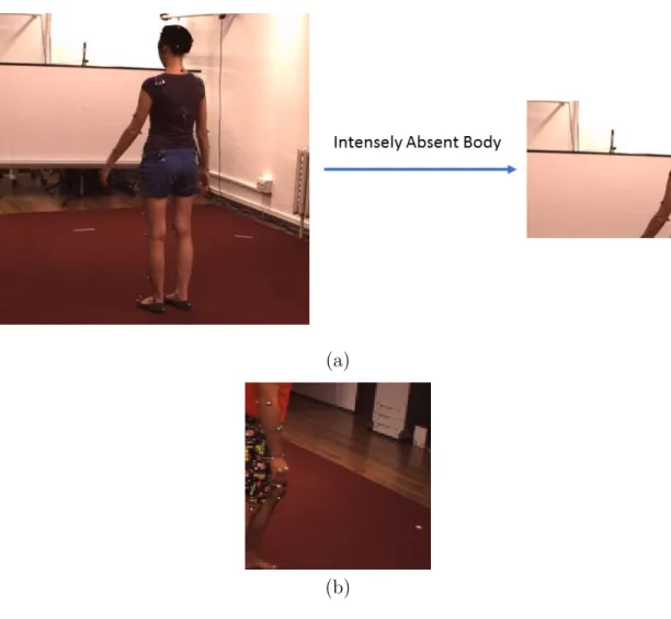
4 Examples of intensely absent pose information. . . 6
5 Human body’s main joints example. . . 10
6 Multiple-input artificial neuron . . . 14
7 Plots of three common activation functionsf(n). . . 14
8 An example of a multilayer fully-connected feedforward neural network 15 9 An example of a two-layer feedforward neural network. . . 17
10 An example of 2×2 max-pooling process. . . 20
11 An example of a CNN . . . 21
12 The block diagram of VNect method [1]. . . 28
13 The block diagram of InWild method [2]. . . 28 14 The proposed 2D pose regression network. All of the convolutional
layers are followed by a Rectified Linear Unit (ReLU). MP indicates a 2x2 max-pooling layer. The dense (fully-connected feedforward) layers at the end of the network are followed by a linear activation function. 31 15 Proposed 2D pose to 3D pose mapping network; each of the dense
16 An overview of the proposed method. . . 34
17 The 3D pose regression network; All of the convolutional layers are followed by a Rectified Linear Unit (ReLU); the dense layers at the end of the network are followed by a linear activation function. MP indicates a 2x2 max-pooling layer. . . 35
18 The proposed detection network. The convolutional layers are followed by a Rectified Linear Unit (ReLU). MP indicates a 2x2 max-pooling layer. The feedforward layer is followed by a softmax activation function. 36 19 Joint regression and detection network. . . 39
20 Example of our random window selection method: (a) an original im-age from the dataset; (b) imim-age with perfectly segmented subject; (c) a randomly selected window. . . 43
21 The main body joints used in this work. . . 44
22 The process of joints’ existence vector generation. . . 45
23 Estimation of learning rates for separate and joint training. . . 49
24 Subjective results under partial body presence. . . 50
25 Subjective results of our method (Part3D) under full body presence. . 58
26 Subjective results of our method (Part3D) under partial body presence for subject 9 of the Human3.6M dataset. . . 59
27 Subjective results of our method (Part3D) under partial body presence for subject 11 of the Human3.6M dataset. . . 60
28 Average of full pose estimation from full body presence and partial pose estimation from partial body presence for different scenarios using direct pose estimation with separate training(Part3Ds). . . 61
29 An example of not-sufficient partial body presence that causes our method to not detect orientation. . . 61
List of Tables
1 List of human body’s main joints; the joints’ numbering follows the indexes in Figure 21. . . 52 2 Overview of joints’ regression stage on Human3.6M dataset measured
on the whole dataset for all tested methods (mean-per-joint-error in mm). Lowest error is bold and second lowest underlined. . . 53 3 Average mean-per-joint-error of full body pose estimation based on
full body images from Human3.6M dataset in mm. Lowest error is bold and second lowest underlined. . . 54 4 Average mean-per-joint-error of full body pose estimation based on
partial input imagesfrom Human3.6M dataset in mm. Lowest error is bold and second lowest underlined. . . 55 5 Average mean-per-joint-error of partial body poseestimation based
on partial input images from Human3.6M dataset in mm. Lowest error is bold and second lowest underlined. . . 56 6 Results of joints’ detection stage on Human3.6M dataset measured
Chapter 1
Introduction
1.1
Motivation
The purpose of 3D human pose estimation is to enable computers to estimate (recon-struct) 3D human poses while being fed with 2D imagery [3]. Reconstruction of the 3D human poses from 2D imagery is a prominent field of research in computer vision [1, 2, 4, 3]. Applications include human-computer interaction, virtual and augmented reality, and robotics. In spite of the vast study of the subject in the literature, it is still assumed a challenging problem. This stems from the inherent loss of the depth information in the 2D images and from image related factors such as blur, noise, occlusion, etc.
3D pose estimation from 2D images is less challenging while using depth images captured by the depth sensors. Depth sensors render another channel pertaining to the distance of the object from the camera aperture; that is, in the rendered images, there exists some information representing the depth of the objects. On the other hand, 2D images do not contain any explicit depth information. Such images provide information on the intensity of the channels (grayscale, RGB, etc.) illustrating the 2D scenery.
(a)2Dimages
(b)2Dposes
Figure1: Twodifferentinputtypesof3Dhumanposeestimation.
TheHumanVisualSystem(HVS)canperceivedepthfrom2Dimagescombining eitherstereoormonocularclues[5]. Despitetheabsenceofexplicitdepthinformation in2Dimages,the HVSisnotfullyimpairedofestimatingthe3Dgeometrywhile havingasingleviewofanobject.ThisperceptionoriginatesfromtheabilityofHVS totakeadvantageofthevisual memoryofobjectshapes[6]. ConsideringFigure1 (a)asanexample,theHVScanhaveanunderstandingofthe3Dhumanposebyjust lookingatasingleview2Dimage.
1
.2 Prob
lemStatement
Theproblemof3Dhumanposeestimationconsistsoftwodifferentformulationsin termsofinput,whichcaneitherbea2Dimageora2Dposeassumedtobeavailable, e.g.,extractedusing2Dposeestimationtechniques. Figure1illustratesthesetwo types.
3D human pose estimation has been previously studied while assuming the full presence of the body parts in the input image. Full body presence means the full shaped human body is present in the image. Here, self-occlusion is excluded, since in these cases, the body is not partially present and the full shape of the body is present to the camera. Partial body presence means the body is partially present in the input image. This can be due to zoom-in photography, imperfect object (bounding box) segmentation, occlusion, or when the whole skeleton of the subject is not aimed to be reconstructed (see Figure 2). Figure 3 (a) shows a case of full body presence, while Figure 3 (b) and (c) illustrate two cases of partial body presence. An example of partial body presence where the whole subject body is not aimed to be reconstructed is when somebody is communicating through video call (see Figure 2 (c)) where the person is often filming oneself in the upper body parts (but not necessarily all of them).
Assuming the need for 3D human pose estimation (e.g., to be used in augmented reality), 3D pose estimators should be able to reconstruct the partial body pose from this partial presence of the body parts. State-of-the-art assume the full presence of the human body and thus do not have effective performance under these cases. Figure 3 (d-f) show the performance of the well-known VNect method [1] applied to the images in Figure 3 (a-c); while going from Figure 3 (a) to (c), the performance is considerably affected. Partial 3D pose estimation under partial body presence can also be viewed as a human pose estimation adaptive to the parts of the body present in the input image and does not make any special assumption about it.
An ability of the HVS is perception of the full body pose when encountering partial body images. An example is when half of the body’s rigid limbs are absent from the input. In this case, the humans’ visual perception’s prior about the rigidity helps reconstruct the full body pose even though some of the body parts are absent.
(a) Zoom-in photography [7] (b) Imperfect Segmentation (c) Video Calling
(d) Occlusion [7] (e) Zoom-in photography [7]
Figure 2: Examples of partial body presence.
For example, by looking at Figure 3 (b), although the ankles are not present in the image, the HVS can perceive the full body pose due to its priors about the rigidity of the legs. State-of-the-art in 3D pose estimation do not estimate 3D full pose under partial body presence.
1.3
Research Objectives
This thesis is concerned with performing 3D pose estimation on a single person from a single view and using a single 2D monocular image, without assuming the existence of 2D poses nor the existence of the full human body in the input image. We assume that the subject is not intensely absent from the image such that significant pose information to recover the body pose is lost, for example, when only the legs or
(a) Full body presence (b) Partial body presence (c) Partial body presence
(d) VNect output for (a) (e) VNect output for (b) (f) VNect output for (d)
Figure 3: Input images with different body parts presence and the output of VNect [1].
pose information, while Figure 3 illustrates examples of sufficient partial presence of the pose information in the input. We design and train a deep neural network (regression network) to regress the full body pose regardless of what joints are present in the input image. We also design a detection stage consisting of detection networks corresponding to each of the main body joints (17 in this work) to classify the presence or absence of the body joints in the fed image. The output of this stage is meant to determine what joints are present in the input image. Thus, our approach to estimate 3D pose under partial body presence consists of two stages: regression and detection, and hence the output of our approach is twofold: the regression network outputs the full pose reconstructed from the input image, and the regression and detection networks output the body pose for the joints present in the input image.
(a)
(b)
Figure 4: Examples of intensely absent pose information.
1.4
Summary of Contributions
The main contribution of this thesis is handling the 3D human pose estimation under partial presence of the body parts. To this end, this work first introduces a method to employ deep neural networks to regress the full human body pose based on input images partially containing the human body. Two different approaches are proposed for this task, namely, using an intermediate 2D pose estimation stage and direct regression of the 3D human pose. Secondly, this work proposes a deep detection stage to classify the presence of each of the joints and provide the body presence
vector. Finally, the detection networks are integrated with the regression network to enable partial estimation of the human pose based on the joints present. Both joint and separate training of the regression and detection networks is proposed and experimented in this work.
1.5
Thesis Outlines
The rest of the thesis is organized as follows. In Chapter 2, we present a review of the background material related to our work. In the first part, we review the basic concepts and mathematical formulation of 3D human pose estimation. In the second part, a review of neural networks is presented as well as deep learning and convolutional neural networks. We also discuss different functionalities of neural networks, i.e., the regression and classification tasks.
In Chapter 3, we present a review of 3D human pose estimation literature. In this chapter, the evolution of 3D human pose estimation is discussed as well as the most related methods to our work.
In Chapter 4, we present the regression network while using a 2D pose estimator as an intermediate task for regressing the 3D pose. This design consists of a 2D pose estimation network followed by a network to extract 3D human pose from the 2D poses. The input to the regression network is a 2D image.
In Chapter 5, we propose a direct 3D human pose estimation architecture using a deep convolutional neural network which is fed with 2D intensity images. This Chapter also presents the architectures used to perform the joints’ detection task. The detection stage is integrated with poses extracted from the regression networks to form the partial output poses. 1
1A paper based on this chapter has been published in IEEE International Conference on Image
In Chapter 6, we present and discuss the experimental setup and the performance evaluation of our method and compare it to the state-of-the-art.
Finally, Chapter 7 concludes this thesis by summarizing the main points and contributions, and giving directions for further work.
Chapter 2
Background Material
2.1
Introduction
In this chapter, we discuss the background material required for our work. In sec-tion 2.2, we discuss the problem of 3D human pose estimasec-tion and its general formu-lations. In section 2.3, the basic concepts of neural networks will be presented with focus on deep learning concepts.
2.2
Formulating 3D human Pose Estimation
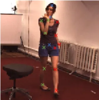
3D human pose estimation is estimating the position of the body’s main joints in the 3D space [3] from 2D images. The body joints are the connections between the bones in a human body. By body’s main joints, we mean the ones which can give us an overall view of the body skeleton (or pose) by connecting the corresponding joints. Figure 5 illustrates presenting the pose using the main body joints. Figure 5 (a) is an example of a human image with highlighted joints locations; cross marks on the figure show the locations of the main body joints. Figure 5 (b) illustrates the corresponding 3D body pose based on the marked joints. Formulations of 3D human
(a) Highlighted joints’ locations (b) 3D body pose based on the marked joints
Figure 5: Human body’s main joints example.
pose estimation differ depending on the input, namely, 2D poses or 2D images. We discuss these two formulations in sections 2.2.1 and 2.2.2, respectively.
2.2.1
3D Human Pose Estimation Using 2D Pose
The 2D human body pose can be defined as the projection of the 3D pose to the image plane [9]. The 2D pose practically illustrates the spatial position of the body joints on the 2D image. AssumingJ the number of main body joints, the 2D human pose matrix W ∈ R2×J is a 2-dimensional matrix in which each column represents
the 2D Cartesian coordinates (x and y) for one of the J main body joints [6, 10, 11]. By defining S ∈ R3×J as the 3D human pose matrix in which each column
rep-resents the 3D Cartesian coordinates (x, y, and z) for one of the j main body joints, the 3D human pose estimation problem can be formulated as a transformation T which maps the 2D joints’ coordinates to their corresponding 3D coordinates in the 3D space. Therefore, the estimation of 3D human body pose based on 2D poses can be basically formulated as
Different approaches can be employed to obtain the transformation T. One of the widely-used approaches is minimization of the reprojection error,e.g., in [6]. In this approach, different projection models may be adopted. Assuming a linear projec-tion between the 2D and 3D poses and Π ∈ R2×3 as the camera calibration matrix projecting the 3D pose to the 2D space, the relationship between the 2D and 3D poses can be stated as
W=ΠS. (2)
The reprojection error is defined as the difference between the actual 2D poses and the 2D poses extracted by projecting the 3D poses to the 2D space
e =d(W,ΠS), (3)
where d is a distance measure (e.g., mean squared error) and e is the reprojection error. Therefore, the 3D human pose estimation can be formulated as the following optimization problem
min
Π,S d(W,ΠS), (4)
which jointly searches for the best camera calibration matrix Π and 3D pose based upon minimization of the reprojection error in (3). The cost function (reprojection error) ein (3) is usually simplified to limit the searching domain by making assump-tions on the projection type (such as using the weak-perspective camera model in [6]).
of some basis shapes S= K X i=1 ciBi, (5)
where Bi is one of the K basis shapes and ci is the corresponding weight. This
approach stems from the active shape model [12]. To model the complex variations more effectively, some methods use sparse representation [2, 6, 13], where an over-complete dictionary is adopted andSis expressed as a sparse combination of the basis shapes from the basis shapes’ dictionary. The cardinality term (or similar terms) is added to the cost function which represents the sum of the weights. This term regularizes the growth of the weights to address the sparseness of the pose model.
Another widely-used approach for extracting 3D pose estimation from 2D poses is using discriminative learning approaches. In these methods, a learning-based mapping between the 2D and 3D poses are learned (e.g., using neural networks) and then it can be used to make estimations about new queries. In this case, the discriminative mapping accounts for the transformation T in (1).
2.2.2
3D Human Pose Estimation Using 2D Imagery
A digital image I(x, y) is represented by its gray levels of intensity (I) or its color components. The image signal is a function of its spatial coordinates in the 2D space (xand y) where the domain depends on the image size. A color image is represented by three components, the most important of which are RGB (red, green, and blue) and HSV (hue, saturation, and value) representations. The gray levels and the color components are usually presented by a number in the (0,2b) range, where b is the
number of bits used to store each of the image pixels (typically b = 8).
as
S=T {I}, (6)
whereT is the transformation from the 2D imagery to 3D human poses andS∈R3×J
is the estimated human body pose in the 3D space. There exist different approaches for modeling the transformation T. One approach is to first extract the 2D human body pose matrix W ∈R2×J using some 2D human pose estimation technique (e.g.,
discriminative methods) and then, the problem follows the discussions in section 2.2.1 (see [11]). Another approach is to view this problem as a discriminative mapping between the 2D images and the 3D poses. In this case, poses are directly regressed from 2D input images [15, 16].
2.3
Artificial Neural Networks
2.3.1
Neurons
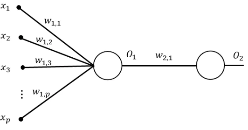
Artificial neurons are the basic building blocks of artificial neural networks [17]. They are inspired by biological neurons in humans’ and animals’ brains which learn struc-tures by being exposed to different sorts of examples and experiences. Figure 6 illustrates a multiple-input artificial neuron. The input-output relationship for this neuron can be written [17] as
y =f(n) = f(
p
X
i=1
w1,ixi+b) = f(Wx+b), (7)
whereyis the output of the neuron,f is the activation function,bis the bias parame-ter, Wis the weights’ vector, and xis the input vector while assuming the neuron to havep inputs. As can be seen in Figure 6, a weighted sum of the inputs (whereW1,i
Figure 6: Multiple-input artificial neuron
is the weight forith inputx
i) is added to a bias term b. In the figure, the value ”1” is
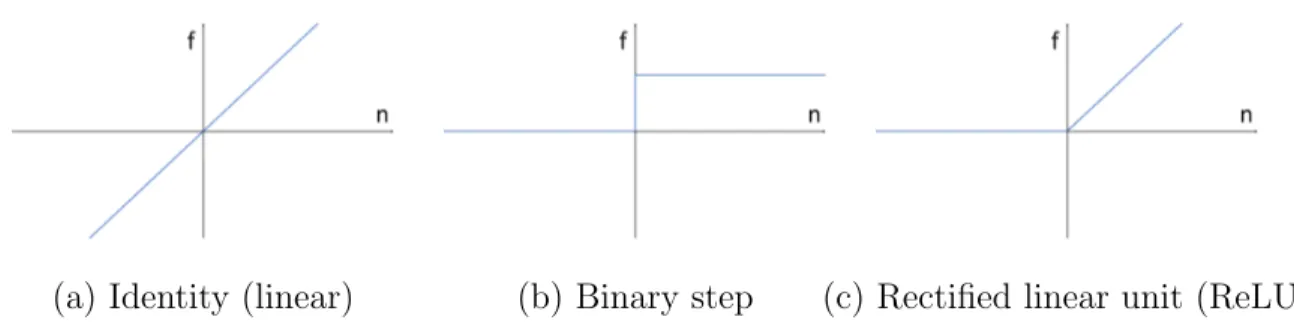
the identity element so that the bias term is simply added to the weighted sum of the inputs. Then, an activation function f takes effect on this summation which results in the output y. W and b are adjustable parameters which give learning capacity to the network and the activation function (also called transfer function) is a specific mathematical linear or non-linear function chosen based on the specifications of the problem. Some of the most common activation functions are the identity (linear), binary step, and rectified linear unit functions; these functions are plotted in Figure 7 (a)-(c), respectively.
(a) Identity (linear) (b) Binary step (c) Rectified linear unit (ReLU)
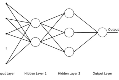
Figure 8: An example of a multilayer fully-connected feedforward neural network
2.3.2
Multilayer Neural Networks
Neurons can be grouped together to form networks representing more complex models [18]. Figure 8 illustrates a fully-connected feedforward neural network. Each circle in this figure represents a single multiple-input artificial neuron (node) as in Figure 6. This neural network is called a feedforward neural network since each of its neurons is only connected to neurons from the previous layers (connections between neurons do not make a cycle). It is also fully-connected as each of the neurons is connected to all of the neurons from the previous layer. The architecture of the network (number of layers and nodes and the way they are connected) is determined by the application and the learning capacity we need. Adding more neurons and layers to the neural network increases the trainable parameters of the network which may help the learning capacity provided that we have enough data to train the network.
2.3.3
Neural Networks’ Learning
Learning in the neural networks can be defined as utilizing a set of pre-verified data to update the model so that the network’s output gets improved, i.e., approaches
an optimal result. More intuitively, a neural network is learning as the adjustable parameters of the network (weights and biases) are updated resulting in less error in the output of the network [17].
A neural network is usually discriminatively trained using the backpropagation al-gorithm [19]. The first step in the backpropagation algorithm is determining the cost (loss) function of the network. The cost function depends on the network architec-ture, activation function, and the type of error chosen for the training stage (based on the task). Mean squared error and cross-entropy are two examples of the most com-mon error functions. After determining the cost function, the neurons’ parameters are initialized which can be done using different techniques, e.g., generating random values for the parameters. The parameters are then iteratively updated using gradi-ent methods in which the weights are updated so that the cost function approaches its local minimum [17]. An iteration is defined as performing backpropagation on a single data point and backpropagating the error once on the whole training data is called an epoch. The idea in gradient methods is to modify the parameters in the opposite direction of the gradient of the output. This approach helps the network update itself so that the value of the cost function is decreased after each iteration. A convex cost function C approaches the global minimum using gradient methods. Us-ing the gradient (steepest) descent method, each of the model weights can be updated using
wnewi,j =wi,jold+ ∆woldi,j =woldi,j −α ∂C ∂wold
i,j
, (8)
wherewi,j is the weight parameter for theith layer and thejth node, αis the learning
rate, and C is the cost function. Decreasing the gradient of the cost function from the weights helps update the weights so that the loss is decreased in each iteration.
Figure 9: An example of a two-layer feedforward neural network.
network parameters are updated. A large learning rate can make the learning process unstable since the large steps in the cost function can result in overshooting the minimum, and thus even not converging to the optimal solution. Small learning rates mean slower learning speed, and thus the convergence time may be increased. Another solution for determination of the learning rate is to start with large learning rates and then decreasing it as we approach the minimum. Therefore, different functions (which can depend on the number of iterations) can be used for the learning rate, e.g., dividing the learning rate by a value after each iteration (or a group of iterations).
The weights for the hidden layers are updated using thechain rule from calculus. To explain the chain rule in training the neural networks, we assume a network with 2 layers (1 hidden layer and 1 output layer) as shown in Figure 9. Assuming each of the layers having a single neuron, C the cost function, O2 the output of the output layer, O1 the output of the hidden layer, and w1,i the weight for the ith input, the
partial derivative of the cost function with respect to this weight is
∂C ∂w1,i = ∂C ∂O2 × ∂O2 ∂O1 × ∂O1 ∂w1,i . (9)
Thus, this weight can be updated in each iteration using w1new,i =wold1,i −α ∂C ∂O2 × ∂O2 ∂O1 × ∂O1 ∂w1,i . (10)
ADAM [20] is one of the widely used optimization methods for backpropagating the gradient errors in neural networks, due to its time and memory efficiency. ADAM method selects separate learning rates for different network parameters based on an estimation of the first and second moments of the gradients.
2.3.4
Deep Learning
Deep learning methods use models with multiple processing layers each of which correspond to different levels of abstraction [21]. More intuitively, the idea in deep neural networks is to use features extracted by each of the layers (which can be viewed as a level of abstracting the information) as the input to another neural layer so that we can have higher levels of abstraction. These features differ based on the application.
In practice, deep neural networks have more than a single layer [22]. These net-works are trained to find a discriminative representation of the data. The types of layers in deep neural networks can differ based on the application. Some of the most famous layer types are feedforward, convolutional, and recurrent neural layers. Using these layers, different network types are designed based on the application, where convolutional neural networks (CNNs) are widely used in computer vision.
2.3.5
Convolutional Neural Networks
Convolutional neural networks (CNNs) are designed for processing the data coming in the form of multiple arrays, and thus are appropriate choices for dealing with image
data [21]. CNNs take advantage of a number of layer types making them a great fit for many computer vision applications. We introduce the main CNN layer types, namely, Convolutional and Pooling layers, briefly in the following.
2.3.5.1 Layer Types
Convolutional Layers: a convolutional layer consists of a set of trainable parame-ters (weights) which are called filter banks. The filter banks do not change spatially and are kept the same for all inputs of each layer (pixels in 2D images, features in higher layers). Convolutional layers apply a convolution operation between the input of the layer and the filter bank. The convolution operation helps extract features from the input benefiting from local conjunctions of the features in any neighborhood of the pixels. The feature extraction process directly applied on an image (first layer) can be considered as a sort of edge detection. In the rest of the layers, the extracted features correspond to higher levels of abstraction. Sharing the weights (using the same filter bank for all the inputs of each layer) helps making the extracted features invariant to position.
The output of the convolution operation is then passed to an activation func-tion. A widely-used example of the activation functions is the Rectified Linear Units
(ReLUs) expressed as
f(x) =max(0, x), (11)
wherexis the input to the function andf(x) is the output of the ReLU function (see Figure 7 (c)).
When the input to the first layer is a 2D image, the output features are edge-related as they are weighted summation of input pixels. Features in next layers are extracted by the convolutional layer itself and are not necessarily known to human
Figure 10: An example of 2×2 max-pooling process. perception.
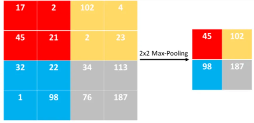
Pooling Layers: a pooling layer merges semantically relevant features into one. Max-pooling layers are one of the most popular pooling layers which calculate the maximum of the pixels’ intensities in a local patch of a feature map (e.g., input image or output of any of the convolutional layers). For example, considering a 2×2 max-pooling layer, for any 2×2 patch of the input, the maximum value is kept to represent the whole patch. Therefore, the input will be downsized by a factor of 2 in each direction. Figure 10 illustrates the process of 2×2 max-pooling layer.
2.3.5.2 CNN Design
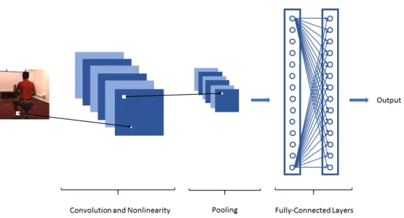
CNNs are usually formed by cascading a few number of convolutional (usually followed by a nonlinear activation function such as ReLU) and pooling layers. They are then followed by fully-connected neural networks (also called dense layers). This network can be then trained by backpropagating the cost function gradients such that all the weights are trained. Figure 11 illustrates an example of a CNN architecture with one convolutional layer, one pooling layer, and two fully-connected layers. Different CNN architectures can be designed using the explained layers depending on the application.
Figure 11: An example of a CNN
of CNNs. One of these methods is batch normalization [23]. In training CNNs, the data is usually fed to the network in groups of data points which are called batches. The batch size represents the number of data points (images in this work) which are fed jointly to the network and it is a hyper-parameter chosen based on the available computational capacity. In batch normalization, any batch is normalized before being fed to the fully-connected neural layer to prevent change of the input distribution in the middle of the training process.
Another useful method to enhance the performance of the CNNs is randomdropout
of the feature detectors (network parameters) [24]. For example, in a 0.5 dropout, half of the parameters are randomly removed in each training case. This method -especially when dealing with small-size datasets - can reduce the possibility of the
overfitting problem by a great amount. Overfitting is a major problem in the learning process while dealing with small datasets. In overfitting, the network - especially when the network capacity is high - is so vulnerable to learning the data too closely that
the learning process can be considered as a sort of memorization. Thus, overfitting can prevent the network from performing the generalization task effectively.
2.3.5.3 CNN Tasks
The task, for which a CNN is designed, is a dominant factor in the architecture design of the network. The main two classes of tasks in CNNs are classification and
regression tasks.
Classification: In this set of problems, the network’s output is a label which is chosen among a limited set of possible outcomes (classes). Image classification is an example of this task, where a limited number of image classes exists; therefore, any image is assumed to belong to one of these classes. Detection problems are another example of the classification task in which the output can take only two values, namely, ”detected” and ”not detected”. Classification problems with 2 possible labels are called binary classification problems.
Regression: Regression is the analysis of a quantity of interest using the informa-tion from one or more other quantities [25]. In regression problems, the network is designed to predict a real quantity (a continuous value). An example of the regression task is depth estimation [26, 27] where the input is an image and the objective is to estimate the depth values for each of the pixels. This depth is a continuous value, i.e., it is not chosen among a limited set of possible outcomes and can take any value in the valid range (e.g., positive values in depth estimation). Precipitation prediction
[28] is another example of the regression task; these problems are categorized as a regression task since the output (precipitation amount) is a continuous quantity.
Chapter 3
Literature Review
3.1
Introduction
Techniques to human pose estimation [3] have various forms ranging from pose es-timation for a specific part of the human body to the full body pose eses-timation (e.g.[1, 4, 2]). Pose estimation of specific human body parts includes hand pose es-timation [29, 30, 31, 32], head pose eses-timation [33, 34, 35, 36], and upper-body pose estimation [37].
Human pose estimation techniques can be categorized into 2D and 3D pose es-timation in terms of the dimensionality of the output. 2D pose eses-timation aims to find the location of the main body joints on the image plane, i.e., determining the pixel with the most probability of being the location of some specific body joint. 2D human pose estimation has been well studied (e.g., [4, 10, 38, 39, 40, 41, 42]). 3D pose estimation is an active research field [1, 2, 6, 11, 13] but remains challenging due to the ambiguity caused by the loss of depth information in the usual intensity images but also due to image related issues such as blur, noise, occlusion, etc. Some meth-ods use depth images containing explicit depth information for 3D pose estimation [43, 44, 45, 46].
The remaining of this chapter is organized as follows. In section 3.2, we discuss the problem of structure from motion; section 3.3 summarizes literature of 3D human pose estimation and section 3.4 highlights one of the widely-used approaches, namely, the discriminative deep learning approach.
3.2
Structure from Motion Methods
Historically, the idea of extracting 3D structures from 2D imagery has been vastly studied under structure-from-motion (SfM) [47, 48]. SfM is often focused on mapping 2D key points or features to the 3D space. SfM usually follows a 2D key point detection or feature extraction stage. Some of the well-known feature extraction methods are scale-invariant feature transform (SIFT) [49, 50] and speeded-up robust features (SURF) [51].
Tomasi and Kanade in [47] develop a factorization method based on the decom-position of the input data (2D keypoints/feature) into two different matrices; one of these matrices correspond to the motion parameters and the other one to the 3D structure. In [47], the object is assumed to be rigid. Bregler et al. [48] generalize this method to deformable shapes assuming the deformable shapes as a linear combination of some basis rigid shapes.
Another class of relevant topics to human pose estimation is objects’ pose esti-mation and tracking [52] which is usually formulated as matching some key points or features in a target image with those in new queries (input images). Zhou et al. [6] present a 3D car model estimation using 2D annotations as well as 3D human pose estimation.
3.3
3D Human Pose Estimation Methods
3D human pose estimation outputs an estimate of joints’ 3D positions (or the angles) using 2D information, which is usually given in terms of either 2D images or joints’ 2D locations (2D pose). 3D pose estimation methods based on 2D joints’ location assume that the 2D joints have been given or already extracted using some 2D pose estimation technique. They use various techniques such as sparse representation[6, 11], factorization [13], and neural networks[53] to estimate the 3D poses from 2D poses. Zhou et al. in [6, 11] propose to use a convex approach while using sparse representation for the 3D human pose estimation from 2D landmarks. The method in [11] presents a 2D joints’ uncertainty map predictor to handle the cases when 2D joints’ information is not available. Wandt et al. [13] try to factorize 2D poses in camera parameters, base 3D human poses, and mixing coefficients. They also show that making periodic assumptions on the mixing coefficients can improve the performance in 3D human pose estimation. Tekin et al. [54] have introduced some method to fuse two different streams, one acting on 2D joints information and the other on the images to extract the 3D pose information. Martinez et al. [53] discuss different natures of the error between the ground truth and estimated poses while having a 3D pose estimator with a 2D pose estimator as an intermediate stage; that is, they compare the results while extracting the 3D pose directly from the ground truth 2D poses and while regressing the 3D pose from 2D poses extracted by some off-the-shelf 2D pose estimation techniques.
3D pose estimation methods directly from 2D images can be categorized to those using a single view for the estimations [55] and those leveraging multi-view imagery[37, 56, 57]. Single-view methods are used for cases in which there is only a single camera capturing image or video from the scene, and thus its view is the only present in-formation to estimate the 3D pose. In these methods, even when using the datasets
providing the data from different viewpoints, frames from each viewpoint are consid-ered as separate data points and each frame is treated as an individual single-view image. On the other hand, in multi-view cases, there are a few cameras filming from different viewpoints. The cases consisting of multi-view are easier to extract the depth information since, in the single-view, there is more loss of the depth information in the captured imagery.
3D pose estimation techniques can also be categorized into those estimating the pose assuming a single person present in the window (e.g., [58]) and those doing the estimation for multiple people [57].
Another important classification of direct 3D pose estimation methods is those performing the estimation on a single image(e.g.[15, 55]) as opposed to the ones per-forming on a sequence of images (video) [11, 14]. Zhou et al. [11] use an expectation-Maximization algorithm on the whole image sequence. They add a temporal smooth-ness prior to the penalty (cost) function to take advantage of the existing information over time. Tekin et al. [14] compensate for the motion to keep the subject centered and then regress the 3D pose in the central frame directly from a spatiotemporal volume of bounding boxes.
Another classification of human pose estimation methods is generative and dis-criminative approaches. Generative approaches use some a priori information to per-form the estimation and thus include a modeling stage in advance to extracting the 3D poses[59]. An example of these priors is the size of each of the body parts and their topology as used in [59]. Discriminative approaches are the data-driven model-free methods which learn a mapping between the input images (also features or 2D poses) and the desired output(e.g.[15, 55, 60, 61]). The method in [60] leverages a large database of 3D human motion capture combined with a human model from 3D computer graphics to generate training pairs of 3D human pose with their realistic
2D silhouettes. Ning et al. in [61] use the bag of (visual) words approach to discrim-inatively estimate 3D pose from a 2D image. Deep learning approaches are another category of discriminative approaches which have been widely used in 3D human pose estimation.
3.4
Discriminative Deep Learning Approaches
Deep learning is a general concept for learning data representation using deep multi-layer networks [21] which has drawn significant attention since its early introduction. Numerous papers have utilized deep learning concepts to address the problem of 3D human pose estimation[1, 2, 11, 15, 16, 55, 58]. Among these methods, some perform an initial 2D pose estimation stage and then use that information to estimate the 3D pose[11]. Mehta et al. [1] use 2D pose estimation to locate the subject and thus do not need tightly cropped windows. Some deep learning methods [15, 16] perform direct estimation of the 3D poses without any need to regress the 2D pose in advance. Brau and Jiang [58] perform direct regression of the 3D poses; however, they add a 2D projection layer to enforce pose constraints on the estimated output. Pavlakos et al. [55] handle the estimation by discretization of the 3D space and regressing per-voxel likelihood for the joints in the discrete 3D space.
3.5
Most Related Work
To the best knowledge of the author, no publication exists that handles 3D human pose estimation from 2D images under partial body presence. In this section, we discuss methods most related to ours. The method [62] estimates the pose partially; however, it is based on depth sensors and not monocular 2D imagery. The method in [16] has a detection network as a pre-training stage; however, it still does not take
into account partial body presence. It also performs joint training of the detection and regression networks. The detection stage in this work is not the same as ours in the sense that [16] detects the presence of joints concerning whether or not they encounter self-occlusion (and not partial body presence as defined in this work).
The methods VNect by Mehta et al. [1] and InWild by Zhou et al. [2] do not take into account partial body presence; however, they are close to our work as they perform 3D human pose estimation directly from 2D images using deep CNNs. VNect method [1] uses a CNN architecture combined with kinematic skeleton fitting to regress 2D and 3D joints’ locations, jointly; see Figure 12. InWild method [2] cascades a 2D regression network with a 3D depth regression network to extract the 3D human pose from 2D images; as shown in Figure 13.
Figure 12: The block diagram of VNect method [1].
Chapter 4
3D Pose Regression Based on 2D
Pose Regression from Partial Body
Images
4.1
Introduction
In this chapter, we present our first approach to regress the 3D human pose from a 2D image using 2D pose regression as an intermediate stage under partial body (Part2D3D). In this approach, the image is primarily fed to a CNN to regress the 2D joints’ locations directly from the input images. The following step is to map the 2D poses to the corresponding 3D poses.
The rest of this chapter is organized as follows: in section 4.2, we present the architecture used in our network to perform the regression; then, section 4.3 presents the training details of our method.
4.2
Proposed Network Architecture
The network architecture in our approach contains two separate networks used for the two different stages of the 3D pose regression, namely, extracting the 2D poses and mapping the 2D poses with the corresponding 3D poses. These networks will be presented in sections 4.2.1 and 4.2.2, respectively
4.2.1
2D Pose Estimation
We perform 2D pose estimation by direct discriminative regression of 2D poses from 2D input images using CNNs. The used CNN is illustrated in Figure 14, where the input is a single 2D intensity image and the output is 2D human pose, which is a matrix showing the position of the body’s main joints using 2D Cartesian coordinates. The network consists of five convolutional layers with kernel sizes of 9×9, 9×9, 5×5, 3×3, and 3×3. The depths of these layers are 128, 256, 256, 128, and 64, respectively. It also contains three max-pooling layers each of which downsize the input features by the factor of 2×2. Each of these layers is followed by a batch normalization and a rectified linear unit. Then, we have two layers of fully-connected feedforward (dense) layers with 4096 neurons, each followed by a 0.5 dropout and a linear activation function.
The output of this network is normalized by dividing the 2D coordinates by the width and height of the input image size (both equal to 150 in this work since the input to our network is a 150×150 image). This normalization is done on the ground truth 2D poses since we want this network to address 2D pose estimation for partial cases. In other words, in this step, we assume to have a (hypothetical) full body image, and we try to extract its (full) 2D pose from the partial body input. Therefore, although this output has the same nature as 2D human pose, it is not exactly meant
Figure14: Theproposed2Dposeregressionnetwork. Alloftheconvolutionallayers arefollowedbya RectifiedLinear Unit(ReLU). MPindicatesa2x2 max-pooling layer. Thedense(fully-connectedfeedforward)layersattheendofthenetworkare followedbyalinearactivationfunction.
full2Dpose(inwhicheachofthecoordinatesisanumberbetween0and1),generated to makeabasisforextractionof3Dhumanposeinformation.
4
.2
.2 2D Poseto3D Pose Mapp
ing
The mappingfrom2Dposesto3Dposesisperformedusingaful ly-connectedfeed-forwardneuralnetwork.Theinputtothisnetworkisthenormalized2Dposeandthe outputisthe3Dhumanpose. Thisnetworkis meanttolearndifferentbodyposes byencounteringdifferentscenarios. Thearchitectureconsistsoftwofully-connected (dense)layersofsize2048. Figure15illustratestheproposed2Dposeto3Dpose mappingstage. EachofthelayersarefollowedbyaReLUactivationfunction. We useda0.5dropoutoneachlayertopreventoverfitting.
4
.3 Tra
in
ing Deta
i
ls
Thelossfunctionusedfortrainingthenetworksisthemeansquarederror MSE(ygt,yest)=1 DJ J k1=1 D k2=1 (ygt k1,k2−y est k1,k2)2, (12)
Figure15:Proposed2Dposeto3Dpose mappingnetwork;eachofthedenselayers arefollowedbyaReLUanda0.5dropout.
whereygtandyestareJ×Dmatricescontaining,respectively,thegroundtruthsand
estimatedvaluesofthebodyjoints’locations.Inthesematrices,eachrowrepresents theCartesiancoordinatesofoneofthebody’s mainjoints.Jisthetotalnumber ofbody’s mainjointsandD isthedimensionalityofthecoordinateswhichequals2 forthe2Dextractionnetworkandequals3forthe2Dto3D mappingnetwork. The networksaretrainedusingADAMoptimization[20]withalearningrateof0.0001
Wefeedthenetworkwithfullandpartialbodyimages. To makesurethatthe networkiseffectivelytrained,soto maintainthehumanbodystructure,weprovide thenetworkwiththefullposes(2Dposesastheoutputofour2Dposeestimatorand 3Dposesfrom mapping2Dto3Dposes). Therefore,allthedatathatispresented tothenetworkrespectsthehumanbodystructure,i.e.,theyarethefullposeofthe humanbodywhetherornotitisfullypresentintheinputimage.Inotherwords, thenetworkistrainedusingbothcasesofpartialandfullbodypresenceastheinput whilehavingthefullbodyposefedasthegroundtruthforbothofthecases.
ExperimentalsetupandsimulationresultsofourapproachPart2D3D,i.e.,3D poseestimationusing2DposeestimationarepresentedanddiscussedinChapter6.
Chapter 5
Direct 3D Pose Estimation from
Partial Body Images
5.1
Introduction
In this chapter, we present our method for direct estimation of 3D human poses under partial body presence (Part3D). It consists of a regression CNN network to regress the 3D human pose directly from 2D input images under partial body presence and a detection CNN network to detect the joints present in the input image. Figure 16 illustrates an overview of our proposed method having two different outputs. The first output is the 3D full body pose extracted by the regression network, where the input image can contain the body parts either fully or partially. The second output is the 3D partial body pose generated by integrating the regression and detection networks. As the detection networks are meant to determine the joints present in the input image, this output is the partial pose resulting from the 3D location of the joints present in the input image.
The rest of this chapter is organized as follows: in section 5.2, we present the architectures used in our regression and detection networks; then, section 5.3 presents
Figure16: Anoverviewoftheproposed method. thetrainingdetailsofour method.
5
.2 Network Arch
itecture
5
.2
.1 Regress
ion Network
’s Arch
itecture
Theproposedregressionnetworkregressesthebody’sjoints’locationsinthe3Dspace forallthejoints-regardlessofwhetherornotitisfedwithanimagecontainingthe fullsubjectbody. Figure17illustratestheCNNsusedfortheregressionstage. As seen,thenetwork’sinputisa3-channelimage. Theinputimageisfirstresizedto 150×150. Theinputisthenfedtotheconvolutionallayers. Ourregressionnetwork consistsoffiveconvolutionallayersandtwofully-connectedfeedforwardlayers,the detailsofwhichareasfollows.
Layer1: thislayerconsistsofaconvolutionallayerofsize128witha9×9kernel followedbyaRectifiedLinearUnitastheactivationfunction.
Figure17:The3Dposeregressionnetwork;Alloftheconvolutionallayersarefollowed byaRectifiedLinearUnit(ReLU);thedenselayersattheendofthenetworkare followedbyalinearactivationfunction. MPindicatesa2x2 max-poolinglayer. activationfunctionistheRectifiedLinearUnitandisfollowedbya2×2max-pooling layerwhichresizestheoutputfeaturesfrom150×150to75×75.
Layer3: thislayerconsistsofaconvolutionallayerofsize256witha5×5kernel andaRectifiedLinearUnitactivationfunction,followedbya2×2max-poolinglayer whichresizestheoutputfeaturesfrom75×75to37×37.
Layer4: thislayerisaconvolutionallayerofsize128witha3×3kernel,anda RectifiedLinearUnitactivationfunction,followedbya2×2max-poolinglayerwhich resizestheoutputfeaturesfrom37×37to18×18.
Layer5:thislayerisaconvolutionallayerofsize64witha3×3kernel,followedby RectifiedLinearUnitastheactivationfunction.
Layer6: thisisafully-connectedfeedforwardlayerofsize4096thatisfed with featuresextractedbythe5thlayerafterbeingflattened,i.e.,theoutputoftheprevious
layerisconcatenatedandconvertedtoavector.Theactivationfunctionofthislayer isalinearactivationfunction.
Layer7:thisisafully-connectedfeedforwardlayerofsize4096;itsoutputisavector ofsize51whichpresentsthepredicted3Dlocationsofhumanbody’smain17joints. Itisfollowedbyalinearactivationfunction.
Alloftheconvolutionallayersarefollowedbyabatchnormalizationlayerto increasethestabilityofthelearningprocess.Eachofthefeedforwardlayersisfollowed
bya0.5dropoutregularizationtopreventoverfitting.
5
.2
.2 Detect
ion Networks
’ Arch
itecture
Theproposeddetectionstageclassifiesthepresenceorabsenceofeachofthehuman body’s mainjoints.Itsoutputisabinaryvectorofsize17indicatingpresenceor absenceofthejointsintheinputimage. Thedetectionstageincludes17detection networks,eachofwhichclassifiesthepresenceorabsenceofoneof17 mainbody joints. Figure18illustratesthenetworkarchitectureforeachofthe17detection networks. Asseen,adetectionnetworkconsistsof2convolutionallayersandone fully-connectedfeedforwardlayerasfollows,wheretheinputisa2Dinputimage.
Figure18: Theproposeddetectionnetwork. Theconvolutionallayersarefollowed bya RectifiedLinear Unit(ReLU). MPindicatesa2x2 max-poolinglayer. The feedforwardlayerisfollowedbyasoftmaxactivationfunction.
Layer1: thisisaconvolutionallayerofsize32witha9×9kernel,followedbya RectifiedLinearUnitastheactivationfunction. A2×2 max-poolinglayerfollows whichresizestheoutputfeaturesfrom150×150to75×75.
Layer2: thisisaconvolutionallayerofsize32witha9×9kernel,followedbya RectifiedLinearUnitactivationfunction.Itisfollowedbya2×2max-poolinglayer whichresizestheoutputfeaturesfrom75×75to37×37.
extracted by the 2nd layer after being flattened. The activation function is a softmax
activation function. The softmax function is defined as
f(xi) =
exi
Pk
j=0exj
i= 0,1, ..., k, (13)
where xi is the input of the softmax function, and f is the output. k is the number
of classes which is equal to 2 in this case, where k = 0 represents the ”absent” class and k = 1 represents the ”present” class. Therefore, this layer has a binary output classifying the presence or absence of the corresponding body joint in the input image. Both of the convolutional layers are followed by a batch normalization layer and the feedforward layer is followed by a 0.5 dropout regularization to prevent overfitting; this network is not much prone to overfitting considering its size, however.
5.3
Training Details
We used the mean squared error as in (12) as the loss function of our regression network. The cost function we used for the detection networks is thecross-entropy
CEj =−[θjlog(pj) + (1−θj)log(1−pj)], (14)
where CEj is the cross-entropy for the jth data point (joint), θj is 1 if the joint is
present in the input and 0 if not, and pj is the probability by which the network
has estimated the joint to be present. The optimization technique for the purpose of training the networks is ADAM optimization [20].
We have tested two different approaches to train the regression and detection networks. The first approach is joint training, in which the networks are combined and trained simultaneously. The second approach is to train the networks separately. These two approaches are explained in the following.
5.3.1
Joint Training
In the joint training approach, the regression and detection networks are assumed to be combined together, and thus only a single cost function is defined for the whole network. The cost function is a weighted sum of the individual cost functions. Therefore, the overall cost function of the joint training network Ct is defined as
Ct=αCreg+β J X j=1 Cjdet =αM SE+β J X j=1 CEj (15)
where Creg is the cost function of the regression network (mean squared error) as in
(12), Cdet
j is the cost function of the detection network (cross-entropy) corresponding
to the jth body joint as in (14), and J is the number of main body joints. In this equation, α and β are the cost function weights of the regression and the detection networks in the overall cost function, respectively. α and β are hyper-parameters determining the impact of their corresponding cost functions on the overall cost func-tion. We set α = 1 and β = 0.1, where all the 17 detection networks share the same weight.
We have used the same feature extraction process for the regression and detection networks in this approach; that is, we have kept the convolutional layers for all of the networks and the networks differ only in their fully-connected layers. We used the convolutional layers from the regression network since they are deeper and have more computational capacity. Figure 19 shows the joint regression and detection network. We used a learning rate of 0.0001 (which is set experimentally by trying different values and monitoring the convergence of the network) and a batch size of 32. The weights are initialized randomly, and the data is shuffled before every epoch. By shuffling the data, we mean reorganizing the data points randomly so that they are fed to the network in a different order for every epoch.
Figure19:Jointregressionanddetectionnetwork.
5
.3
.2 Separate Tra
in
ing
Inthisapproach,thedetectionandregressionnetworksaretreatedastwocompletely separatenetworks. Therefore,foreachofthem,thenetworkisinitialized,trained, andfine-tunedseparatelyasanindividualnetwork. Weusedalearningrateof0.0001 forboththeregressionandthedetectionnetwork. Thebatchsizefortheregression network’strainingis32whilethebatchsizeforthedetectionnetworks’trainingis 256. Havinggreaterbatchsizesusuallyhelpsthenetworkconverge morerapidly. However,becauseofthelimitationofthecomputationalinfrastructurewecouldnot usegreaterbatchsizefortheregressionnetwork(notingthattheregressionnetwork has much moretrainableparametersthanthedetectionnetwork). Theweightsare initializedrandomly,andthedataisshuffledbeforeeachepoch.
Theregressionnetworkistrainedbyfeedingthefullposeasthegroundtruth outputofthenetworkwhilegivingbothfullandpartialbodypresencecasesasthe input. Thisapproachisadoptedtoenablethenetworktolearnthewholehuman
body structure and enable the network to make full body estimations (although not accurate for all the body joints) under both the full and partial body presence cases. The experimental setup and the simulation results of our method Part3D for direct estimation of the 3D human pose from a partial body input image are presented and discussed in Chapter 6.
Chapter 6
Experimental Setup and Results
6.1
Introduction
In this Chapter, we provide and discuss the experimental setup and the results of our methods presented in Chapter 4 and 5. In section 6.2, we present the experimental setup for our work; in section 6.3 we discuss the evaluation protocol; then, section 6.4 presents and discusses the simulation results of our methods.
6.2
Experimental Setup
The network architectures have been selected experimentally by evaluating the per-formance of different architectures. We have started with a network having a single convolutional layer as well as a single dense layer. Then, we added more layers (with different depths and kernel sizes) and evaluated the performance of the new network. Each layer was added only if it improves the performance. This process is stopped when a layer either does not improve the network performance or makes the network excessively large such that the training or predicting process gets very slow.
the network architecture design has been performed only for the first network (we started with direct pose estimation with separate training). We started with one convolutional layer and went up until 7 convolutional layers. For other two, we used the same convolutional layers and only tested the network with one more and one less layer to evaluate the effectiveness of our architecture. For the detection network, we tried 1 to 5 convolutional layers. The experimentations showed that having more than 2 layers does not improve the performance considerably; it reduces the efficiency, however, as we have 17 detection networks.
We use the Human3.6M dataset [63] to assess the performance of our methods. The Human3.6M dataset is a widely-used 3D human pose estimation dataset and includes 3.6 million frames in video sequences of frame size 1000 ×1000 on seven subjects, and each subject performs 15 different actions (e.g., Directions, Discussion, and Eating) while being filmed from four different viewpoints. We have used five subjects (i.e., S1, S5, S6, S7, and S8) for training and two subjects (i.e., S9 and S11) for testing. We have assessed our methods on all of the scenarios of the selected subjects.
To provide the networks with partial body images, firstly, we segment the subject in each of the original images using the bounding boxes provided in the dataset; that is, we draw a square region fully covering the subject body. Then we store two different images each of size 150×150: 1) the segmented image which accounts for the full body case and 2) the corresponding partial body version which is generated using arandom window selection approach. Therefore, we have equal size of full and partial body presence cases as the input. In other words, for any full body presence case, there exists a case of partial body presence, both of which share the same subject and 3D full pose. We have used 150×150 input images since using this dimensionality, we did not need to upsample many of the images, and thus we could use input images
(a) (b) (c)
Figure 20: Example of our random window selection method: (a) an original image from the dataset; (b) image with perfectly segmented subject; (c) a randomly selected window.
with the original quality.
To generate partial body images (windows), we use a random window selection, where the top-left and bottom-right corners of the window are selected randomly with a uniform distribution. This is to make sure we have different cases of partial body presence cases generated among our new set of data. To ensure that sufficient joints exist in the input image, i.e., the image is not intensely cropped that it is not possible to extract pose information from the image, the randomly cropped window size must be larger than a quarter of the original image. Figure 20 illustrates an example of this random window selection: Figure 20 (a) is an original image from the dataset, Figure 20 (b) is the square bounding box drawn around the subject, and Figure 20 (c) is an example of a randomly selected window.
For training, using our above-mentioned random selection of windows, we ex-tracted two windows from each of the video frames of the training set in [63] and one window from each of the video frames of the validation (test) set. In total, we have used 623,900 extracted windows for training and 548,819 for testing. The ground truth 3D poses and 2D poses are provided in the dataset. We have downsampled the video frames by a factor of five, before the random window selection, to avoid
Figure 21: The main body joints used in this work.
redundancy in the training and each video frame is treated as an independent data point. The processing time of every epoch on the whole training data using a Titan Xp GPU was approximately 6 hours for the regression network and 30 minutes for the detection networks and the processing time for every new test image in valida-tion stage was approximately 1∼2 seconds for the regression network and less than 1 second for the detection networks.
In this thesis, we assume 17 joints as the main body joints to form the human body pose. Figure 21 shows and indexes the main body joints used in our method and Table 1 lists these joints. One can use the same architecture with different number of the joints, however, since the features extracted for different number of joints do not seem to vary, and thus changing the number of the body joints should not much affect the performance.
existencevector whichisavectorofsize17. Eachoftheelementsofthisvector isabinaryvaluewhichis1ifthecorrespondingjointispresentintheimageand 0ifnot. Thedatasetdoesnotprovidethisdata. Toextractthesebinaryground truthnumbers,weusethedatafrom2Dposegroundtruthwhichareprovidedin thedataset. The2Dposegroundtruthdeterminestheexactlocationofeachof thejointsintheimageplane. Aftereachrandomwindowselection,allthejoints’ coordinatesarecomparedtotheselected windowtoseeifthejointfallsintothe chosenwindow. Usingthiscomparison,the17binaryvaluescorrespondingtothe main17bodyjointsaredeterminedandusedasthegroundtruthtothedetection stage.Figure22illustratestheprocessofjoints’existencevectorgeneration.
Figure22: Theprocessofjoints’existencevectorgeneration.
6
.3 Eva
luat
ion Protoco
l
TheperformanceassessmenttakesplaceonthelasttwosubjectsoftheHuman3.6M dataset(S9andS11)whichweuseforvalidation.Toevaluatetheperformanceofthe
regression stage, we use themean-per-joint-error (expressed in millimeter) L(ygt, yest) = 1 J J X j=1 ||Cjygt−Cjyest||2, (16) where ygt is the ground truth joints’ position matrix, yest is the estimated joints’
position matrix, || · ||2 is the Euclidean norm, C
ygt
j is the vector of thejth column of
the matrix ygt, C yest
j is the vector of the j
th column of the matrix y
est, and J is the
number of the joints (either J = 17 for full body pose or J = J0, where J0 is the number of joints present). The mean-per-joint-error L(·) in (16) is calculated after aligning the root joint (a joint assumed as the reference; pelvis in this work); that is, the locations of the root joints of the ground truth and the estimated poses are aligned. We have calculated L(ygt, yest) both on the full body skeleton (J = 17) and
the joints which are present inside the window (J = J0). These two measurements are used to assess the performance of our methods for the two different outputs; that is, the full body pose estimation and the partial body pose estimation (the joints present in the input image). We present these errors both on the individual scenarios and on the whole dataset.
The detection stage is evaluated separately for each of the body joints. As the evaluation measure, we use thebinary accuracy which is the percentage of the detec-tions in which the presence or absence of the corresponding joint has been successfully detected; this metric can be formulated as:
ACC = N umber of true detections
6.4
Simulation Results
We compare our methods to two of the state-of-the-art, namely, ”VNect” method [1] and the ”InWild” method [2]. The authors provide their trained networks and open-source code for experimentation. Since we need to assess the methods with the data prepared for the partial body presence cases, we need open-source methods for comparison.
6.4.1
Objective Evaluation
To asses the results from the regression task, we present the outputs for our methods as well as their comparison with VNect [1] and InWild [2] methods. The results of our methods are presented for the 3 different approaches used in this work; namely, 3D pose regression using 2D pose estimation (Part2D3D), direct 3D pose estimation with joint training of the regression and detection networks (Part3D), and direct 3D human estimation with separate training (Part3Ds). The outputs to be discussed are the ”full pose estimation from full body presence”, ”full pose estimation from partial body presence”, and ”partial pose estimation from partial body presence”. The results with these three outputs are summarized in Table 2 and detailed based on the 15 scenarios of the Human3.6M dataset in Tables 3, 4, and 5, respectively.
Table 2 summarizes the performance of our and related methods. It shows promis-ing performance of our method compared to related work; our method well recovers part of the joints not present in the input. It is also noteworthy that our three ap-proaches have very close overall performance. This can be interpreted by considering the fact that all three networks have the same architecture in terms of the convolu-tional layers. This causes the networks to have similar feature extraction stages and also their learning capacity to be very close to each other. The difference between them stems from the difference in the nature of their specific training process, where
they take advantage of 2D pose information, 3D pose information, or 3D pose infor-mation as well as joints’ presence data. Considering their difference in Table 2, we can see that, among the three approaches adopted in this work, 3D pose

![Figure 3: Input images with different body parts presence and the output of VNect [1].](https://thumb-us.123doks.com/thumbv2/123dok_us/373602.2541177/15.918.169.813.118.476/figure-input-images-different-parts-presence-output-vnect.webp)
![Figure 13: The block diagram of InWild method [2].](https://thumb-us.123doks.com/thumbv2/123dok_us/373602.2541177/38.918.105.874.569.725/figure-block-diagram-inwild-method.webp)
