Iran. J. Chem. Chem. Eng. Vol. 26, No.1, Sensitivity Analysis of Water Flooding Optimization by Dynamic Optimization

Archive of SID

Sensitivity Analysis of Water Flooding Optimization

by Dynamic Optimization

Gharesheiklou, Ali Asghar*+; Mousavi-Dehghani, Sayed Ali

Research Institute of Petroleum Industry (RIPI), P.O. Box 18745-4163 Tehran, I.R. IRAN

ABSTRACT: This study concerns the scope to improve water flooding in heterogeneous reservoirs. We used an existing, in-house developed, optimization program consisting of a reservoir simulator in combination with an adjoint-based optimal control algorithm. In particular we aimed to examine the scope for optimization in a two-dimensional horizontal reservoir containing a single high permeable streak, as a function of reservoir and fluid parameters, which we combined in the form of 10 dimensionless parameters. We defined the parameter NPVimprovement to indicate the improvement in net present value (NPV) that can be achieved through optimization. For initial screening of the effect of the dimensionless parameters, a two-level D-optimal design of experiments (DOE) technique was used to obtain a linear response surface model with the aid of 11 water-flooding simulations. As a result 8 dimensionless groups were selected for more detailed analysis, and a full quadratic NPVimprovement model was constructed using a three-level D-optimal design using 50 simulations. It should be reminded that all the D-optimal matrix designs were generated by using commands of statistics Toolbox of MATLAB software.Finally,Pareto charts were plotted to visualize the sensitivity of the model as a function of the dimensionless parameters. Based on the present model we can draw the conclusion that the parameters L_s/L(relative streak length),

streak k

kmax/ max (relative streak permeability) and the ratio of water cost and oil price have the

largest effect on the scope for obtaining a high value of NPVimprovement.

KEY WORDS: Water flooding optimization, Dynamic optimization, Design of experiments, Multiple linear regression, Response surface model, NPVimprovement.

INTRODUCTION

In the oilfield, like the real world, intelligence is not always a guarantee for success, and the key parameter in the development of smart well technology is when the added functionality also adds value. Therefore, efficiency

of different scenarios of smart well technology should be examined before any practical implementation. Water flooding optimization using dynamic optimization is one of these smart well scenarios, which aims to maximize

* To whom correspondence should be addressed.

+E-mail: [email protected]

Archive of SID

Fig. 1: Layout of the project.

recovery or net present value over a given time period for heterogonous reservoirs that suffer from high permeable streaks. As a matter of fact, the high permeable streaks often cause early breakthrough; hence injected water escapes through the high permeable streaks and oil sweeping remains immature. However, dynamic flow control generally helps to solve this problem considerably [1,3-5] . An average improvement of 23.7 % was seen in the 50 simulation runs. It was known that the scope for optimization by dynamic flow control depends on reservoir properties such as length and width of the high permeable streaks [2]. Therefore, we aimed to examine the sensitivity of this scope for improvement with respect to various reservoir properties by constructing a response surface model. This report documents the efforts aimed to achieve the goal of the project.

LAYOUT OF THE RESEARCH

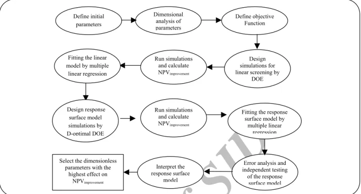
The complete layout of the project has been described schematically in Fig. 1. According to table 1, we started with selection of initial parameters. Then we changed input variables to dimensionless parameters to reduce their number and eliminate their dimensions (table 2). In other words, all the input variables were converted to dimensionless parameters by construction of the

dimensionless ratios. We aimed to examine the sensitivity of output function of the optimizer (NPV) in terms of the reservoir and fluid properties by constructing a response surface model. Therefore, the response function (NPVimprovement) was defined on the basis of NPV function

and dimensionless variables were considered as inputs of the response surface model. D-optimal technique was used to design the screening simulation runs. After running the simulations, multiple linear regression was considered to fit a linear model so that we could screen the major effects of dimensionless parameters on response function. Pareto charts were constructed to visualize the result of linear screening. After eliminating two initial dimensionless parameters (µo/µw, pres/pref) with

small effects on response function, final simulation runs were designed by using of three-level D-optimal technique. By running the simulations and recording the NPVimprovement for all the runs, full-quadratic response

surface model was constructed by using multiple linear regression. Pareto charts were plotted in order to depict the effects of linear interaction and squared terms of the response surface model. The next step was independent testing and error analysis of the model. It was done in order to examine the efficiency of the constructed response surface model.

Select the dimensionless parameters with the

highest effect on NPVimprovement

Error analysis and independent testing

of the response surface model Fitting the linear

model by multiple linear regression Run simulations and calculate NPVimprovement Define objective Function Dimensional analysis of parameters Define initial parameters Run simulations and calculate NPVimprovement

Fitting the response surface model by multiple linear regression Design simulations for linear screening by DOE Design response surface model simulations by D-optimal DOE Interpret the response surface model

Archive of SID

Table 1: Initial input parameters.

Initial variable Description

kxstreak Streak permeability in x-direction kystreak Streak permeability in y-direction kxmatrix Matrix permeability in y-direction kymatrix Matrix permeability in y-direction

µo Oil viscosity

µw Water viscosity

pr Reservoir pressure

qinj Water injection rate

Ls Length of streak

L Length of reservoir

Ws Width of streak

W Width of reservoir

Water cost Water production cost

Oil price Oil price

ϕ Porosity

Table 2: Initial dimensionless parameters.

Dimensionless group Description

ϕ Porosity

kmax/kmaxstreak Maximum permeability of matrix over _{maximum permeability of streak} Astreak Anisotropy of streak

Amatrix Anisotropy of matrix µo/µw Oil viscosity over water viscosity

Ws/W Width of streak over width of reservoir Ls/L Length of streak over length of reservoir pres/pref Reservoir pressure over reference _pressure Qinj/qref Water injection rate over reference water _{injection rate} (Water cost/Oil price) Water produced cost over oil price

CHARACTERISTICS OF THE OPTIMIZER

Reservoir model description

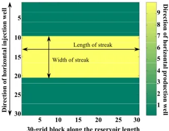
Water flooding optimizer assumes a heterogeneous, horizontal, two dimensional, two-phase (oil-water) reservoir with two horizontal smart wells, an injector and a producer, at opposite sides. The reservoir has no-flow boundaries at all sides. Each well is divided in segments with ICVs, allowing for individual inflow control of the segments [3]. Dimensions of the grid blocks are 30 m (length), 30m (width) and 10m (height). There are 30 grid blocks along the length and width of the reservoir. Therefore, the area of the reservoir is 900 m by 900 m. High permeable streaks can be defined in two-dimensionalreservoirmodelwith different lengths, widths and angle. The streaks cause early water breakthrough, and water flooding optimizer aims to maximize recovery or net present value over a given simulation time for heterogonous reservoirs that suffer from these high permeable streaks. Fig. 2 and Fig. 3 describe the heterogeneous, horizontal, two-dimensional reservoir. Injection and production wells are located at opposite sides of the reservoir and high permeable streaks are perpendicular to the direction of injection and production wells. Reservoir model includes two different parts: streak and matrix. They both have the same porosity, but different permeability in x and y-direction. Streaks with different lengths and widths can be defined for optimizer in order to monitor the effect of change of them on output function of the optimizer.

Methodology of the water flooding optimizer

- Water flooding optimizer has been developed on the basis of optimal control algorithm. Optimal control is a gradient-based optimization technique that is used to find the input variables that minimize or maximize a certain objective function. But maximizing or minimizing of the objective function is under limitation of different constraints of the system. Dynamic optimization involves the constraints of the system by using of Lagrange Multipliers [3]. Water flooding optimizer has considered two different options for reservoir constraints:

- Pressure constraint

- Rate constraint

We run all the designed simulations under the assumption of rate constraint.

Archive of SID

Fig. 2: Visualization of the dimensions of reservoir and a

selective high permeable streak. (Color bar shows the difference of permeability of matrix and high permeable streak).

DEFINING INPUT PARAMETERS AND OUTPUT RESPONSE FUNCTION

Initial input parameters

Table 1 introduces different input variables of the optimizer. Two-dimensional reservoir model assumes four different permeabilities (matrix permeability along x and direction, streak permeability along x and y-direction). Oil and water viscosity were the next input variables. Geometric dimensions of the high permeable streak and reservoir (i.e. length and width of the reservoir and streak) were the other input variables. Reservoir pressure, water injection rate, water production cost, oil price and reservoir porosity were the last selections for initial input parameters. Of course, there were some other variables such as capillary pressure (Pc), oil and water

compressibility (co , cw), and angle of streak, but their

small effects had already been confirmed by early simulation runs.

Output response function

NPV has been considered as objective function, which tends to be maximized by optimal control algorithm [3]. The objective function is equal to the NPV:

∑

− = ς = ς N1 0 m n ₍₁₎ where

Fig. 3: Top view of reservoir showing two-dimensional permeability of matrix and streak.

n Nprod 1 K t n k o o n k w w n _t ) 100 / b 1 ( ) q ( r ) q ( r yh x n ∆         + − ∆ ∆ = ς

∑

₌ (2)

The assumption is that the grid block volume ∆x∆yh and the cost/benefit coefficients rw, and ro are the same

for all well segments. The terms in the denominators of the sum terms introduce discounting. ς is the net present value function over a given time, b the annual interest rate which is expressed in %, tn _{the time expressed in}

whole years at time step n,qw produced water flow rate

and qo produced oil flow rate. Note that qoand qw have

negative sign and t is an exponent, where n is a superscript [3].

Generally, high permeable streaks cause early water breakthrough and water-flooding optimizer has been designed to maximize recovery in heterogeneous reservoirs. The optimizer improves the water flooding policy from different segments with iteration process. First of all, the optimizer performs water flooding without the use of optimizer algorithm (i.e. conventional water flooding). After that, the water injection policy proceeds on the basis of optimal control algorithm in order to maximize the net present of the water-flooding scenario.

Therefore, optimizer calculates net present value of the water flooding scenarios with and without using optimization algorithm. They were named as NPVoptimized

and NPVconventional, respectively. We defined NPVimprovement

9 8 7 6 5 4 3 2 1 5 10 15 20 25 30 5 10 15 20 25 30 30-grid block along the reservoir length

Direct ion of h oriz on tal in jectio n w ell Direct ion of h oriz on tal p rod uc tion well Length of streak Width of streak 5 10 15 20 25 30 30-grid block along the reservoir length

9 8 7 6 5 4 3 2 1 5 10 15 20 25 30

High permeable streak with 24-grid block length and 3-grid block width

30-grid block a

long the

width of the

reservo

Archive of SID

as response function in order to monitor the efficiency of the optimizer algorithm in different reservoir conditions:

al convention al convention optimized t improvemen _NPV NPV NPV NPV = − (3)

where NPVconventional is net present value without the use

of water flooding optimizer, NPVoptimized net present value

by means of optimizer algorithm and NPVimprovement the

fraction of net present value improvement.

Constant cumulative water injection

We considered one pore volume injection for all the simulation runs. In this case, we were sure that all the simulation runs reach to the breakthrough time and the reservoir is not depleted completely. We calculated simulation time for different runs by using the following formula:

Simulation time= (pore volume) /( injection rate) (4)

Design of experiments (DOEs)

Sometimes we want to know the sensitivity of output function of a system whit respect to the different input parameters. The system can be experimental set-up or simulation software. Therefore, we deliberately change one or more input parameters to observe the effects of the imposed perturbation on output function. One by one changing of the parameters is the traditional way of perturbing the input parameters. In this case, we have to change the input variables one by one and run the simulation or experimental set-up for all the parameter changes. This is not an efficient way, because it cannot consider the simultaneous effects of changes of different parameters and it is also very time- consuming. The statistical design of experiments (DOE) is a amuch more improved procedure for planning experiments so that data can be analyzed to give valid conclusions. DOE introduces different techniques in order to monitor the simultaneous changes of input parameters in a systematic way [6]. The technique is applied to choose a moderate number of simulation runs and analyze them to estimate the sensitivity of output function to various input parameters. In other words, well-chosen experimental designs can maximize the amount of information that can be obtained for a given amount of experimental design [6].

In order to construct a certain DOE design for simulator or experimental set-up, there was a need to define levels of extremes for each input variable. Two-level (i.e. minimum and maximum) and three-Two-level (i.e. minimum, intermediate, and maximum) designs are the most prevalent ones. Two-level designs cannot be used to predict the curvature shape of response surfaces. They only can construct linear response surfaces, whereas three-level designs can be used in order to construct nonlinear response surface models.

In linear screening of the initial dimensionless parameters, we defined two levels of extremes for each dimensionless parameter and we reached to the third intermediate level by averaging of maximum and minimum levels. Therefore, the three levels were used for construction of three-level D-optimal design. For example, porosity of the reservoir was one of the input dimensionless parameters. We considered 0.1 and 0.3 for minimum and maximum levels, respectively. They were used for linear screening. After screening out the dimensionless parameters, porosity was still one of the final dimensionless parameters. We need to have three levels for each final dimensionless parameter. Therefore, we obtained 0.2 for intermediate level of reservoir porosity by averaging of 0.1 and 0.3. Then the three levels were used for creating non-linear response surface model. Two levels of extremes were defined to make linear model and three levels of extremes were considered to create the nonlinear response surface model. Note that notations –1, 0, +1 describe minimum, intermediate and maximum levels of parameters, respectively. In general, designs are lists of combination of factors at which experiments or simulations are performed. In matrix notation, each row of the design matrix indicates a run, whereas each column contains the settings of each factor [6]. Table 3 and table 4 show the extreme levels of dimensionless parameters used for constructing the linear and nonlinear response surface models.

Full factorial designs are the simplest forms of DOE designs and the number of simulation runs for full factorial designs can be calculated by the following formula:

Number of full factorial runs= Lk ₍₅₎

Archive of SID

Table 3: Initial dimensionless parameters and their two-level

extremes for linear screening.

Dimensionless parameter Low extreme High extreme

φ 0.10 0.30

kmax/kmax streak 0.01 0.10

Astreak 0.01 1.00 Amatrix 0.01 1.00 µo /µw 0.10 10.00 Ws / W 0.03 0.33 Ls / L 0.80 1.00 Pres / pref 0.75 1.00 qinj / qref 0.60 1.00

(Water cost)/(Oil price) 0.05 0.20

Table 4: Levels of extremes for 3-level D-optimal design.

Dimensionless

parameter extremeLow

Intermediate level High extreme φ 0.1 0.2 0.3 kmax/kmaxtreak 0.01 0.055 0.1 Astreak 0.01 0.505 1 Amatrix 0.01 0.505 1 Ws/W 0.06 0.18 0.3 Ls/L 0.8 0.9 1 Qinj/qref 0.6 0.8 1 (Water cost) / (Oil price) 0.05 0.125 0.2

number of input parameters. The story of DOE design begins from full factorial design. Needless to say, full factorial designs include all the possible settings and are the most complete designs. But if we have much more input variables with three or more levels of extremes, the number of simulation runs will increase dramatically. Therefore, different techniques of DOE were invented in order to have moderate number of simulation runs with high amount of data information. Different techniques of DOE can be divided into two main groups:

- Classical experimental designs

- Optimal experimental design

The main difference between classical and optimal experimental designs is that classical designs are the ones created before the generation of computers, but optimal designs were developed after invention of computers. Therefore, classical designs are famous to first-generation of DOE designs and optimal experimental designs are called second-generation of DOE designs [7].

Optimal experimental design

Optimal experimental designs are called second-generation of DOE designs since they were developed after generation of computers. They are all based on mathematical optimality criterion. Hence, using of computer is inevitable for constructing optimal experi-mental designs. D-optimal DOE designs are the most important types of optimal experimental designs.

D-optimal design

The main idea of the D-optimal DOE design can be described by the following formula:

(Information) /(Simulation runs) = maximum. (6) In other words, D-optimal design helps to design simulation runs with the maximum amount of information and minimum number of simulation runs. D-optimal design is based on the following optimality criterion: Two column vectors X1 and X2 are orthogonal

if X1*X2=0 .The more dependent the vectors (columns) of

the design matrix, the closer to zero is the determinant of the correlation matrix for those vectors; the more independent the columns, the larger is the determinant of that matrix. Therefore, finding a design matrix that maximized the determinant D of the design matrix means finding a design where the factor effects are maximally independent of each other. This criterion for selecting a design is called D-optimality criterion [8].

We used two-level D-optimal design for constructing of linear matrix design. We generated 11 simulations runs for 10 initial dimensionless parameters. After that, three-level D-optimal design was used in order to create 50 simulation runs for eight dimensionless parameter. All the D-optimal matrix designs were generated by using of commands of statistics Toolbox of MATLAB software. Shape of the model (i.e. linear, interaction- linear,

Archive of SID

Fig. 4: DOE process for constructing of response surface models.

quadratic), number of desired runs and number of parameters were three essential input terms for construction of D-optimal matrix designs [9].

We used D-optimal designs for linear and non-linear modeling because they have been constructed on the basis of optimality criterion. Namely, they have maximum amount of information with minimum amounts of simulation runs. Therefore, they are always good candidates for making matrix designs. But the point is that D-optimal designs are created under the assumption of shape of response surface function. Therefore, D-optimal designs are always biased on the assumed shape of response surface model.

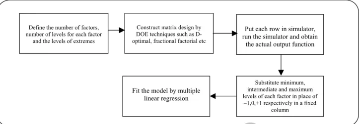
The complete procedure for construction of response surface models using design of experiments method has been described in Fig. 4.

RESPONSE SURFACE MODELS

Generally, the true relation between the different parameters of a system is really unknown. Therefore, finding an approximate solution as an empirical equation is a good way to predict the effect of input independent parameters on output dependent function. Response surface models are functions that are empirically fit to the observed data from results of experiments or simulation runs. They consider a polynomial empirical equation to predict the local shape of the response surface. That’s why they are named response surface models. Polynomial response surface models are most widely used so that we can find optimum or improved process settings [10].

Linear and quadratic response surface models are two

important kinds of polynomial response surface models. Besides, interaction terms can be added to empirical structure of response surface models. Therefore, there are different options in order to design the model equation. They are as follows:

- Constant term

- Linear term

- Interaction term

- Quadratic term

For instance, if we consider a system with two input variables (x1,x2), full quadratic response surface model

can be described by the following formula [11]:

2 2 22 2 1 11 2 1 1 2 2 1 1 0+β x +β x +β x x +β x +β x β = η (7)

As we see in the above formula, full quadratic response surface model, includes constant term (β0),

linear terms (β1x1+β2x2), interaction terms (β12x1x2) and

quadratic terms (β₁₁x₁2+β₂₂x2₂), where β0, β1, β2, β12,

β11, β12 are correspondent coefficients of different terms

of the equation and

η

is the model function. It is possible to construct the model function with different structures by the use of a combination of constant term, linear term(s), interaction term(s) and quadratic term(s) [12]. The following formulas describe some other options of response surface model with two input parameters (x1 , x2):

Simple linear model:

η=β0+β1x1+β2x2 (8)

Linear-interaction model:

Fit the model by multiple linear regression

Substitute minimum, intermediate and maximum levels of each factor in place of

–1,0,+1 respectively in a fixed column

Put each row in simulator, run the simulator and obtain

the actual output function Construct matrix design by

DOE techniques such as D-optimal, fractional factorial etc Define the number of factors,

number of levels for each factor and the levels of extremes

Archive of SID

2 1 12 2 2 1 1 o+β x +β x +β x x β = η (9) The notations used for the above formulas are the same as full quadratic response surface equation. Response surface models can be used as a proxy model for reservoir simulators in order to perform uncertainty analysis, parameters estimation and optimization.

Fitting the experimental design by multiple linear regression

We used multiple linear regression in order to fit the linear and non-linear response surface models. Multiple linear regression is a statistical technique that allows us to predict one dependent variable with respect to several independent variables [13].

Multiple linear regression is multidimensional linear regression on the basis of Least square method. Least square method assumes that the best curve-fit of data is the curve that has the minimal sum of the deviations squared (least square error) from a given series of data. Suppose that the data points are:

) y , x ,..., y , x ( ), y , x ( 1 1 2 2 n n (10)

Where x is independent variable and y is the dependent variable. The fitting curve f(x) has the deviation (error) d from each data point. According to the method of least squares, the best fitting curve should satisfy the following formula:

[

y f(x )

]

Minimum d n 1 i 2 i i n 1 i 2 i =

∑

− =

∑

= = (11)

Generally, the purpose of multiple linear regression is to find a relationship between a group of input parameters (the columns of x) and a response, y. This relationship is useful for understanding which parameters have the greatest effect, knowing the direction of the effect (i.e., increasing x increases/decreases y) and using the model to predict future values of the response when only the predictors are currently known [13]. The linear model can be described by the following formula:

ε + β =X

y (12) where y is an n-by-1 vector of observations, X an n-by-p matrix of repressors, β a p-by-1 vector of parameters and

ε an n-by-1 vector of random disturbances. The solution to the problem is a vector, b, which estimates the

unknown vector of parameters, β. The least squares solution is: y X X) (X βˆ b_{= =} T −1 T ₍₁₁₎

Generally, the purpose of multiple linear regression is to find a relationship between a group of input parameters (the columns of x) and a response, y. This relationship is useful for understanding which parameters have the greatest effect, knowing the direction of the effect (i.e., increasing x increases/decreases y) and using the model to predict future values of the response when only the predictors are currently known [13]. The linear model can be described by the following formula:

ε + β =X

y (12) where y is an n-by-1 vector of observations, X an n-by-p matrix of repressors, β a p-by-1 vector of parameters and

ε an n-by-1 vector of random disturbances. The solution to the problem is a vector, b, which estimates the unknown vector of parameters, β. The least squares solution is: y X ) X X ( ˆ b=β= T −1 T (13)

We used multiple linear regression in order to solve the combination of simulation design equation. All the linear and nonlinear models were fitted by using of commands of Statistics Toolbox of MATLAB software.

Linear screening of the parameters

The primary purpose of the linear screening is to select or screen out the few important main effects from the many less important effects. Linear screening designs are also named main effects designs. The methodology of linear screening applies solving a linear program with the regression function, estimated through linear regression analysis, as the objective function. Linear screening assumes that input parameters are completely inde-pendent of each other. Therefore, it is not a real response surface model. It is usually done to screen the major effects of the initial input parameters. According to the results of linear screening, unnecessary initial parameters with the least degrees of effects will be eliminated. Therefore, final nonlinear response surface model is constructed on the basis of the most important input parameters. We selected 10 different dimensionless

Archive of SID

Fig. 5: Pareto chart showing linear model coefficients.

groups and considered a simple linear model for linear screening:

∑

= β + β = 10 1 i i i 0 t improvemen x V Pˆ N (14)

where xi and βi represent the dimensionless groups and

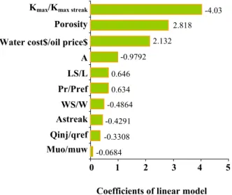
their correspondent coefficients, respectively. We considered two extremes for each dimensionless group and substituted them in a two-level D-optimal design and considered a simple linear model (for 10 initial dimensionless parameters) in order to fit 11 simulation runs of screening part by multiple linear regression. Finally we derived the linear model coefficients by using multiple linear regression technique. Pareto graphs were constructed to visualize the results of screening part .See Fig. 5 and Fig. 6.

It should be reminded that Pareto Chart is a special form of a bar graph and is widely used to display the relative importance of problems or conditions. Pareto charts graphically order the effects of factors with respect to the response function so that the most important effects (main effects) can come to the surface. In general, a Pareto chart is used for focusing on critical issues by ordering them in terms of importance and frequency, prioritizing problems and analyzing problems by different groupings of data.

Constructionof response surface model

Generally, the structure of the relationship between the response and the independent variables is unknown.

Fig. 6: Pareto chart showing normalized effects of dimensionless groups in linear model.

The most important step in the construction of response surface model is to find a suitable approximation to the real relationship. The most common forms of response surface models are low-order polynomials (first or second-order). First-order models are widely used for screening of the initial input parameters and second-order response surface models are the most common forms of nonlinear response surface models. They are also famous to the full-quadratic response surface models. They include linear, square and interaction terms. The second-order model, in general form, is given as:

∑∑

∑

β + β + β = η 2 _{ij i j} j jj 0 x x x (15)

where η is full-quadratic response surface model, βo the

constant term,

∑

β_jx_j linear terms,

∑

β 2 j

jjx square

terms and

∑∑

β_ijx_ix_j interaction terms. Note that

β0, βj, βjj and βij are correspondent coefficients of

different terms.

The major effects of initial dimensionless parameters had already been monitored by linear screening. Referring to the linear screening results, we eliminated two dimensionless parameters (µo/µw, pres/pref) with small

effects on output response function and selected eight final dimensionless parameters. We constructed a full-quadratic response surface model with eight dimen-sionless parameters. A full-quadratic response surface model with eight variables includes one constant term,

Coefficients of linear model 0 1 2 3 4 5 Kmax/Kmax streak

Porosity Water cost$/oil price$ A LS/L Pr/Pref WS/W Astreak Qinj/qref Muo/muw -4.03 2.818 2.132 -0.9792 0.646 0.634 -0.4864 -0.4291 -0.3308 -0.0684 0 10 20 30 40 50 Normalized effects of dimensionless groups Kmax/Kmax streak

Porosity Water cost$/oil price$ A LS/L Pr/Pref WS/W Astreak Qinj/qref Muo/muw 32.10 % 22.44 % 16.99 % 7.80 % 5.15 % 5.05 % 3.87 % 3.42 % 2.63 % 0.54 %

Archive of SID

eight linear terms (main effects of each input parameter), eight square terms (square terms of each input parameter) and 28 interaction terms (all the bilateral effects of the input parameters). Totally constructed full-quadratic response surface model included 45 terms.

We designed 50 simulation runs by using three-level D-optimal technique of DOEs for eight parameters. Afterrunning the simulations and calculating NPVimprovement for all the runs, we obtained the 50 by 1

solution matrix (y). Then we completed 50 by 45 information matrix (X) by multiplying and squaring the correspondent pre-designed main effects. Using multiple linear regression, we obtained 45 by 1 coefficient matrix (β) of full-quadratic response surface model. Finally Pareto charts were constructed in order to visualize the effects of 45 terms of full-quadratic response surface model. See Fig. 7.

Independent testing of response surface model by perturbation of DOE design

Response surface models are always biased to the levels of designs. Namely, they are constructed by the extremes of the input parameters. On the other hand, the structure of the relationship between the response function and input parameters is unknown and construction of response surface models is done on the basis of finding a suitable approximation to the actual relationship. Hence, response models are always biased on levels of the input parameters and the pre-assumed structure of the model. Therefore, we perturbated the DOE design by generating ten new simulation designs to see the efficiency of the model for predicting the simulation runs. The perturbing design was generated by defining new extremes on the basis of linear model assumption. It was done in order to impose changes to the main DOE design to see the effects of the perturbation on output function of the model. We defined the perturbing runs by two-level D-optimal DOE technique and calculated actual NPVimprovement for each run. On the other

hand, we calculated NPVimprovement by using of the

non-linear surface response model. Comparison of the actual and calculated NPV was done in order to examine the efficiency of the constructed response surface model in predicting the output response function, Fig. 8 depicts the ability of the model for predicting the recovery improvement scenarios. Error analysis was done in order

Fig. 7: Pareto chart showing the normalized effects of nonlinear response surface model.

Fig. 8: Scattered plot showing five points of independent testing.

to examine the efficiency of the proposed response surface model. Table 5 and table 6 show the results of error analysis in detail.

RESULTS AND DISCUSSION

Linear screening

Linear screening always is done to detect the input parameters with the major degrees of importance.

0.00 0.01 0.02 0.03 0.04 0.05 0.06 NPV actual 0.10 0.09 0.08 0.07 0.06 0.05 0.04 0.03 0.02 0.01 0.00 NPV model G Cl I2 G2 CG BI CF A CH B BC C2 BG F2 B2 BH I BF FH F FG DI H EI GI EG D DG E H2 BD GH CD C DH EH EF DF HI CE D2 DE E2 FI BE 0.00 2.00 4.00 6.00 8.00 10.00 12.00 14.00 Percentage effect 11.99 % 8.92 % 8.74 % 7.16 % 6.81 % 6.65 % 6.16 % 5.97 % 5.41 % 2.84 % 2.71 % 2.31 % 2.10 % 2.10 % 1.69 % 1.45 % 1.35 % 1.39 % 1.34 % 1.25 % 1.19 % 1.15 % 1.10 % 1.05 % 0.66 % 0.65 % 0.64 % 0.55 % 0.52 % 0.51 % 0.50 % 0.47 % 0.45 % 0.45 % 0.36 0.29 % 0.22 % 0.20 % 0.18 % 0.15 % 0.11 % 0.09 % 0.07 % 0.06 % 0.045 % A Constant term B Porosity C Kmax / Kmaxstreak D Astreak E A F Ws/W G Ls/L H qinjection/qref I Water cost ($)/Oil price($)

Archive of SID

Table5: selective independent testing of the model.

Runs NPV actual NPV model

1 0.021 0.046

2 0.0485 0.089

3 0.0122 0.0157

4 0.0027 0.0046

5 0.0232 0.0339

Table 6: The results of error analysis.

Mean absolute error 0.01632

Mean NPV actual 0.02152

Mean abs error/Mean NPV

actual 0.75836

Namely, linear screening is a rough estimate for monitoring the sensitivity of the output response function with respect to the different input parameters. It doesn’t cover interaction and second order terms.

Therefore, linear model is not a real response surface model and is unable to pinpoint the effects of different parameters exactly. However, referring to the Pareto charts that show the screening results of initial dimensionless parameters (Fig. 5 and Fig. 6), kmax/kmax

has the highest effect on output response function. On the other hand, µo/µw has the least importance and the effects

of the other dimensionless parameters are between these to extreme effects. Geometric factors (Ws/W, Ls/L) with

moderate effects are in the middle of the order of the Pareto chart.

Full quadratic response surface model

According to the non-linear response surface model (Fig. 7) main effect G (length of streak over length of reservoir) has the maximum effect on output response function. Square term G2 _{and interaction term CG also}

have high effects on response function. Therefore, it is safe to say that length of streak over length of reservoir has the highest effect on output function. Interaction term Cl and square term I2 _{are the second and third terms in}

Pareto chart ranking. As a result, financial dimensionless group I (water cost over oil price) is the second important dimensionless group. Referring to the position of interaction terms Cl, CG and CF, one can find out that C(kmax/kmaxstreak)) is the third important dimensionless

parameter. The other terms have the lower degrees of effect. It can be concluded that interaction and square terms have important effects on response surface function. Therefore, they affect the ranking of the different terms and this is the main reason for the difference between the results of linear screening and non-linear surface response model.

Length of streak and variation of matrix and high permeable streak permeability both intensify early water breakthrough. Surprisingly, the effect of porosity on NPVimprovement is quite considerable, whereas we expected

that porosity couldn’t play an important role on NPVimprovement.However, the model should be improved

(i.e. by increasing simulation runs), in order to judge on the importance of the other terms at the bottom of the Pareto graph.

Independent testing of the response surface model A number of 10 independent runs were designed in order to examine the fitting efficiency of the model. Table 6 shows the results of independent testing of the model. As we see, response surface model has predicted simulation runs with an acceptable amount of error. Fig. 8 depicts the scattered graph of independent testing results. It shows that response surface model is successful to predict these simulation runs.

It can be imagined that there is a parabolic trend between the number of simulation runs and fitting efficiency of the response surface model and that by increasing simulation runs, fitting efficiency of the model will increase dramatically, but after that, the slope will be smoothed gradually. However, increasing simulation runs is highly recommended to complete the response surface model as a fast proxy model.

Recommendations

- Increase the number of simulation runs to complete the response surface model.

- Try other options for alternative response surface models, i.e. cubic or logarithmic models.

CONCLUSIONS

1- The scope to improve water flooding in a two-dimensional square reservoir produced with two rows of injection and production wells and containing a single heterogeneous streak can be described with the aid of 10 dimensionless parameters.

Archive of SID

2- Initial screening using a linear response model based on 11 water-flooding simulations indicated that only 8 dimensionless parameters are statistically significant.

3- More complicated response surface models can be easily obtained with the aid of design-of-experiments techniques. In particular, we developed a full quadratic response surface model based on 50 simulations.

4- These simulation runs show an average scope of improvement of 23.7 %.

5- An independent verification of the quality of the full quadratic response surface model, using another 10 simulations, reveals that some more simulations is needed to obtain a more reliable response surface model.

6- Based on the present model we conclude that the parameters Ls/L (relative streak length), kmax/kmaxstreak

(relative streak permeability) and the ratio of water cost and oil price have the largest effect on the scope to improve water flooding. The scope for improvement increases with larger relative streak length, larger permeability contrast, and relatively high water costs.

Nomenclatures

NPV Net present value NPVimprovement Net present value improvement

NPVconventional Net present value without optimizer

NPVoptimized Net present value with optimizer

n Time step

N Final time step

r Price per unit volume ,($/m3₎

∆t Time interval, (s)

qo Oil flow rate, (m3/s)

qw Water flow rate, (m3/s)

b Annual interest rate

h Reservoir height, (m) kmaxstreak Maximum permeability of streak, (m2)

kmax Maximum permeability of matrix, (m2)

L Length of reservoir, (m)

Ls Length of streak, (m)

Ws Width of reservoir, (m)

W Width of streak, (m)

A Matrix anisotropy

Astreak Streak anisotropy

ϕ Porosity

µo Oil viscosity, (Pa.s)

µw Water viscosity, (Pa.s)

pres Reservoir pressure, (Pa)

pref Reference pressure, (Pa)

qinj Injection rate, (m3/s)

qref Reference injection rate, (m3/s)

kymatrix Matrix permeability in y direction, (m2)

kystreak Streak permeability in y direction, (m2)

kystreak Streak permeability in y direction, (m2)

kxmatrix Matrix permeability in x direction, (m2)

RSM Response surface model co Oil compressibility, (1/Pa)

cw Water compressibility, (1/Pa)

pc Capillary pressure, (Pa)

ICV Internal Control Valve

Received : 14th _{September 2005 ; Accepted : 17}th _{August 2006}

REFERENCES

[1] Asheim, H., Maximization of Water Sweep Effi-ciency by Controlling Production and Injection Rates, paper SPE 18365,(1991).

[2] Brouwer, D.,R., Jansen, J.,D., van der Starre, S., and Van Kruijsdijk, C.P.J.W., Recovery Increase through Water Flooding using Smart Well Technology, paper SPE 68979, (2000).

[3] Brouwer, D., R., and Jansen, J.D., Dynamic Optimization of Water Flooding with Smart Wells Using Optimal Control, paper SPE 78278, (2001). [4] Sudaryanto, B., and Yortsos, Y., C., Optimization of

Fluid Front Dynamics in Porous Media Using Rate Control,. I. Equal Mobility Fluids, Phys. of Fluids,

12 (7), 1656, (2000).

[5] Yeten,B.,Durlofsky, L.J. and Aziz, K., Optimization of Smart Well Control, paper SPE 79031, (2001). [6] Box, G.E.P., Hunter, W.G. and Hunter, J.S.,

“Statistics for Experimenters”, John Wiley & Sons, (1978).

[7] Friedmann, F., Chawathe, A. and Larue, D., Assessing Uncertainty in Channelized Reservoirs usingExperimentalDesigns,paperSPE71622,(2000). [8] Atkinson, A. C. and Donev A. N., Optimum

Experi-mental Designs, Oxford University Press, Oxford, UK, (1992).

[9] Cook, R.D. and Nachtsheim, C.J., A Comparison of Algorithms for Constructing exact D-Optimal Designs, Technometrics, 22 (3), August (1980). [10] Narayanan, K., Applications for Response Surfaces

Archive of SID

in Reservoir Engineering, MS Thesis, University of Texas, Austin, (1999).

[11] Draper, N. R. and Lin, D. K. J., Small Response-Surface Designs, Technometrics, 32,187 (1990). [12] Box, G.E.P. and Draper, N.R., “Empirical

Model-Building and Response Surface”, John Wiley and Sons, (1987).

[13] Montgomery, D. C. and Peck, E. A., “Introduction to Linear Regression Analysis”, John Wiley and Sons, (1982).