Dual Averaging for Distributed Optimization:
Convergence Analysis and Network Scaling
John C. Duchi, Alekh Agarwal, and Martin J. Wainwright
, Senior Member, IEEE
Abstract—The goal of decentralized optimization over a net-work is to optimize a global objective formed by a sum of local (possibly nonsmooth) convex functions using only local computa-tion and communicacomputa-tion. It arises in various applicacomputa-tion domains, including distributed tracking and localization, multi-agent coor-dination, estimation in sensor networks, and large-scale machine learning. We develop and analyze distributed algorithms based on dual subgradient averaging, and we provide sharp bounds on their convergence rates as a function of the network size and topology. Our analysis allows us to clearly separate the convergence of the optimization algorithm itself and the effects of communication dependent on the network structure. We show that the number of iterations required by our algorithm scales inversely in the spectral gap of the network, and confirm this prediction’s sharpness both by theoretical lower bounds and simulations for various networks. Our approach includes the cases of deterministic optimization and communication, as well as problems with stochastic optimization and/or communication.
Index Terms—Convex optimization, distributed control, dis-tributed multi-agent system, disdis-tributed optimization, subgradient algorithms.
I. INTRODUCTION
T
HE focus of this paper is the development and analysis of distributed algorithms for solving convex optimization problems that are defined over networks. Network-structured optimization problems arise in a variety of domains within the information sciences and engineering. For instance, problems such as multi-agent coordination, distributed tracking and lo-calization, estimation problems in sensor networks and packet routing are all naturally cast as distributed convex minimization [1]–[4]. Common to these problems is the necessity for com-pletely decentralized computation that is locally light—to avoid overburdening small sensors or flooding busy networks—and robust to periodic link or node failures. As a second example,Manuscript received May 17, 2010; revised November 11, 2010 and April 10, 2011; accepted June 17, 2011. Date of publication June 30, 2011; date of current version February 29, 2012. This work was supported in part by NSF-CAREER-0545862 and AFOSR-09NL184. The work of J. C. Duchi was supported by a National Defense Science and Engineering Graduate Fellowship (NDSEG). The work of A. Agarwal was supported by a Microsoft Research Fellowship. A preliminary version of this paper appeared in the Proceedings of the 24th Neural Information Processing Systems conference, Vancouver, BC, Canada, in 2010. Recommended by Associate Editor S. Mascolo.
J. C. Duchi and A. Agarwal are with the Department of Electrical Engineering and Computer Sciences, University of California at Berkeley, Berkeley, CA 94720 USA (e-mail: [email protected]; [email protected]).
M. J. Wainwright is with the Department of Electrical Engineering and Com-puter Sciences, University of California at Berkeley, Berkeley, CA 94720 USA, and also with the Department of Statistics, University of California at Berkeley, Berkeley, CA 94720 USA (e-mail: [email protected]).
Color versions of one or more of thefigures in this paper are available online at http://ieeexplore.ieee.org.
Digital Object Identifier 10.1109/TAC.2011.2161027
data sets too large to be processed quickly by any single pro-cessor present related challenges. A canonical instance from sta-tistical machine learning is the problem of minimizing a loss function averaged over a large dataset (e.g., support vector ma-chines [5]). With terabytes of data, it is desirable to assign sub-sets of the data to different processors, and the processors must communicate tofind parameters minimizing the loss over the entire dataset. However, the communication should be efficient enough that network latencies do not offset computational gains. Distributed computation has a long history in optimization, and the 1980s saw significant interest in distributed detection, consensus, and minimization. Earlier seminal work [1], [6], [7] analyzed algorithms for minimization of a smooth function known to several agents while distributing processing of components of the parameter vector . More recently, a few researchers have shifted focus to problems in which each processor locally has its own convex (potentially non-differen-tiable) objective function [8]–[11].
Our paper makes two main contributions to this area. Thefirst contribution is to provide a new simple subgradient algorithm for distributed constrained optimization of a convex function; we refer to it as a dual averaging subgradient method, since it is based on maintaining and forming weighted averages of subgradients throughout the network. This approach is essen-tially different from previously developed methods [8]–[10], and these differences facilitate our analysis of network scaling issues, meaning how convergence rates depend on network size and topology. Indeed, the second main contribution of this paper is a careful analysis that demonstrates a close link between con-vergence of the algorithm and the underlying spectral properties of the network.
By comparison to previous work, our convergence results and proofs are different, and our characterization of network scaling terms is often much stronger. As detailed comparison with past work requires presentation of several of our results, we give only a brief overview of related work here, deferring detailed discussion to Section IV. The sharpest results given previously for distributed projected gradient descent are dis-cussed in the papers [10] and [12] where it is shown that if the number of time steps is known a priori and the stepsize is chosen optimally, an -optimal solution to the optimization problem can be reached in time. Since this bound is essentially independent of network topology, it does not capture the intuition that distributed algorithms should converge much faster on “well-connected” networks—expander graphs being a prime example—than on poorly connected networks (e.g., chains, trees or single cycles). Johanssonet al.[11] analyze a low communication peer-to-peer protocol that attains rates de-pendent on network structure; however, in their algorithm only
one agent has a current parameter value, while all agents in our algorithm maintain good estimates of the optimum at all times. This is important in online, streaming, and control prob-lems where agents are expected to act in real time. In additional comparison to previous work, our development yields network scaling terms that are often substantially sharper; specifically, our convergence rate scales inversely in the spectral gap of the network. This allows us to build on known results to show that our algorithm obtains an -optimal solution in itera-tions for a single cycle or path, iterations for a two-di-mensional grid, and iterations for a bounded degree expander graph. We also show that the network deviation terms we derive are tight for our algorithm. Moreover, results on a simulated system identification task using robust linear regres-sion show excellent agreement with our theoretical predictions. Our analysis covers several settings for distributed minimiza-tion. We begin by studying fixed communication protocols, which are of interest in areas such as cluster computing or sensor networks with a fixed hardware-dependent protocol. We also investigate randomized communication protocols and randomized network failures, which are essential to handle gracefully in wireless sensor networks and large clusters with potential node failures. Randomized communication provides an interesting tradeoff between communication savings and convergence rates. In this setting, we obtain sharper results than previous work by studying the spectral properties of the expected transition matrix of a random walk on the underlying graph. We also present a relatively straightforward extension of our analysis for problems with stochastic gradient information. The remainder of this paper is organized as follows. Section II is devoted to a formal statement of the problem and descrip-tion of the dual averaging algorithm, whereas Secdescrip-tion III states the main results and consequences of our paper, which we com-plement in Section IV with a comparison to previous work. In Section V, we state and prove basic convergence results on the dual averaging algorithm, which we then exploit in Section VI to derive concrete results that depend on the spectral gap of the net-work. Sections VII and VIII treat extensions with noise, in par-ticular algorithms with random communication and stochastic gradients respectively. In Section IX, we present the results of simulations that confirm the sharpness of our analysis.
II. PROBLEMSETUP ANDALGORITHM
In this section, we provide a formal statement of the distributed minimization problem and a description of the distributed dual averaging algorithm.
A. Distributed Minimization
We consider an optimization problem based on functions that are distributed over a network. More specifically, let be an undirected graph over the vertex set with edge set . Associated with each is convex function , and our overarching goal is to solve the optimization problem
subject to (1)
where is a closed convex set. Each function is convex and hence sub-differentiable, but need not be smooth. We assume without loss of generality that , since we can simply trans-late . Each node is associated with a separate agent, and each agent maintains its own parameter vector . The graph imposes communication constraints on the agents: in particular, agent has local access to only the objective func-tion and can communicate directly only with its immediate
neighbors .
Problems of this nature arise in a variety of application do-mains. A concrete motivating example is the machine learning problemfirst described in Section I. In this case, the set is the parameter space of the statistician or learner. Each function is the empirical loss over the subset of data assigned to processor
, and assuming that each subset is of equal size (or that the are normalized suitably), the function is the average loss over the entire dataset. If we use cluster computing as our computa-tional model, then each processor is a node in the cluster, and contains edges between processors that are directly connected with small latencies.
B. Standard Dual Averaging
Our algorithm is based on Nesterov’s recent dual averaging algorithm [13], [14], designed for minimization of (potentially nonsmooth) convex functions subject to the constraint . We begin by describing the standard version of the algorithm and then discuss the extensions for the distributed setting of in-terest in this paper. The dual averaging scheme is based on a
proximal function assumed to be -strongly convex with respect to some norm , that is
for
In addition, we assume that over and that ; these are standard assumptions made without loss of generality. Examples of such proximal and norm pairs include:
• The quadratic , which is the canonical proximal function. Clearly , and
is strongly convex with respect to the -norm for . • The entropic function , which is strongly convex with respect to the -norm for in the probability simplex, .
We assume that each function is -Lipschitzwith respect to the same norm —that is
for (2) Many cost functions satisfy this type of Lipschitz condition. For instance, condition (2) holds for any convex function on a compact domain, or for a polyhedral function on an arbitrary domain [15]. The bound (2) implies that for any and any subgradient , we have , where de-notes thedual normto , defined by . The dual averaging algorithm generates a sequence of iter-ates contained within according to the following steps. At time step of the algorithm, it receives a subgradient , and then performs the updates
where is a non-increasing sequence of positive step-sizes, and
(4) is a type of projection. The intuition underlying this algorithm is as follows: given the current iterate , the next it-erate to chosen to minimize an averagedfirst-order approximation to the function , while the proximal function and stepsize enforce that the iterates do not oscillate wildly. The algorithm is similar to the “follow the perturbed leader” algorithms developed for online optimization [16], though this specific algorithm seems to be due to Nesterov [13]. In Section V, we show that a simple analysis of the con-vergence of the above procedure allows us to relate it to the dis-tributed algorithm we describe.
C. Distributed Dual Averaging
We now consider an appropriate and novel extension of dual averaging to the distributed setting. At each iteration , the algorithm maintains pairs of vectors , with the pair associated with node . At iteration , each node computes an element in the subdifferential of the local function and receives information about the parameters associated with nodes in its neighborhood . Its update of the current estimated solution is based on a convex combination of these parameters. To model this weighting process, let be a matrix of non-negative weights that respects the structure of the graph , meaning that for , only if . We assume that is a doubly stochastic matrix, so that
for all and
for all
Using this notation, given the non-increasing sequence of positive stepsizes, each node performs the updates
and (5a) (5b) where the projection was defined previously (4). In words, node computes the new dual parameter from a weighted average of its own subgradient and the param-eters in its neighborhood , and then computes the next local iterate by a projection defined by the proximal function and stepsize .
In the sequel, we show convergence of the local sequence to the optimum of (1) via therunning local average
(6)
Note that this quantity is locally defined at node and can be computed in a distributed manner.
III. MAINRESULTS ANDCONSEQUENCES
We will now state the main results of this paper and illustrate some of their consequences. We give the proofs and a deeper investigation of related corollaries in the sections that follow.
A. Convergence of Distributed Dual Averaging
We start with a result on the convergence of the distributed dual averaging algorithm that provides a decomposition of the error into an optimization term and the cost associated with net-work communication. In order to state this theorem, we define the averaged dual variable , and we recall the definition (6) of the local average .
Theorem 1 (Basic Convergence): Let the sequences and be generated by the updates (5a), (5b) with step size sequence , where is strongly convex with respect to the norm with dual norm . For any and for each node , we have
(7) where
and (8)
Theorem 1 guarantees that after steps of the algorithm, every node has access to a locally defined quantity such that the difference is upper bounded by a sum of four terms. The two terms in the OPTportion of the
upper bound (7) are optimization error terms common to sub-gradient algorithms. The third and fourth (NET) are penalties
incurred due to having different estimates at different nodes in the network, and they measure the deviation of each node’s es-timate of the average gradient from the true average gradient.1
Thus, Theorem 1 ensures that as long the bound on the deviation is tight enough, for appropriately chosen (say ), the error of is small uniformly across all nodes, and asymptotically approaches zero. See Theorem 2 for a precise statement of rates.
B. Convergence Rates and Network Topology
We now turn to investigation of the effects of network topology on convergence rates. In this section,2 we assume
that the network topology is static, and that communication occurs via a fixed doubly stochastic weight matrix at every round. Since is doubly stochastic, it has largest singular value (see [17, Ch. 8]). The following result shows that the convergence rate of the distributed dual averaging algorithm is controlled by thespectral gap
1The fact that the term appears an extra time is insignificant,
as we will bound the difference uniformly for all .
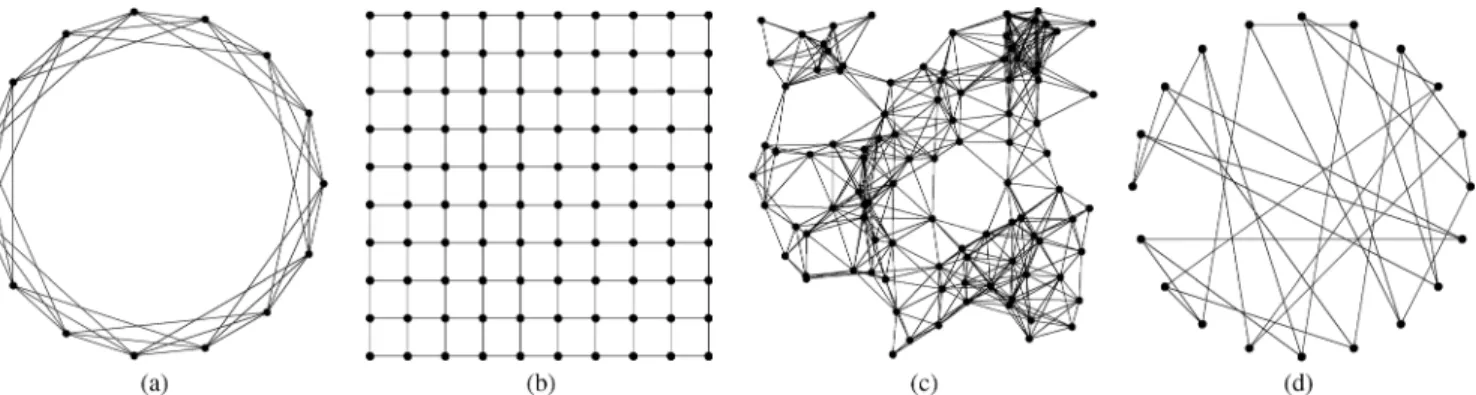
Fig. 1. Illustration of some graph classes of interest in distributed protocols. (a) A 3-connected cycle. (b) Two-dimensional grid with 1-connectivity, and non-toroidal boundary conditions. (c) A random geometric graph. (d) A random 3-regular expander graph.
of the matrix , where is the second largest singular value of .
Theorem 2 (Rates Based on Spectral Gap): Under the conditions and notation of Theorem 1, suppose more-over that . With step size choice
for all
This theorem establishes a tight connection between the con-vergence rate of distributed subgradient methods and the spec-tral properties of the underlying network. The inverse depen-dence on the spectral gap is quite natural, since it is well-known to determine the rates of mixing in random walks on graphs [18], and the propagation of information in our al-gorithm is integrally tied to the random walk on the underlying graph with transition probabilities specified by .
Using Theorem 2, one can derive explicit convergence rates for several classes of interesting networks, and Fig. 1 illustrates four graph topologies of interest. As afirst example, the -con-nected cycle in panel (a) is formed by placing nodes on a circle and connecting each node to its neighbors on the right and left. For small , the cycle graph is poorly connected, and our analysis will show that this leads to slower convergence rates than other graphs with better connectivity. The grid graph in two dimensions is obtained by connecting nodes to their nearest neighbors in axis-aligned directions. For instance, panel (b) shows an example of a degree 4 grid graph in two-dimen-sions. The cycle and grid are possible models for clustered com-puting as well as sensor networks.
In panel (c), we show a random geometric graph, constructed by placing nodes uniformly at random in and connecting any two nodes separated by a distance less than some radius . These graphs are used to model the connectivity patterns of devices, such as wireless sensor motes, that can communicate with all nodes in somefixed radius ball, and have been studied extensively (e.g., [19], [20]). There are natural generalizations to dimensions as well as to cases in which the spatial positions are drawn non-uniformly.
Finally, panel (d) shows an instance of a bounded degree ex-pander, which belongs to a special class of sparse graphs that have very good mixing properties [21]. Expanders are an at-tractive option for the network topology in distributed computa-tion since they are known to have large spectral gaps. For many
random graph models, a typical sample is an expander with high probability; examples include random bipartite [22] and random degree-regular graphs [23]. In addition, there are several deter-ministic constructions of degree regular expanders (see Chung [21, Sec, 6.3]). The deterministic constructions are of interest because they can be used to design a network, while the random constructions are often much simpler.
In order to state explicit convergence rates, we need to specify a particular choice of the matrix that respects the graph struc-ture. Although many such choices are possible, here we focus on the graph Laplacian [21]. First, we let be the symmetric adjacency matrix of the undirected graph , satis-fying when and otherwise. For each node , we let de-note the degree of node , and we define the diagonal matrix . We assume that the graph is connected, so that for all , and hence is invertible. With this no-tation, thenormalized graph Laplacianis
The graph Laplacian is symmetric, positive semidef-inite, and satisfies , where is the all ones vector. When the graph is degree-regular ( for ), the stan-dard random walk with self loops on given by the matrix
is doubly stochastic and valid for our theory. For non-regular graphs, we make a minor modification in order to obtain a doubly stochastic matrix: let de-note ’s maximum degree and define
(9) This matrix is symmetric by construction and it is also doubly stochastic. Note that if the graph is -regular, then is the standard choice above. Plugging into Theorem 2 imme-diately relates the convergence of distributed dual averaging to the spectral properties of the graph Laplacian; in particular, we have
(10) where is the second smallest eigenvalue of . The next result summarizes our conclusions for the choice of stochastic matrix (9) via (10) for different network topologies.
Corollary 1: Under the conditions of Theorem 2, we have the following convergence rates:
1) For -connected paths and cycles
2) For -connected grids,
3) For random geometric graphs with connectivity radius for any , with high-proba-bility
4) For expanders with bounded ratio of minimum to max-imum node degree
Note that up to logarithmic factors, the optimization term in the convergence rate is always of the order , while the remaining terms vary depending on the network. In order to understand scaling issues as a function of network size and topology, it can be useful to restate convergence rates in terms of the number of iterations required to achieve error for a network type with nodes. In particular, Corollary 1 implies the following scalings (to logarithmic factors):
• for the single cycle graph, ; • for the two-dimensional grid, ; • for a bounded degree expander, . In general, Theorem 2 implies that at most
(11) iterations are required to achieve an -accurate solution when using communication matrix . A detailed comparison of these results with the previous work is provided in Section IV.
It is interesting to ask whether the upper bound (11) from our analysis is actually a sharp result, meaning that it cannot be im-proved (up to constant factors). On one hand, it is known that (even for centralized optimization algorithms), any subgradient method requires at least iterations to achieve -accu-racy [24], so the term is unavoidable. The next proposition addresses the complementary issue, namely whether the inverse spectral gap term is unavoidable for the dual averaging algo-rithm, by establishing a lower bound on the number of iterations in terms of graph topology:
Proposition 1: Consider the dual averaging algorithm (5a) and (5b) with quadratic proximal function and communication matrix . For any graph with nodes, the number of iterations required to achieve afixed accuracy is lower bounded as
The proof of this result, given in Section VI-C, involves con-structing a “hard” optimization problem and lower bounding the number of iterations required for our algorithm to solve it. In conjunction with Corollary 1 and the bound (11), Proposition 1 implies that our predicted network scaling is sharp. Indeed, in Section IX, we show that the theoretical scalings from Corol-lary 1—namely, quadratic, linear, and constant in network size
—are well-matched in simulations.
C. Extensions to Stochastic Communication Links
Our results also extend to the case when the communication matrix is time-varying and random—that is, the matrix is potentially different for each and randomly chosen (but still obeys the constraints imposed by ). Such stochastic com-munication is of interest for a variety of reasons. If there is an un-derlying dense network topology, we might want to avoid municating along every edge at each round to decrease com-munication and network congestion. For instance, the use of a gossip protocol [25], in which one edge in the network is ran-domly chosen to communicate at each iteration, allows a more refined tradeoff between communication cost and number of it-erations. Communication in real networks also incurs errors due to congestion or hardware failures, and we can model such er-rors by a stochastic process.
The following theorem provides a convergence result for the case of time-varying random communication matrices. In par-ticular, it applies to sequences and gener-ated by the dual averaging algorithm with updates (5a) and (5b) with step size sequence , but in which is replaced with .
Theorem 3 (Stochastic Communication): Let
be an independent and identically distributed (i.i.d.) se-quence of doubly stochastic matrices, and define
. For any and , with proba-bility at least , we have
We provide a proof of the theorem in Section VII. Note that the upper bound from the theorem is valid for any sequence of non-increasing positive stepsizes . The bound consists of three terms, with the first growing and the last two shrinking as the stepsize choice is reduced. If we assume that , then we can optimize the tradeoff between these competing terms, and wefind that the stepsize sequence approximately minimizes the bound in the theorem. For some universal constant , this yields
(12) Stochastic communication for distributed optimization was previously considered by Lobel and Ozdaglar [9]; however, their bounds grew exponentially in the number of nodes in
the network.3 In contrast, the rates given here for stochastic
communication are directly comparable to the convergence rates in the previous section forfixed transition matrices. More specifically, we have inverse dependence on the spectral gap of the expected network—consequently achieving polynomial scaling for any network—as well as faster rates dependent on network structure.
D. Results for Stochastic Gradient Algorithms
For our last main result, we show that none of our conver-gence results rely on the gradients being correct. Specifically, we can straightforwardly extend our results to the case of noisy gradients corrupted with zero-mean bounded-variance noise. This setting is especially relevant in situations such as distributed learning or wireless sensor networks, when data observed is noisy. Let be the -field containing all information up to time , that is, and for all . We define a stochastic oracle that provides gradient estimates satisfying
and
(13) As a special case, this model includes an additive noise oracle that takes an element of the subgradient and adds to it bounded variance zero-mean noise. Theorem 4 gives our con-vergence result in the case of stochastic gradients. We give the proof and further discussion in Section VIII, noting that because we adapt dual averaging, the analysis follows quite cleanly from that for the previous three theorems.
Theorem 4 (Stochastic Gradient Updates): Let the sequence be as in Theorem 1, except that at each round of the algorithm agent receives a vector from an oracle satis-fying condition (13). For each and any
If we assume in addition that and that hasfinite radius , then with probability at least
As with the case of stochastic communication covered by Theorem 3, it should be clear that by choosing the step-size , we have essentially the same optimization error guarantee as the bound (12), but with replaced by . It is also possible to substantially tighten the deviation probabilities if we assume
3More precisely, inspection of the constant in (37) of their paper shows
that it is of order , where is the lower bound on nonzero entries of , so it is at least .
that the noise of the subgradient estimates is uncorrelated, which we show in Theorem 4 of the long version of this paper [26]. Specifically, the -dependent terms in the second bound of Theorem 4 above are replaced by a term that is
. IV. RELATEDWORK
We now turn to surveying some past work with the aim of giving a clear understanding of how our algorithm and results relate to and, in many cases, improve upon it. Wefirst note that the classical problem of consensus averaging [6], [12], [25] is a special case of the problem (1) when . Allowing stochastic gradients also lets us tackle distributed averaging with noise [4]. Mosk-Aoyama et al. [27] consider a problem related to our setup, minimizing for subject to linear equality constraints, and they obtain rates of convergence dependent on network-conductance.
As discussed in the introduction, other researchers have de-signed algorithms for solving the problem (1). Earlier works considering our setup include the papers [8], [9], which provide the convergence rates that grow exponentially in the number of nodes in the network. Nedićet al.[12] and Ramet al.[10] substantially sharpen these earlier results; specifically, Corol-lary 5.5 in the paper [10] shows that their projected subgradient algorithm can obtain an -optimal solution to the optimization problem in time with optimal choice of stepsize. All the above papers study convergence of a gradient method in which each node maintains , and at time performs the update
(14) for . The distributed dual averaging algo-rithm (5a), (5b) is quite different from the update (14). The use of the proximal function allows us to address problems with non-Euclidean geometry, which is useful, for example, for very high-dimensional problems, or where the domain is the sim-plex [24, Ch. 3]. The differences between the algorithms be-come more pronounced in the analysis. Since we use dual av-eraging, we can avoid some technical difficulties introduced by the projection step in the update (14); precisely because of this technical issue, earlier works [8], [9] studied unconstrained opti-mization, and the averaging in seems essential to the faster rates our approach achieves.
In other related work, Johansson et al. [11] establish net-work-dependent rates for Markov incremental gradient descent (MIGD), which maintains a single vector at all times. A token determines an active node at time , and at time step the token moves to one of its neighbors , each with probability . Letting , the up-date is
(15) Johansson et al. show that with optimal setting of and symmetric transition matrix , MIGD has convergence rate , where is the return time matrix
. In this case, let
denote the th eigenvalue of . The eigenvalues of are thus 1 and for , and we thus have
Consequently, the bound in Theorem 2 is never weaker, and for certain graphs, our results are substantially tighter, as shown in Corollary 1. For -dimensional grids
we have , whereas MIGD scales as . For well-connected graphs, such as ex-panders and the complete graph, the MIGD algorithm scales as
, a factor of worse than our results. V. BASICCONVERGENCEANALYSIS FORDISTRIBUTED
DUALAVERAGING
In this section, we prove convergence of the distributed algo-rithm based on the updates (5a), (5b). We begin in Section V-A by defining auxiliary quantities and establishing lemmas useful in the proof then prove Theorem 1 in Section V-B.
A. Setting Up the Analysis
Using techniques related to those used in past work [8], we establish convergence via the two auxiliary sequences
and (16)
We begin by showing that the sequence evolves in a very simple way. We have
(17) where the second equality follows from double-stochasticity of . Consequently, the averaged dual sequence evolves almost as it would for centralized dual averaging applied to , the difference being that is a sub-gradient at (which need not be the same as the subgradient at ). The simple evolution (17) of the averaged dual sequence alleviates difficulties with the nonlinearity of projec-tion that have been previously challenging.
Before proceeding with the proof of Theorem 1, we state a few useful results regarding the convergence of the standard dual averaging algorithm. We begin with a result about Lip-schitz continuity of the projection mapping (4), recalling that
is dual norm to .
Lemma 2: For an arbitrary pair , we have .
This result is standard in convex analysis (e.g., [15, The-orem X.4.2.1], or [13, Lemma 1]). We next state the conver-gence guarantee for the standard dual averaging algorithm. Let be an arbitrary sequence of vectors, and con-sider the sequence given by
(18)
Lemma 3: For any non-increasing sequence of positive stepsizes, and for any
The lemma is a consequence of Theorem 2 and Equation (3.3) in Nesterov [13]. We include a simple proof in Appendix A of the long version of this paper [26]. Finally, we state a lemma that allows us to restrict our analysis to the centralized sequence
from (16).
Lemma 4: Consider the sequences , , and defined according to the updates (5a), (5b), and (16), where each is -Lipschitz. For each
Similarly, with the definitions and , we have
Proof: Using the -Lipschitz continuity of the , we note
and we then use Lemma 2, which gives
. The second statement follows analo-gously after using the triangle inequality.
B. Proof of Theorem 1
Our proof is based on analyzing the sequence . Given an arbitrary , we have
(19) the inequality following by the -Lipschitz condition on .
Now let be a subgradient of at . Using convexity, we have the bound
(20) Breaking the right hand side of (20) into two pieces, we obtain
(21) By definition of the updates for and , we have
. Thus, we see that the
first term in the decomposition (21) can be written in the same way as the bound in Lemma 3, and as a consequence, we have
(22) It remains to control thefinal two terms in the bounds (19) and (21). Since
By definition of and as projections of and , respectively, the -Lipschitz continuity of the projection oper-ator (see Lemma 2) implies
Combining this bound with (19) and (22) yields the running sum bound
(23) Applying Lemma 4 to (23) and recalling the definition (8) of OPTgives that is upper bounded by
Dividing both sides by and using the convexity of yields our desired result (7).
VI. CONVERGENCE RATES, SPECTRAL GAP,AND
NETWORKTOPOLOGY
In this section, we give concrete convergence rates for the distributed dual averaging algorithm based on the mixing time of a random walk according to the matrix . The understanding of the dependence of our convergence rates in terms of network topology is crucial, because it can provide important cues to the system administrator in a clustered computing environment or for the locations and connectivities of sensors in a sensor network. We begin in Section VI-A with the proof of Theorem 2, which we follow in Sections VI-B and VI-C with proofs of the graph-specific convergence rates stated in Corollary 1 and the lower bound of Proposition 1, respectively.
Throughout this section, we adopt the following notational conventions. For an matrix , we call its singular values . For a real symmetric matrix , we use to de-note the real eigenvalues of . We let
denote the -dimensional probability sim-plex. Let denote the vector of all ones. For a stochastic matrix , we have the following inequality: for any positive integer
and
(24) See the book [17] for a review of relevant Perron–Frobenius theory.
A. Proof of Theorem 2
We focus on controlling the network error terms in the bound (7), . Define the matrix
and . Let
be the th entry of the th column of . Then
(25) The above clearly reduces to the standard update (5a) when . Since evolves simply as in (17), we assume that
to avoid notational clutter and use (25) to see
(26) We have for all and , so the equality (26) and definition of imply
Letting denote the th standard basis vector, this in turn is further bounded by
(27) Now we break the sum in (27) into two terms separated by a cutoff point . Thefirst term consists of “throwaway” terms, that is, timesteps for which the Markov chain with transition matrix has not mixed, while the second consists of steps for which is small. Note that the in-dexing on implies that for small ,
is close to uniform. From (24), . Hence, if
then By setting , for
, we have
(28) For larger , we simply have
. The above suggests that we split the sum at . We break apart the sum (27) and use (28) to see that, since and there are at most steps in the summation
(29) The last inequality follows from the concavity of , which implies that .
Combining (29) with the running sum bound (23) in the proof of Theorem 1, we immediately see that for
(30) Appealing to Lemma 4 allows us to obtain the same re-sult on the sequence with slightly worse constants. Note that . Thus, using the as-sumption that , using convexity to bound
(and similarly for ), and setting as in the statement of the theorem completes the proof.
B. Proof of Corollary 1
The corollary is based on bounding the spectral gap of the matrix from (9). We begin with a technical lemma.
Lemma 5: Let . The matrix satisfies
Proof: By a theorem of Ostrowski on congruent matrices (cf. Theorem 4.5.9, [17]), we have
(31) Since , we have , and so it
suf-fices to focus on and . From the definition (9), the eigenvalues of are of the form . The bound (31) coupled with the fact that all the eigenvalues of are non-negative implies
that is
upper bounded by the larger of
and .
Much of spectral graph theory is devoted to bounding sufficiently far away from zero, and Lemma 5 allows us to leverage such results. Computing the upper bound in Lemma 5 requires controlling both and . To circumvent this complication, we use the well-known idea of a lazy random walk [18], in which we replace by . The resulting symmetric matrix has the same eigenstructure as
. Further, is positive semidefinite so that
and hence,
(32) Consequently, it is sufficient to bound only , which is more convenient from a technical standpoint. The convergence rate implied by the lazy random walk through Theorem 2 is no worse than twice that of the original walk, which is insignificant for the analysis in this paper.
We are now equipped to address each of the graph classes covered by Corollary 1.
Cycles and Paths: Recall the regular -connected cycle from Fig. 1(a), constructed by placing nodes on a circle and con-necting every node to neighbors on the right and left. For this graph, the Laplacian is a circulant matrix with diagonal en-tries 1 and off-diagonal nonzero enen-tries . Known results on circulant matrices (see [28, Ch. 3] or [25, Sec. VI-A]) imply that . A Taylor expan-sion of gives that .
Now consider the regular -connected path, a path in which each node is connected to the neighbors on its right and left. By computing Cheeger constants [26, Lemma 6], we see that if , then . Note also that for the -connected path on nodes, and .
Thus, we can combine the previous two paragraphs with Lemma 5 to see that for -connected paths or cycles with
(33) Substituting bound (33) into Theorem 2 yields Corollary 1(a).
Regular Grids: Now consider the case of a -by- grid, focusing in particular on regular -connected grids, in which any node is joined to every node that is fewer than horizontal or vertical edges away in an axis-aligned direction. In this case, we use results on Cartesian products of graphs [21, Sec. 2.6] to analyze the eigen-structure of the Laplacian. In particular, the -by- -connected grid is simply the Cartesian product of two regular -connected paths of nodes. The second smallest eigenvalue of a Cartesian product of graphs is half the minimum of second-smallest eigenvalues of the original graphs [21, Theorem 2.13]. Thus, based on the preceding discussion of -connected paths, we conclude that if , then we have , and we use Lemma 5 and (32) to see that (34) The result in Corollary 1(b) immediately follows.
Random Geometric Graphs: Using the proof of Lemma 10 from Boydet al.[25], we see that for any and , if
, then with probability at least
(35) for all . Thus, letting be the graph Laplacian of a random geometric graph, if we can bound , (35) coupled with Lemma 5 will control the convergence rate of our algorithm.
Recent work of von Luxburg et al. [29] gives concen-tration results on the second-smallest eigenvalue of a geo-metric graph. In particular, their Theorem 3 says that if , then with exceedingly high probability, . Using (35), we see that for , the ratio and with high probability. Combining the above equation with Lemma 5 and (32), we have
Thus, we have obtained the result of Corollary 1(c). Our bounds show that a grid and a random geometric graph exhibit the same convergence rate up to logarithmic factors.
Expanders: The constant spectral gap in expanders [21, Ch. 6] removes any penalty due to network communication (to log-arithmic factors), yielding Corollary 1(d).
C. Proof of Proposition 1
Our proof is based on construction of a set of objective func-tions that force convergence to be slow by using the second eigenvector of the matrix . Olshevsky and Tsitsiklis [30] in-dependently use similar techniques to prove a lower bound for distributed consensus.
Recall that is the eigenvector of corresponding to its largest eigenvalue, 1. Let be the eigenvector of corresponding to its second singular value, . By
using the lazy random walk defined in Section VI-B, we may assume without loss of generality that . Let be a normalized version of the second eigenvector of , and note that . Without loss of generality, we assume that there is an index for which (otherwise we canflip signs in what follows); moreover, by re-indexing as needed, we may assume that . We set
and define the univariate functions , so that the global problem is to minimize
for some constant to be chosen. Note that each is -Lipschitz. By construction, we see immediately that is optimal for the global problem. Now consider the evolution of the as gener-ated by the update (5a). By construction for all
. Defining the vector , we have
(36) since . In order to establish a lower bound, it suffices to show at least one node is far from the optimum after steps, and we focus on node 1. Since , we have by (36)
(37) Recalling that for this scalar setting, we have
Hence, is the projection of onto [ 1, 1], and unless we have . If is overly small, the relation (37) will guarantee that , so that is far from the optimum. If we choose , then a simple calculation shows that we require
to drive above zero.
VII. CONVERGENCERATES FORSTOCHASTICCOMMUNICATION
In this section, we develop theory appropriate for sto-chastic and time-varying communication, which we model by a sequence of random matrices. We begin in Section VII-A with basic convergence results and then prove Theorem 3. Section VII-B contains analysis of gossip algo-rithms, and we analyze random edge failures in Section VII-C.
A. Basic Convergence Analysis
Recall that Theorem 1 involves the sum . In Section VI, we showed how to control this sum when communication between agents occurs on a static underlying network structure via a fixed doubly-stochastic matrix . We now relax this assumption and instead let vary over time.
1) Markov Chain Mixing for Stochastic Communication: We use to denote the doubly stochastic matrix at iteration . The update employed by the algorithm, modulo changes in , is given by the updates (5a) and (5b)
In this case, our analysis makes use of the modified definition . However, we still have the evolution of from (17), and moreover, (26) holds essentially unchanged
(38) To show convergence for the random communication model, we must control the convergence of to the uniform distribu-tion. Wefirst claim that
(39) which we establish by modifying a few known results [25].
Let denote the -dimensional probability simplex and be arbitrary. Consider the random se-quence generated by . Let correspond to the portion of orthog-onal to the all 1s vector. Calculating the second moment of
since , is orthogonal to thefirst eigenvector of , and is symmetric and doubly stochastic. Applying Chebyshev’s inequality yields
Replacing with and noting that yields the claim (39).
2) Proof of Theorem 3: Using the claim (39), we now prove the main theorem of this section, following an argument sim-ilar to the proof of Theorem 2. We begin by choosing a (non-random) time index such that for , with high prob-ability, is close to the uniform matrix . We then break the summation from 1 to into two separate terms, sepa-rated by the cutoff point . Throughout this derivation, we let to ease notation. Using the proba-bilistic bound (39), note that im-plies . Consequently, the choice
guarantees that if , then
(40) Recalling the definition and the bound (27), we have
Breaking into the sum up to and from to gives
and hence
(41)
Now for anyfixed pair , since the matrices are doubly stochastic, we have
where thefinal inequality uses the bound
. From the bound (40), we have the bound with probability at least . Since ranges between 1 and in the summation , we conclude that
. Hence, assuming that , we have with probability at least . Applying the union bound over all iterations and nodes
Recalling the master result in Theorem 1 completes the proof.
B. Gossip-Like Protocols
Gossip algorithms are procedures for achieving consensus in a network robustly by randomly selecting one edge in the network for communication at each iteration; upon selection, nodes and average their values [25]. Gossip algorithms dras-tically reduce communication in the network but enjoy fast con-vergence and are robust to changes in topology.
1) Partially Asynchronous Gossip Protocols: In a partially asynchronous iterative method, agents synchronize their itera-tions [1], which is the model of standard gossip, where com-putation proceeds in rounds, and in each round communication
occurs on one random edge. In our framework, this corresponds to using the random transition matrix
. It is clear that , since is a projection matrix.
Let be the adjacency matrix of the graph and be the diagonal matrix of its degrees. At round , edge (with
) is chosen with probability . Thus,
(42) since . Using an identical argument as that for Lemma 5, we see that (42) implies that . Note that , so that for approximately regular graphs, , and . Thus, at the expense of a factor of roughly in convergence rate, we can reduce the number of messages sent per round from the number of edges in the graph, , to one.
2) Totally Asynchronous Gossip Protocol: Now we relax the assumption that agents have synchronized clocks, so the itera-tions of the algorithm are no longer synchronized. Suppose that each agent has a random clock ticking at real-valued times, and at each clock tick, the agent randomly chooses one of its neigh-bors to communicate with. Further assume that each agent com-putes an iterative approximation to , and that the approximation is always unbiased (an example of this is when is the sum of several functions, and agent simply computes the subgradient of each function sequentially). This communi-cation corresponds to a gossip protocol with stochastic subgra-dients, and its convergence can be described by combining (42) with Theorem 4. This type of algorithm is well-suited to com-pletely decentralized environments, such as sensor networks.
C. Random Edge Inclusion and Failure
The two communication “protocols” we analyze now make selection of each edge at each iteration of the algorithm inde-pendent. We begin with random edge inclusions and follow by giving convergence guarantees for random edge failures. For both protocols, computation of is in general non-trivial, so we work with the model of lazy random walks in Section VI-B. We observe that for any PSD stochastic matrix
, , so [17, Theorem 4.3.1] guarantees that
(43) Thus, any bound on provides an upper bound on the convergence rate of the distributed dual averaging algorithm with random communication, as in Theorem 3.
Consider the communication protocol in which with proba-bility , node does not communicate, and otherwise the node picks a random neighbor. If a node picks a neighbor , then also communicates back with to ensure
double stochasticity of the transition matrix. We let be the random adjacency matrix at time . When there is an edge in the underlying graph, the probability that node picks edge is , and thus
. The random communication matrix is . Let and be the ad-jacency matrix and degree matrix of the underlying (non-sto-chastic) graph and be communication matrix defined in (9). With these definitions, it is easily shown that
and hence
. Using (43), we see that the spectral gap—and hence our convergence guarantee—decreases by a factor proportional to the maximum degree in the graph. The amount of communi-cation performed decreases by the same factor.
A related model we can analyze is that of a network in which at every time step of the algorithm, an edge fails with probability independently of the other edges. We assume we are using the model of communication in the prequel, so
. Let , , and be as before and be the Laplacian of the underlying graph; we have
Applying the convergence guarantee (12), we see that we lose at most a factor of in the convergence rate.
VIII. STOCHASTICGRADIENTOPTIMIZATION
The algorithm we have presented naturally generalizes to the case in which the agents do not receive true subgradient infor-mation but only an unbiased estimate of a subgradient of . That is, we now assume that during round agent receives a vector with . The proof is made significantly easier by the dual averaging algorithm, which by virtue of the simplicity of its dual update smooths the propagation of errors from noisy estimates of individual sub-gradients throughout the network. This was a difficulty in prior work, where significant care was needed to pass noisy gradients through nonlinear projections [10].
A. Proof of Theorem 4
We begin by using convexity and the Lipschitz continuity of the [(19) and (20)]; hence the running sum
is bounded by
We bound thefirst two terms of (44) using the same derivation as that for Theorem 1. In particular,
, and Lemma 3 applies to arbitrary . So we bound thefirst term in (44) with
(45) Hölder’s inequality implies that and for any . We use the two inequalities to bound (45). We have
Further, and by assumption, so
Recalling that , we pro-ceed by putting expectations around the norm terms in (27) and (29) to see that
Let us define . Then coupled with the above arguments, we can bound the expectation of (44) by
(46) Taking the expectation for thefinal term in the bound (46), we recall that , so
(47) which proves thefirst statement of the theorem.
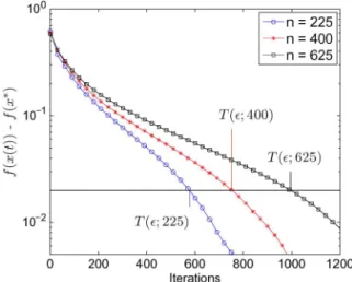
Fig. 2. Plot of the function error versus the number of iterations for a grid graph (see text).
To show that the statement holds with high probability when is compact and , it is sufficient to establish that the sequence is a bounded difference martingale and apply Azuma’s inequality [31]. (Under com-pactness and bounded norm conditions, our previous bounds on terms in the decomposition (45) now hold for the analogous terms in the decomposition (46) without taking expectations.)
By assumption on the compactness of and the Lipschitz assumptions on , we have
Recalling (47), we conclude that the last sum in the decompo-sition (46) is a bounded difference martingale, and Azuma’s in-equality implies that
Dividing by and setting the probability above to , we obtain
with probability at least .
The second statement of the theorem is now ob-tained by appealing to Lemma 4. By convexity, we have , thereby completing the proof.
IX. SIMULATIONS
In this section, we report experimental results on the conver-gence behavior of the distributed dual averaging algorithm as a function of the graph structure and number of nodes as well as giving comparison of distributed dual averaging to the methods in [10] and [11]. These results illustrate the excellent agreement of the empirical behavior with our theoretical predictions and improved algorithmic performance.
For all experiments reported here, we consider distributed minimization of a sum of -regression loss functions; these are robust versions of standard linear regression and useful in
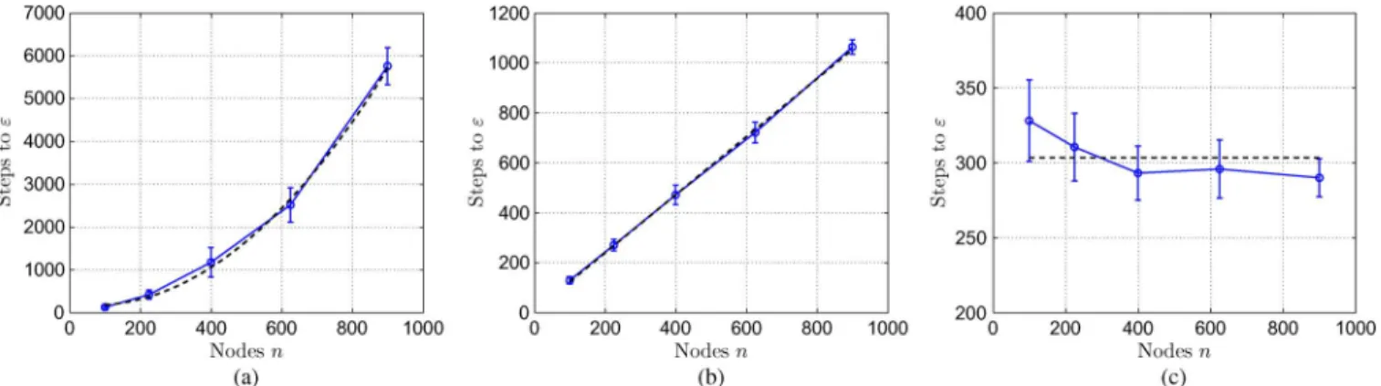
Fig. 3. Each plot shows the number of iterations required to reach afixed accuracy (vertical axis) versus the network size (horizontal axis). Each panel shows the same plot for a different graph topology: (a) single cycle; (b) two-dimensional grid; and (c) bounded degree expander. Step sizes were chosen according to the spectral gap. Dotted lines show predictions of Corollary 1.
system identification [32]. In this problem, we are given pairs of the form and whish to estimate a vector that so that . That is, we minimize
(48) Setting , we note that is -Lipschitz and non-smooth at any point with . It is common to impose some type of norm constraint on the solution of (48), so we set . For a given graph size , we form a random instance of a regression problem with data points. In order to study the effect of graph size and topology, we perform simulations with three different graph structures, namely cycles, grids, and random 5-regular expanders [23]. In all cases, we use the setting of the step size specified in Theorem 2 and Corollary 1.
Fig. 2 provides a plot of the function error
versus the number of iterations for grid graphs with a varying number of nodes . In addition to demonstrating convergence, the plots also shows how the con-vergence time scales as a function of the graph size . For any
fixed , the function defined in (11) shifts to the right as is increased, and our analysis aims to gain a precise understanding of this shifting.
In Fig. 3, we compare our theoretical predictions with the ac-tual behavior of dual subgradient averaging. Each panel shows the function versus the graph size for thefixed value ; the three different panels correspond to different graph types: cycles (a), grids (b), and expanders (c). In each panel, each point on the heavy blue curve is the average of 20 trials, and the bars show standard errors. For comparison, the dotted black line shows the theoretical prediction of Corollary 1. Note the excellent agreement between the empirical behavior and the-oretical predictions in all cases. In particular, panel (a) exhibits the quadratic scaling predicted for the cycle, panel (b) exhibits the the linear scaling expected for the grid, and panel (c) shows that expander graphs have the desirable property of constant net-work scaling.
Our final set of experiments compares the distributed dual averaging method (DDA) that we present to the Markov in-cremental gradient descent (MIGD) method [11] and the dis-tributed projected gradient method [10]. In Fig. 4, we plot the
Fig. 4. Number of iterations for distributed dual averaging (DDA) and Markov incremental gradient descent (MIGD) [11] to reachfixed accuracy versus net-work size for (a) two-dimensional grids and (b) bounded degree expanders.
quantity versus graph size for DDA and MIGD on grid and expander graphs. We use the optimal stepsize sug-gested by the analyses for each method. (We do not plot results for the distributed projected gradient method [10] because the optimal choice of stepsize according to the analysis therein re-sults in such slow convergence that it does notfit on the plots.) Fig. 4 makes it clear that—especially on graphs with good con-nectivity properties—the dual averaging algorithm gives im-proved performance.
X. CONCLUSION ANDDISCUSSION
In this paper, we proposed and analyzed a distributed dual av-eraging algorithm for minimizing the sum of local convex func-tions over a network. It is computationally efficient, and we pro-vided a sharp analysis of its convergence behavior as a function of the properties of the optimization functions and the underlying network topology. Our analysis demonstrates a close connection between convergence rates and mixing times of random walks on the underlying graph; such a connection is natural given the local and graph-constrained nature of our updates. In addition to anal-ysis of deterministic updates, our results also include stochastic communication protocols, for instance when communication oc-curs only along a random subset of the edges at each round. Such extensions allow for the design of protocols that tradeoff amount of communication and convergence rate. We also demonstrate that our algorithm is robust to noise by providing an analysis for the case of stochastic optimization with noisy gradients. We
con-firmed the sharpness of our theoretical predictions by implemen-tation and simulation of our algorithm.
There are several interesting open questions that remain to be explored. For instance, it would be interesting to analyze the convergence properties of other kinds of network-based opti-mization problems, by combining local information in different structures. It would also be of interest to study what other opti-mization procedures from the standard setting can be converted into efficient distributed algorithms to better exploit problem structure when possible.
ACKNOWLEDGMENT
The authors would like to thank the several anonymous re-viewers and John Tsitsiklis for their careful reading and helpful comments.
REFERENCES
[1] D. P. Bertsekas and J. N. Tsitsiklis, Parallel and Distributed Compu-tation: Numerical Methods. New York: Prentice-Hall, 1989. [2] Distributed Sensor Networks: A Multiagent Perspective, V. Lesser, C.
Ortiz, and M. Tambe, Eds. Norwell, MA: Kluwer, 2003, vol. 9. [3] D. Li, K. Wong, Y. Hu, and A. Sayeed, “Detection, classification
and tracking of targets in distributed sensor networks,”IEEE Signal Process. Mag., vol. 19, no. 2, pp. 17–29, Mar. 2002.
[4] L. Xiao, S. Boyd, and S. J. Kim, “Distributed average consensus with least-mean-square deviation,”J. Parallel Distrib. Comput., vol. 67, no. 1, pp. 33–46, 2007.
[5] C. Cortes and V. Vapnik, “Support-vector networks,”Mach. Learn., vol. 20, no. 3, pp. 273–297, Sep. 1995.
[6] J. Tsitsiklis, “Problems in decentralized decision making and compu-tation,” Ph.D. dissertation, Mass. Inst. of Technol., Cambridge, 1984. [7] J. N. Tsitsiklis, D. P. Bertsekas, and M. Athans, “Distributed
asynchronous deterministic and stochastic gradient optimization algo-rithms,”IEEE Trans. Autom. Control, vol. AC-31, no. 9, pp. 803–812, Sep. 1986.
[8] A. Nedićand A. Ozdaglar, “Distributed subgradient methods for multi-agent optimization,”IEEE Trans. Autom. Control, vol. 54, no. 1, pp. 48–61, Jan. 2009.
[9] I. Lobel and A. Ozdaglar, “Distributed subgradient methods over random networks,” MIT LIDS, Tech. Rep. 2800, 2009.
[10] S. S. Ram, A. Nedić, and V. V. Veeravalli, “Distributed stochastic sub-gradient projection algorithms for convex optimization,”J. Optimiz. Theory Applicat., vol. 147, no. 3, pp. 516–545, 2010.
[11] B. Johansson, M. Rabi, and M. Johansson, “A randomized incre-mental subgradient method for distributed optimization in networked systems,”SIAM J. Optimiz., vol. 20, no. 3, pp. 1157–1170, 2009. [12] A. Nedić, A. Olshevsky, A. Ozdaglar, and J. N. Tsitsiklis, “On
dis-tributed averaging algorithms and quantization effects,”IEEE Trans. Autom. Control, vol. 54, no. 11, pp. 2506–2517, Nov. 2009. [13] Y. Nesterov, “Primal-dual subgradient methods for convex problems,”
Math. Program. A, vol. 120, no. 1, pp. 261–283, 2009.
[14] L. Xiao, “Dual averaging methods for regularized stochastic learning and online optimization,”J. Mach. Learn. Res., vol. 11, pp. 2543–2596, 2010.
[15] J. Hiriart-Urruty and C. Lemaréchal, Convex Analysis and Minimiza-tion Algorithms I & II. New York: Springer, 1996.
[16] A. Kalai and S. Vempala, “Efficient algorithms for online decision problems,”J. Comput. Syst. Sci., vol. 71, no. 3, pp. 291–307, 2005. [17] R. A. Horn and C. R. Johnson, Matrix Analysis. Cambridge, U.K.:
Cambridge Univ. Press, 1985.
[18] D. Levin, Y. Peres, and E. Wilmer, Markov Chains and Mixing Times. Providence, RI: Amer. Math. Soc., 2008.
[19] P. Gupta and P. Kumar, “The capacity of wireless networks,”IEEE Trans. Inf. Theory, vol. 46, no. 2, pp. 388–404, Mar. 2000.
[20] M. Penrose, Random Geometric Graphs. New York: Oxford Univer-sity Press, 2003.
[21] F. Chung, Spectral Graph Theory. Providence, RI: Amer. Math. Soc., 1998.
[22] N. Alon, “Eigenvalues and expanders,” Combinatorica, vol. 6, pp. 83–96, 1986.
[23] J. Friedman, J. Kahn, and E. Szemerédi, “On the second eigenvalue of random regular graphs,” inProc. 21st Annu. ACM Symp. Theory Comput., 1989, pp. 587–598, ACM.
[24] A. Nemirovski and D. Yudin, Problem Complexity and Method Effi -ciency in Optimization. New York: Wiley, 1983.
[25] S. Boyd, A. Ghosh, B. Prabhakar, and D. Shah, “Randomized gossip algorithms,”IEEE Trans. Inf. Theory, vol. 52, no. 6, pp. 2508–2530, Jun. 2006.
[26] J. Duchi, A. Agarwal, and M. Wainwright, “Dual averaging for distributed optimization: convergence analysis and network scaling,” 2011 [Online]. Available: http://arxiv.org/abs/1005.2012
[27] D. Mosk-Aoyama, T. Roughgarden, and D. Shah, “Fully distributed algorithms for convex optimization problems,”SIAM J. Optimiz., vol. 20, no. 6, pp. 3260–3279, 2010.
[28] R. Gray, “Toeplitz and circulant matrices: A review,”Found. Trends Commun. Inf. Theory, vol. 2, no. 3, pp. 155–239, 2006.
[29] U. von Luxburg, A. Radl, and M. Hein, “Hitting times, commute dis-tances, and the spectral gap for large random geometric graphs,” 2010 [Online]. Available: http://arxiv.org/abs/1003.1266
[30] A. Olshevsky and J. N. Tsitsiklis, “A lower bound on distributed averaging,” in Proc. 49th IEEE Conf. Decision Control, 2010, pp. 4523–4528.
[31] K. Azuma, “Weighted sums of certain dependent random variables,”
Tohoku Math. J., vol. 68, pp. 357–367, 1967.
[32] B. T. Polyak and J. Tsypkin, “Robust identification,”Automatica, vol. 16, pp. 53–63, 1980.
John C. Duchireceived the B.S. and M.S. degrees in computer science from Stanford University, Stanford, CA, in 2007. He is currently pursuing the Ph.D. degree in computer science at the University of California, Berkeley.
Mr. Duchi received the National Defense Science and Engineering Graduate Fellowship in 2009, and has won a best paper award at the 2010 International Conference on Machine Learning.
Alekh Agarwalreceived the B.Tech degree in computer science and engi-neering from the Indian Institute of Technology Bombay, Mumbai, India in 2007, and the M.A. degree in statistics from the University of California, Berkeley, in 2009 where he is currently pursuing the Ph.D. degree in computer science.
Mr. Agarwal received the Microsoft Research Fellowship in 2009 and a Google Fellowship in 2011.
Martin J. Wainwright(M’03–SM’10) received the B.S. degree in mathematics from the University of Waterloo, Waterloo, ON, Canada, and the Ph.D. degree in electrical engineering and computer science (EECS) from the Massachusetts Institute of Technology (MIT), Cambridge.
He is currently a Professor at the University of California at Berkeley, with a joint appointment between the Department of Statistics and the Department of Electrical Engineering and Computer Sciences. His research interests include coding and information theory, machine learning, mathematical statistics, and statistical signal processing.
Prof. Wainwright has been awarded an Alfred P. Sloan Foundation Fellow-ship, an NSF CAREER Award, the George M. Sprowls Prize for his dissertation research (EECS Department, MIT), a Natural Sciences and Engineering Re-search Council of Canada 1967 Fellowship, an IEEE Signal Processing Society Best Paper Award in 2008, and several outstanding conference paper awards.