Probabilistic Programming for Deep Learning
Dustin Tran
Submitted in partial fulfillment of the requirements for the degree of
Doctor of Philosophy under the Executive Committee of the Graduate School of Arts and Sciences
COLUMBIA UNIVERSITY
© 2020
Dustin Tran
Abstract
Probabilistic Programming for Deep Learning
Dustin Tran
We propose the idea ofdeep probabilistic programming, a synthesis of advances for systems at the intersection of probabilistic modeling and deep learning. Such systems enable the development of new probabilistic models and inference algorithms that would otherwise be impossible: enabling unprecedented scales to billions of parameters, distributed and mixed precision environments, and AI accelerators; integration with neural architectures for modeling massive and high-dimensional datasets; and the use of computation graphs for automatic differentiation and arbitrary manipulation of probabilistic programs for flexible inference and model criticism.
After describing deep probabilistic programming, we discuss applications in novel variational inference algorithms and deep probabilistic models. First, we introduce the variational Gaussian process (vgp), a Bayesian nonparametric variational family, which adapts its shape to match complex posterior distributions. The vgp generates approximate posterior samples by generating latent inputs and warping them through random non-linear mappings; the distribution over random mappings is learned during inference, enabling the transformed outputs to adapt to varying complexity of the true posterior. Second, we introduce hierarchical implicit models (hims). hims combine the idea of implicit densities with hierarchical Bayesian modeling, thereby defining models via simulators of data with rich hidden structure.
Table of Contents
List of Tables . . . . vi
List of Figures . . . . vii
Acknowledgments . . . . xi
Chapter 1: Introduction, Background, & History . . . . 1
1.1 Probabilistic Machine Learning. . . 1
1.1.1 Probabilistic Models . . . 3
1.1.2 Inference of Probabilistic Models . . . 3
1.1.3 Variational Inference . . . 4
1.1.4 Maximum a Posteriori Estimation . . . 4
1.1.5 Laplace Approximation. . . 6
1.1.6 KL(qkp)Minimization . . . 6
1.1.7 Model Criticism . . . 9
1.2 History of probabilistic systems . . . 11
Chapter 2: Deep Probabilistic Programming . . . . 13
2.1 Introduction . . . 13
2.2 Compositional Representations for Probabilistic Models. . . 14
2.2.2 Example: Bayesian Recurrent Neural Network with Variable Length . . . . 16
2.2.3 Stochastic Control Flow and Model Parallelism . . . 16
2.3 Compositional Representations for Inference . . . 17
2.3.1 Inference as Stochastic Graph Optimization . . . 18
2.3.2 Classes of Inference . . . 19
2.3.3 Composing Inferences . . . 21
2.3.4 Data Subsampling . . . 21
2.4 Experiments . . . 22
2.4.1 Recent Methods in Variational Inference. . . 23
2.4.2 GPU-accelerated Hamiltonian Monte Carlo . . . 24
2.5 Discussion. . . 25
Chapter 3: Simple, Distributed, and Accelerated Probabilistic Programming . . . . 26
3.1 Introduction . . . 26
3.2 Random Variables Are All You Need. . . 27
3.2.1 Probabilistic Programs, Variational Programs, and Many More . . . 27
3.2.2 Example: Model-Parallel VAE with TPUs . . . 29
3.2.3 Tracing . . . 29
3.2.4 Tracing Applications . . . 32
3.3 Examples: Learning with Low-Level Functions . . . 32
3.3.1 Example: Data-Parallel Image Transformer with TPUs . . . 33
3.3.2 Example: No-U-Turn Sampler . . . 34
3.3.3 Example: Alignment of Probabilistic Programs . . . 35
3.3.4 Example: Learning to Learn by Variational Inference by Gradient Descent. 35 3.4 Experiments . . . 36
3.4.1 High-Quality Image Generation . . . 36
3.4.2 No-U-Turn Sampler. . . 38
3.5 Discussion. . . 38
Chapter 4: Applications in Variational Inference . . . . 40
4.1 Introduction . . . 40
4.2 Variational Gaussian Process . . . 41
4.2.1 Variational models . . . 41
4.2.2 Gaussian Processes . . . 42
4.2.3 Variational Gaussian Processes. . . 43
4.2.4 Universal approximation theorem . . . 45
4.3 Black box inference . . . 46
4.3.1 Variational objective . . . 46
4.3.2 Auto-encoding variational models . . . 47
4.3.3 Stochastic optimization . . . 48
4.3.4 Computational and storage complexity. . . 49
4.4 Experiments . . . 50
4.4.1 Binarized MNIST. . . 50
4.4.2 Sketch. . . 51
4.5 Discussion. . . 52
Chapter 5: Applications in Deep Probabilistic Models . . . . 53
5.1 Introduction . . . 53
5.2 Hierarchical Implicit Models . . . 54
5.3.1 KL Variational Objective. . . 58
5.3.2 Ratio Estimation for the KL Objective . . . 58
5.3.3 Stochastic Gradients of the KL Objective . . . 59
5.3.4 Algorithm. . . 61
5.4 Experiments . . . 62
5.5 Discussion. . . 65
References . . . . 81
Appendix A: Deep Probabilistic Programming . . . . 82
A.1 Model Examples . . . 82
A.2 Bayesian Neural Network for Classification . . . 82
A.3 Latent Dirichlet Allocation . . . 82
A.4 Gaussian Matrix Factorizationn. . . 83
A.5 Dirichlet Process Mixture Model . . . 83
A.6 Inference Example: Stochastic Variational Inference. . . 84
A.7 Complete Examples . . . 86
A.8 Variational Auto-encoder . . . 86
A.9 Probabilistic Model for Word Embeddings . . . 86
Appendix B: Simple, Distributed, and Accelerated Probabilistic Programming . . . . 89
B.1 Edward2 on SciPy. . . 89
B.2 Grammar Variational Auto-Encoder . . . 90
B.3 Markov chain Monte Carlo within Variational Inference . . . 92
Appendix C: Applications in Variational Inference . . . . 95
C.1 Special cases of the variational Gaussian process . . . 95
C.2 Proof of Theorem 1 . . . 96
C.3 Variational objective . . . 97
C.4 Gradients of the variational objective . . . 99
C.5 Scaling the size of variational data . . . 100
Appendix D: Applications in Probabilistic Models . . . . 101
D.1 Noise versus Latent Variables. . . 101
D.2 Implicit Model Examples in Edward . . . 102
D.3 KL Uniqueness . . . 102
D.4 Hinge Loss . . . 104
D.5 Comparing Bayesian GANs with MAP to GANs with MLE . . . 104
List of Tables
2.1 Inference methods for a probabilistic decoder on binarized MNIST. The Edward probabilistic programming language (ppl) is a convenient research platform, making it easy to both develop and experiment with many algorithms.. . . 23 2.2 Hamiltonian Monte Carlo (hmc) benchmark for large-scale logistic regression.
Ed-ward (GPU) is significantly faster than other systems. In addition, EdEd-ward has no overhead: it is as fast as handwritten TensorFlow. . . 24
3.1 Time per leapfrog step for No-U-Turn Sampler in Bayesian logistic regression. Ed-ward2 (GPU) achieves a 37x speedup over PyMC3 (CPU); dynamism is not available in Edward. Edward2 also incurs negligible overhead over handwritten TensorFlow code. . . 37
4.1 Negative predictive log-likelihood for binarized MNIST. Previous best results are [1] (Burda et al., 2016a), [2] (Salimans et al., 2015), [3] (Rezende and Mohamed, 2015), [4] (Raiko et al., 2014), [5] (Murray and Salakhutdinov, 2009), [6] (Gregor et al., 2014), [7] (Gregor et al., 2015). . . 51 4.2 Negative predictive log-likelihood for Sketch, learned over hundreds of epochs over
all 18,000 training examples. . . 52
5.1 Classification accuracy of Bayesian generative adversarial network (gan) and Bayesian neural networks across small to medium-size data sets. Bayesian gans achieve com-parable or better performance to their Bayesian neural net counterpart. . . 63
List of Figures
1.1 Box’s loop. . . 2 1.2 Distribution of test statistic replicated over generated datasets, along with the test
statistic applied to the observed dataset. . . 11
2.1 Beta-Bernoulli program(left)alongside its computational graph(right). Fetchingx from the graph generates a binary vector of50elements. . . 14 2.2 Variational auto-encoder for a data set of28×28pixel images: (left)graphical model,
with dotted lines for the inference model;(right)probabilistic program, with 2-layer neural networks. . . 15 2.3 Bayesian recurrent neural network (rnn): (left)graphical model;(right)probabilistic
program. The program has an unspecified number of time steps; it uses a symbolic for loop (tf.scan).. . . 17 2.4 Computational graph for a probabilistic program with stochastic control flow. . . . 17 2.5 Hierarchical model: (left) graphical model;(right)probabilistic program. It is a
mixture of Gaussians overD-dimensional data{xn} ∈RN×D. There areK latent cluster meansβ∈RK×D. . . 18 2.6 (left)Variational inference.(right)Monte Carlo. . . 19 2.7 Generative adversarial networks: (left)graphical model;(right)probabilistic
pro-gram. The model (generator) uses a parameterized function (discriminator) for training. . . 20 2.8 Combining inference algorithms to perform variational EM. . . 21 2.9 Data subsampling with a hierarchical model. We define a subgraph of the full model,
forming a plate of sizeM rather thanN. We then scale all local random variables by
N/M. . . 22 2.10 Edward program for Bayesian logistic regression with hmc. . . 24
3.1 Beta-Bernoulli program. In eager mode,model()generates a binary vector of50 elements. In graph mode,model()returns an op to be evaluated in a TensorFlow session. . . 28 3.2 Variational program (Ranganath et al., 2016a), available in eager mode. Python
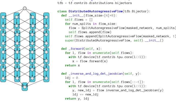
control flow is applicable to generative processes: given a coin flip, the program generates from one of two neural nets. Their outputs can have differing shape (and structure). . . 28 3.3 Distributed autoregressive flows.(right)The default length is 8, each with 4
indepen-dent flows. Each flow transforms inputs via layers respecting autoregressive ordering.
(left)Flows are partitioned across a virtual topology of 4x4 cores (rectangles); each core computes 2 flows and is locally connected; a final core aggregates. The virtual topology aligns with the physical tensor processing unit (tpu) topology: for 4x4 tpus, it is exact; for 16x16 tpus, it is duplicated for data parallelism. . . 30 3.4 Model-parallel variational auto-encoder (vae) with tpus, generating 16-bit audio
from 8-bit latents. The prior and decoder split computation according to distributed autoregressive flows. The encoder may split computation according tocompressor; we omit it for space.. . . 30 3.5 Minimal implementation of tracing. tracedefines a context; any traceable ops
executed during it are replaced by calls totracer. traceableregisters these ops; we register Edward random variables. . . 31 3.6 A program execution. It is a directed acyclic graph and is traced for various operations
such as accumulating log-probabilities or finding conditional independence. . . 31 3.7 A higher-order function which takes amodelprogram as input and returns its log-joint
density function. . . 31 3.8 A higher-order function which takes amodelprogram as input and returns its causally
intervened program. Intervention differs from conditioning: it does not change the sampled value but the distribution. . . 31 3.9 Data-parallel Image Transformer with tpus (Parmar et al., 2018). It is a neural
autoregressive model which computes the log-probability of a batch of images with self-attention. Our lightweight design enables representing and training the model as a log-probability function; this is more efficient than the typical representation of programs as a generative process. Embedding and self-attention functions are assumed in the environment; they are available in Tensor2Tensor (Vaswani et al., 2018). . . 33 3.10 Core logic in No-U-Turn Sampler (Hoffman and Gelman, 2014). This algorithm has
3.11 Learning often involves matching two execution traces such as a model program’s
(left)and a variational program’s(right), or a model program’s with data tensors
(bot-tom). Red arrowsalign prior and variational variables. Blue arrows align observed variables and data; edges from data to variational variables represent amortization. 34 3.12 Variational inference with preconditioned gradient descent. Edward2 offers writing
the probabilistic program and performing arbitrary TensorFlow computation for
learning. . . 36
3.13 Learning-to-learn. It finds the optimal preconditioner fortrain(Figure 3.12) by differentiating the entire learning algorithm with respect to the preconditioner. . . 36
3.14 Vector-Quantized VAE on 64x64 ImageNet. . . 37
3.15 Image Transformer on 256x256 CelebA-HQ. . . 37
4.1 (a)Graphical model of the variational Gaussian process. The vgp generates samples of latent variables z by evaluating random non-linear mappings of latent inputs ξ, and then drawing mean-field samples parameterized by the mapping. These latent variables aim to follow the posterior distribution for a generative model(b), conditioned on datax. . . 44
4.2 Sequence of domain mappings during inference, from variational latent variable spaceRto posterior latent variable spaceQto data spaceP. We perform variational inference in the posterior space and auxiliary inference in the variational space. . . 46
4.3 Generated images from Deep Recurrent Attentive Writer (draw) with a vgp (top), and draw with the original variational auto-encoder (bottom). The vgp learns texture and sharpness, able to sketch more complex shapes. . . 52
5.1 (left) Hierarchical model, with local variablesz and global variables β. (right) Hierarchical implicit model. It is a hierarchical model wherexis a deterministic function (denoted with a square) of noise(denoted with a triangle). . . 55
5.2 (top) Marginal posterior for first two parameters. (bot. left)ABC methods over tolerance error. (bot. right)Marginal posterior for first parameter on a large-scale data set. Our inference achieves more accurate results and scales to massive data. . 62
A.1 Bayesian neural network for classification. . . 83
A.2 Latent Dirichlet allocation (Blei et al., 2003). . . 83
A.3 Gaussian matrix factorization. . . 83
A.5 Complete script for a vae (Kingma and Welling, 2014b) with batch training. It generates MNIST digits after every 1000 updates. . . 87 A.6 Exponential family embedding for binary data (Rudolph et al., 2016). Here, maximum
a posteriori (map) is used to maximize the total sum of conditional log-likelihoods and log-priors.. . . 88
D.1 Two-layer deep implicit model for data pointsxn∈R10. The architecture alternates with stochastic and deterministic layers. To define a stochastic layer, we simply inject noise by concatenating it into the input of a neural net layer.. . . 102 D.2 Bayesian gan for classification, takingX∈RN×500as input and generating a vector
of labelsy∈ {−1,1}N. The neural network directly generates the data rather than parameterizing a probability distribution. . . 103 D.3 (left) Difference of ratios over steps of q. Low variance on y-axis means more
stable. Interestingly, the ratio estimator is more accurate and stable asqconverges to the posterior. (middle)Difference of ratios over steps ofr;qis fixed at random initialization. The ratio estimator doesn’t improve even after many steps. (right) Difference of ratios over steps ofr;qis fixed at the posterior. The ratio estimator only requires few steps from random initialization to be highly accurate. . . 106
Acknowledgments
I would like to acknowledge a number of people that supported this work.
First, I’d like to thank my advisor Prof. David Blei. I could not have hoped for an advisor with a greater overlap in research vision and clarity of thinking. Across our many works together, Dave gave me the opportunity to work with dozens of collaborators across university departments and outside university, across seniority levels, and across different yet similar research interests; this diversity made me a more successful researcher. I also admire that Dave is respectful, caring, and inviting: he shows by example how to be a better human being, and I’ve grown all the more for it.
I would like to sincerely thank Profs. Edo Airoldi and Finale Doshi-Velez during my formative years as I transitioned to a Ph.D. I especially thank my labmate Panos Toulis who graciously gave me experience on my first research publication. My earliest research projects could not have been successful without all their support.
At Columbia, I would like to thank my labmates: Rajesh Ranganath, Alp Kucukelbir, Adji Dieng, Maja Rudolph, Jaan Altosaar, Dawen Liang, Stephan Mandt, James McInerney, Fran Ruiz, and Christian Naesseth. I especially thank Rajesh for weathering all my idea pitching, frequent late-night research discussions, and frantic rushes for deadlines. I would like to thank Alp for helping me work on larger projects, iterate on research ideas, and become a better writer and coder. I enjoyed our frequent lunches in the Philosophy Hall. I shared a number of travels with Rajesh and Alp, and it’s always been a pleasure discussing ideas with them.
me to the Stan team, and in our many conversations. Aki Vehtari, Bob Carpenter, and Daniel Lee have all influenced how I approach applications and software. I especially thank Alp for being inviting as we worked together on variational inference for Stan. I would also like to thank Matt Hoffman for hosting me at Adobe Research (later, Google) to work on Edward.
Finally, I’d like to thank, and dedicate this work to, my parents Van and Mai for their continuing support as well as my two brothers Daniel and Dalton. My parents overcame great hardship as refugees in the United States, and I admire them for their dedication to make their children educated and successful.
Chapter 1: Introduction, Background, & History
Probabilistic modeling is a powerful approach for analyzing empirical information using foundations from probability theory (Tukey,1962;Newell and Simon,1976;Box,1976). Probabilistic models are an essential element of machine learning (Murphy,2012;Goodfellow et al.,2016) and statistics (Friedman et al.,2001;Gelman et al.,2013), featuring applications across fields such as compu-tational biology (Friedman et al.,2000), computational neuroscience (Dayan and Abbott,2001), cognitive science (Tenenbaum et al.,2011), information theory (MacKay,2003), and natural language processing (Manning and Schütze,1999).
In this thesis, we propose the idea ofdeep probabilistic programming, a synthesis of advances for the design and implementation of systems at the intersection of probabilistic modeling and deep learning. Such systems enable the development of new probabilistic models and inference algorithms that would otherwise be impossible: enabling unprecedented scales to billions of parameters, distributed and mixed precision environments, and AI accelerators; integration and flexibility with neural architectures for modeling massive and high-dimensional datasets; and the use of computation graphs for automatic differentiation and arbitrary manipulation of probabilistic programs for flexible inference algorithms and model criticism strategies.
Below we provide background in the probabilistic approach to machine learning as well as history behind probabilistic systems for their research and eventual deployment.Chapter 2andChapter 3
describes the design of deep probabilistic programming systems.Chapter 4andChapter 5discuss applications in novel probabilistic inference strategies as well as novel model classes.
1.1 Probabilistic Machine Learning
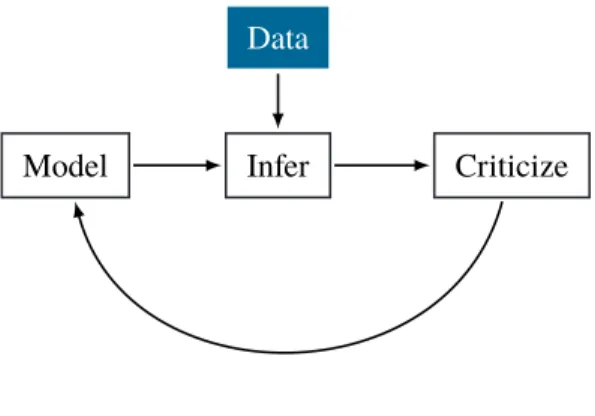
The process of data analysis in machine learning and statistics reflects that of the scientific method. Namely, there are core building blocks—interchangeable components which enable rapid iteration
Model Infer Data
Criticize
Figure 1.1:Box’s loop.
as they build on one another. These building blocks form a cycle that leads to their individual improvements as the cycle is unrolled over time. To formalize this, we follow a philosophy of statistics and machine learning known as Box’s loop (Box,1976;Blei,2014). Given a phenomena of interest:
1. Build a probabilistic model. The model formalizes a hypothesis about the phenomena using the language of probability.
2. Reason about the phenomena given model and gathered data. This data may come from designing and running an experiment, or it may come from gathering data that already exists (for example, previous experiments, or content such as text or images on the internet).
3. Criticize the model’s fit to the data, that is, how well the hypothesis empirically reflects the phenomena. Revise and repeat.
As an illustration, suppose a child flips a coin ten times, with the set of outcomes being
[0, 1, 0, 0, 0, 0, 0, 0, 0, 1],
where0denotes tails and1denotes heads. She is interested in the probability that the coin lands heads. To analyze this, she first builds a “model”: suppose she assumes the coin flips are independent and land heads with the same probability. Second, she reasons about the phenomenon: she infers the model’s hidden structure (the unknown probability value) given data. Finally, she criticizes the model: she analyzes whether her model captures the real-world phenomenon of coin flips. If it doesn’t, then she may revise the model and repeat.
Next we more formally describe the three components of probabilistic models, inference, and criti-cism.
1.1.1 Probabilistic Models
A probabilistic model asserts how observations from a natural phenomenon arise. The model is ajoint
distributionp(x,z)of observed variablesxcorresponding to data, and latent variableszthat provide the hidden structure to generate fromx. The joint distribution factorizes into two components.
Thelikelihoodp(x|z)is a probability distribution that describes how any dataxdepend on the latent variablesz. The likelihood posits a data generating process, where the dataxare assumed drawn from the likelihood conditioned on a particular hidden pattern described byz. Theprior p(z)is a probability distribution that describes the latent variables present in the data. It posits a generating process of the hidden structure.
Ultimately, how the likelihood depends onzcan be incredibly complex in the real world: neural net-works are a common class of functions that enable parameterizing the likelihood for high-dimensional distributions, proven empirically to work well across perceptual tasks such as image classification (Krizhevsky et al.,2012). For the purposes of this thesis, we do not provide background on neural networks. Their specific architectures are not central to the thesis; we recommendGoodfellow et al.
(2016) as a survey.
1.1.2 Inference of Probabilistic Models
How can we use a modelp(x,z)to analyze gathered datax? In other words, what hidden structurez explains the data? We seek to infer this hidden structure using the model.
One method of inference leverages Bayes’ rule to define theposterior
p(z|x) = R p(x,z)
p(x,z)dz.
The posterior is the distribution of the latent variablesz, conditioned on the observed datax. It is a probabilistic description of the data’s hidden representation.
hypothesis about the latent variables, representing our new subjective belief about the phenomena. From the perspective of hypothetico-deductivism, as practiced by statisticians such as Box, Rubin, and Gelman, the posterior is simply a fitted model to data and thus a falsifiable hypothesis, to be criticized and ultimately revised (Box,1982;Gelman and Shalizi,2013).
Inferring the posterior. Now we know what the posterior represents. How do we calculate it? This is the central computational challenge in probabilistic inference. The posterior is difficult to compute because of its normalizing constant, which is the integral in the denominator. This is often a high-dimensional integral that lacks an analytic (closed-form) solution. Thus, calculating the posterior meansapproximatingthe posterior.
1.1.3 Variational Inference
Variational inference is an umbrella term for algorithms which cast posterior inference as optimization (Hinton and van Camp,1993;Waterhouse et al.,1996;Jordan et al.,1999a). The core idea involves two steps:
1. posit a family of distributionsq(z; λ)over the latent variables;
2. matchq(z; λ)to the posterior by optimizing over its parametersλ.
This strategy converts the problem of computing the posteriorp(z|x)into an optimization problem: minimize a loss function
λ∗= arg min
λ loss(p(z|x), q(z; λ)).
The optimized distributionq(z; λ∗)is used as a proxy to the posteriorp(z|x).
1.1.4 Maximum a Posteriori Estimation
One form of variational inference is known as maximum a posteriori (MAP) estimation. It uses the mode as a point estimate of the posterior distribution,
zMAP= arg max
Namely, the posited family of variational distributions are simply delta distributions with probability 1 at a point. In practice, we work with logarithms of densities to avoid numerical underflow issues (Murphy,2012).
The MAP estimate is the most likely configuration of the hidden patternszunder the model. However, we cannot directly solve this optimization problem because the posterior is typically intractable. To circumvent this, we use Bayes’ rule to optimize over the joint density,
zMAP= arg max
z logp(z|x) = arg maxz logp(x,z).
This is valid because
logp(z|x) = logp(x,z)−logp(x) = logp(x,z)−constant in terms ofz.
MAP estimation includes the common scenario of maximum likelihood estimation as a special case,
zMAP= arg max
z p(x,z) = arg maxz p(x|z),
where the prior p(z) is flat, placing uniform probability over all values z supports. Placing a nonuniform prior can be thought of as regularizing the estimation, penalizing values away from maximizing the likelihood, which can lead to overfitting. For example, a normal prior or Laplace prior onzcorresponds to`2penalization, also known as ridge regression, and`1penalization, also known as the LASSO.
Maximum likelihood is also known as cross entropy minimization. For a data setx={xn},
zMAP = arg max
z logp(x|z) = arg maxz
N
X
n=1
logp(xn|z) = arg min
z − 1 N N X n=1 logp(xn|z).
The last expression can be thought of as an approximation to the cross entropy between the true data distribution andp(x|z), using a set ofN data points.
joint density∇zlogp(x,z)and follow it to a (local) optima.
1.1.5 Laplace Approximation
Maximum a posteriori (MAP) estimation approximates the posteriorp(z|x)with a point mass (delta function) by simply capturing its mode. MAP is attractive because it is fast and efficient. How can we use MAP to construct a better approximation to the posterior?
The Laplace approximation (Laplace,1986) is one way of improving a MAP estimate. The idea is to approximate the posterior with a normal distribution centered at the MAP estimate,
p(z|x)≈Normal(z; zMAP,Λ −1).
This requires computing a precision matrix Λ. Derived from a Taylor expansion, the Laplace approximation uses the Hessian of the negative log joint density at the MAP estimate. It is defined component-wise as
Λij = ∂2 ∂zi∂zj
−logp(x,z).
For flat priors (which reduces MAP to maximum likelihood), the precision matrix is known as the observed Fisher information (Fisher,1925). Edward uses TensorFlow’s automatic differentiation, making this distribute.
1.1.6 KL(qkp)Minimization
MAP estimation and the Laplace approximation are simple, but make local and Gaussian assumptions in approximating the true posterior distribution. Another popular form of variational inference minimizes the Kullback-Leibler divergence fromq(z; λ)top(z|x),
λ∗ = arg min λ KL(q(z; λ)kp(z|x)) = arg min λ Eq(z;λ) logq(z; λ)−logp(z|x).
The KL divergence is a non-symmetric, information theoretic measure of similarity between two prob-ability distributions (Hinton and van Camp,1993;Waterhouse et al.,1996;Jordan et al.,1999a).
The Evidence Lower Bound. The above optimization problem is intractable because it directly depends on the posteriorp(z|x). To tackle this, consider the property
logp(x) =KL(q(z; λ)kp(z|x)) +Eq(z;λ)
logp(x,z)−logq(z; λ)
where the left hand side is the logarithm of the marginal likelihoodp(x) =Rp(x,z)dz, also known as the model evidence.
The evidence is a constant with respect to the variational parametersλ, so we can minimize KL(qkp) by instead maximizing theevidence lower bound(elbo),
ELBO(λ) = Eq(z;λ)
logp(x,z)−logq(z; λ)
.
In the elbo, bothp(x,z)andq(z; λ)are tractable. The optimization problem reduces to
λ∗ = arg max
λ ELBO(λ).
As per its name, the elbo is a lower bound on the evidence, and optimizing it tries to maximize the probability of observing the data. What does maximizing the elbo do? Splitting the elbo reveals a trade-off
ELBO(λ) = Eq(z;λ)[logp(x,z)]−Eq(z;λ)[logq(z; λ)],
where the first term represents an energy and the second term (including the minus sign) represents the entropy ofq. The energy encouragesq to focus probability mass where the model puts high probability,p(x,z). The entropy encouragesqto spread probability mass to avoid concentrating to one location.
There are two general strategies to obtain gradients for gradient-based optimization: score function gradient; and reparameterization gradient.
Score function gradient. Gradient descent is a standard approach for optimizing complicated objectives like the elbo. The idea is to calculate its gradient
∇λ ELBO(λ) =∇λEq(z;λ)
logp(x,z)−logq(z; λ)
,
and update the current set of parameters proportional to the gradient. The score function gradient estimator leverages a property of logarithms to write the gradient as
∇λ ELBO(λ) = Eq(z;λ)
∇λlogq(z; λ) logp(x,z)−logq(z; λ)
.
The gradient of the elbo is an expectation over the variational modelq(z; λ); the only new ingredient it requires is thescore function∇λlogq(z; λ)(Paisley et al.,2012b;Ranganath et al.,2014). We can use Monte Carlo integration to obtain noisy estimates of both the elbo and its gradient. The basic procedure follows these steps:
1. drawSsamples{zs}S1 ∼q(z; λ),
2. evaluate the argument of the expectation using{zs}S1, and
3. compute the empirical mean of the evaluated quantities.
A Monte Carlo estimate of the gradient is then
∇λ ELBO(λ)≈ 1 S S X s=1 logp(x,zs)−logq(zs; λ) ∇λlogq(zs; λ) .
This is an unbiased estimate of the actual gradient of the elbo.
Reparameterization gradient. If the model has differentiable latent variables, then it is generally advantageous to leverage gradient information from the model in order to better traverse the opti-mization space. One approach to doing this is the reparameterization gradient (Kingma and Welling,
2014a;Rezende et al.,2014).
Some variational distributionsq(z ; λ) admit useful reparameterizations. For example, we can reparameterize a normal distributionz∼Normal(µ,Σ)asz=µ+L, where∼Normal(0, I)and
Σ =LL>. In general, write this as
∼q(), z=z(; λ),
whereis a random variable that doesnotdepend on the variational parametersλ. The deterministic functionz(·;λ)encapsulates the variational parameters instead, and following the process is equivalent to directly drawingzfrom the original distribution.
The reparameterization gradient leverages this property to write the gradient as
∇λ ELBO(λ) = Eq()
∇λ logp(x,z(; λ))−logq(z(; λ) ; λ)
.
The gradient of the elbo is an expectation over the base distributionq(), and the gradient can be applied directly to the inner expression. We can use Monte Carlo integration to obtain noisy estimates of both the elbo and its gradient. The basic procedure follows these steps:
1. drawSsamples{s}S1 ∼q(),
2. evaluate the argument of the expectation using{s}S1, and
3. compute the empirical mean of the evaluated quantities.
A Monte Carlo estimate of the gradient is then
∇λ ELBO(λ)≈ 1 S S X s=1 ∇λ logp(x,z(s; λ))−logq(z(s; λ) ; λ) .
This is an unbiased estimate of the actual gradient of the elbo. Empirically, it exhibits lower variance than the score function gradient, leading to faster convergence in a large set of problems (Tran et al.,
2016b).
1.1.7 Model Criticism
We can never validate whether a model is true. In practice, “all models are wrong” (Box,1976). However, we can try to uncover where the model goes wrong. Model criticism helps justify the model as an approximation or point to good directions for revising the model.
Model criticism typically analyzes the posterior predictive distribution,
p(xnew|x) = Z
p(xnew|z)p(z|x)dz.
The model’s posterior predictive can be used to generate new data given past observations and can also make predictions on new data given past observations. It is formed by calculating the likelihood of the new data, averaged over every set of latent variables according to the posterior distribution.
Scoring rules. A scoring rule is a scalar-valued metric for assessing trained models (Winkler,1994;
Gneiting and Raftery,2007). For example, we can assess models for classification by predicting the label for each observation in the data and comparing it to their true labels. Formally, given two distributionspandqover a space of eventsx,
S(p, q) = Z
q(x)S(p, x)dx,
whereS(p, x)is a real-valued function of a densitypoverxsuch as the logarithmic scoring rule (logp(x)). It is common practice to criticize models with data held-out from training. In machine learning, benchmark datasets involve a train and test split.
Posterior predictive checks. Posterior predictive checks (PPCs) analyze the degree to which data generated from the model deviate from data generated from the true distribution. They can be used either numerically to quantify this degree, or graphically to visualize this degree. PPCs can be thought of as a probabilistic generalization of scoring rules, providing a distribution rather than a single value (Box,1980;Rubin,1984;Meng,1994;Gelman et al.,1996).
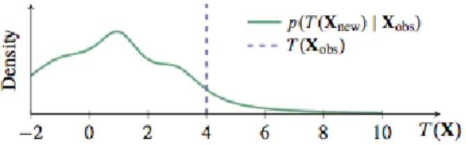
The simplest PPC works by applying a test statistic on replicated datasets generated from the posterior predictive, such as T(xnew) = max(xnew). Applying T(xnew) to new datasets over many data replications induces a distribution. We compare this distribution to the test statistic on the real data T(x).
InFigure 1.2,T(x)falls in a low probability region of this reference distribution: if the model were true, the probability of observing the test statistic is very low. This indicates that the model fits the data poorly according to this check; this suggests an area of improvement for the model.
Figure 1.2: Distribution of test statistic replicated over generated datasets, along with the test statistic applied to the observed dataset.
More generally, the test statistic can be a function of the model’s latent variablesT(x,z), known as a discrepancy function. Examples of discrepancy functions are the metrics used for scoring rules. We can now interpret the scoring rule as a special case of PPCs: it simply calculatesT(x,z)over the real data and without a reference distribution in mind. A reference distribution allows us to make probabilistic statements about the point, in reference to an overall distribution.
PPCs are an excellent tool for revising models—simplifying or expanding the current model as one examines its fit to data. They are inspired by classical hypothesis testing such as goodness-of-fit-tests; these methods criticize models under the frequentist perspective of large sample assessment.
PPCs can also be applied to tasks such as hypothesis testing, model comparison, model selection, and model averaging. It’s important to note that while PPCs can be applied as a form of Bayesian hypothesis testing, hypothesis testing is generally not recommended: binary decision making from a single test is not as common a use case as the broader process of assimilating this information into future model revisions and diagnostics.
1.2 History of probabilistic systems
For examples of probabilistic software systems, we point to two early threads. The first is in artificial intelligence. Expert systems were designed from human expertise, which in turn enabled larger reasoning steps according to existing knowledge (Buchanan et al., 1969;Minsky, 1975). With connectionist models, the design focused on neuron-like processing units, which learn from experience; this drove new applications of artificial intelligence (Hopfield,1982;Rumelhart et al.,1988). As a second thread, we point to early work in statistical computing, where interest grew broadly out of efficient computation for problems in statistical analysis. The S language, developed by John Chambers and colleagues at Bell Laboratories (Becker and Chambers,1984;Chambers and Hastie,
1992), focused on an interactive environment for data analysis, with simple yet rich syntax to quickly turn ideas into software. It is a predecessor to the R language (Ihaka and Gentleman,1996). More targeted environments such as BUGS (Spiegelhalter et al.,1995), which focuses on Bayesian analysis of statistical models, helped launch the emerging field of probabilistic programming.
We are motivated to build on these early works in probabilistic systems—where in modern applications, new challenges arise in their design and implementation. We highlight two challenges. First, statistics and machine learning have made significant advances in the methodology of probabilistic models and their inference (e.g., Hoffman et al.(2013);Ranganath et al. (2014);Rezende et al. (2014)). For software systems to enable fast experimentation, we require rich abstractions that can capture these advances: it must encompass both a broad class of probabilistic models and a broad class of algorithms for their efficient inference. Second, researchers are increasingly motivated to employ complex probabilistic models and at an unprecedented scale of massive data (Bengio et al.,2013;
Ghahramani,2015;Lake et al.,2016). Thus we require an efficient computing environment that supports distributed training and integration of hardware such as (multiple) GPUs.
A core theme in probabilistic programming is automated inference, used in systems such as BUGS (Spiegelhalter et al.,1995) with a Gibbs sampler to more recent work such as Stan (Carpenter et al.,
2015) with the No-U-Turn Sampler (Hoffman and Gelman,2014) and Automatic Differentiation Variational Inference (Kucukelbir et al.,2017). In this thesis, we examine effectively the opposite theme: flexible, composable inference for research on the algorithms themselves. This use case fits well with machine learning research, where the challenge is to devise better models and algorithms that work on a variety of domains and scale—ultimately toward the goal of more intelligent systems. The theme of automated inference is useful for a separate audience: applied scientists and practioners. These purposes could fit well as a higher-level abstraction built on top of what we describe here in developing more composable and flexible systems.
Chapter 2: Deep Probabilistic Programming
2.1 Introduction
The nature of deep neural networks is compositional. Users can connect layers in creative ways, without having to worry about how to perform testing (forward propagation) or inference (gradient-based optimization, with back propagation and automatic differentiation).
In this chapter, we design compositional representations for probabilistic programming. Probabilistic programming lets users specify generative probabilistic models as programs and then “compile” those models down into inference procedures. Probabilistic models are also compositional in nature, and much work has enabled rich probabilistic programs via compositions of random variables (Goodman et al.,2012;Ghahramani,2015;Lake et al.,2016).
Less work, however, has considered an analogous compositionality for inference. Rather, many existing probabilistic programming languages treat the inference engine as a black box, abstracted away from the model. These cannot capture probabilistic inferences that reuse the model’s representation— a key idea in recent advances in variational inference (Kingma and Welling,2014b;Rezende and Mohamed,2015;Tran et al.,2016b), generative adversarial networks (Goodfellow et al.,2014), and also in more classic inferences (Dayan et al.,1995;Gutmann and Hyvärinen,2010).
We propose Edward1, a Turing-complete probabilistic programming language which builds on two compositional representations—one for random variables and one for inference. By treating inference as a first class citizen, on a par with modeling, we show that probabilistic programming can be as flexible and computationally efficient as traditional deep learning. For flexibility, we show how Edward makes it easy to fit the same model using a variety of composable inference methods, ranging from point estimation to variational inference to mcmc. For efficiency, we show how to integrate
1
SeeTran et al.(2016a) for details of the API. A companion webpage for this paper is available athttp://edwardlib. org/iclr2017. It contains more complete examples with runnable code.
Edward into existing computational graph frameworks such as TensorFlow (Abadi et al., 2016). Frameworks like TensorFlow provide computational benefits like distributed training, parallelism, vectorization, and GPU support “for free.” For example, we show on a benchmark task that Edward’s Hamiltonian Monte Carlo is many times faster than existing software. Further, Edward incurs no runtime overhead: it is as fast as handwritten TensorFlow.
2.2 Compositional Representations for Probabilistic Models
We first develop compositional representations for probabilistic models. We desire two criteria: (a) integration with computational graphs, an efficient framework where nodes represent operations on data and edges represent data communicated between them (Culler,1986); and (b) invariance of the representation under the graph, that is, the representation can be reused during inference.
Edward defines random variables as the key compositional representation. They are class objects with methods, for example, to compute the log density and to sample. Further, each random variable
xis associated to a tensor (multi-dimensional array)x∗, which represents a single samplex∗ ∼p(x). This association embeds the random variable onto a computational graph on tensors.
The design’s simplicity makes it easy to develop probabilistic programs in a computational graph framework. Importantly, all computation is represented on the graph. This enables one to compose random variables with complex deterministic structure such as deep neural networks, a diverse set of math operations, and third party libraries that build on the same framework. The design also enables compositions of random variables to capture complex stochastic structure.
As an illustration, we use a Beta-Bernoulli model,p(x, θ) = Beta(θ|1,1)Q50n=1Bernoulli(xn|θ), whereθis a latent probability shared across the 50 data pointsx∈ {0,1}50. The random variablex is 50-dimensional, parameterized by the random tensorθ∗. Fetching the objectxruns the graph: it simulates from the generative process and outputs a binary vector of50elements.
theta = Beta(a=1.0, b=1.0) x = Bernoulli(p=tf.ones(50) * theta) θ θ∗ tf.ones(50) x x ∗
Figure 2.1: Beta-Bernoulli program(left)alongside its computational graph(right). Fetchingx from the graph generates a binary vector of50elements.
zn xn θ φ N # Probabilistic model z = Normal(mu=tf.zeros([N, d]), sigma=tf.ones([N, d]))
h = Dense(256, activation='relu')(z)
x = Bernoulli(logits=Dense(28 * 28, activation=None)(h))
# Variational model
qx = tf.placeholder(tf.float32, [N, 28 * 28])
qh = Dense(256, activation='relu')(qx)
qz = Normal(mu=Dense(d, activation=None)(qh),
sigma=Dense(d, activation='softplus')(qh))
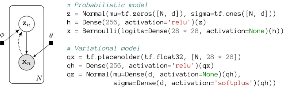
Figure 2.2: Variational auto-encoder for a data set of28×28pixel images:(left)graphical model, with dotted lines for the inference model;(right)probabilistic program, with 2-layer neural networks.
All computation is registered symbolically on random variables and not over their execution. Sym-bolic representations do not require reifying the full model, which leads to unreasonable memory consumption for large models (Tristan et al.,2014). Moreover, it enables us to simplify both de-terministic and stochastic operations in the graph, before executing any code (Ścibior et al.,2015;
Zinkov and Shan,2016).
With computational graphs, it is also natural to build mutable states within the probabilistic program. As a typical use of computational graphs, such states can define model parameters; in TensorFlow, this is given by atf.Variable. Another use case is for building discriminative modelsp(y|x), wherexare features that are input as training or test data. The program can be written independent of the data, using a mutable state (tf.placeholder) forxin its graph. During training and testing, we feed the placeholder the appropriate values.
InAppendix A.1, we provide examples of a Bayesian neural network for classification (A.2), latent Dirichlet allocation (A.3), and Gaussian matrix factorization (A.4). We present others below.
2.2.1 Example: Variational Auto-encoder
Figure 3.4implements a vae (Kingma and Welling,2014b;Rezende et al.,2014) in Edward. It comprises a probabilistic model over data and a variational model designed to approximate the former’s posterior. Here we use random variables to construct both the probabilistic model and the variational model; they are fit during inference (more details inSection 5.3).
There areN data pointsxn∈ {0,1}28·28each withdlatent variables,zn∈Rd. The program uses Keras (Chollet,2015) to define neural networks. The probabilistic model is parameterized by a 2-layer
neural network, with 256 hidden units (and ReLU activation), and generates28×28pixel images. The variational model is parameterized by a 2-layer inference network, with 256 hidden units and outputs parameters of a normal posterior approximation.
The probabilistic program is concise. Core elements of the vae—such as its distributional assumptions and neural net architectures—are all extensible. With model compositionality, we can embed it into more complicated models (Gregor et al.,2015;Rezende et al.,2016) and for other learning tasks (Kingma et al.,2014). With inference compositionality (which we discuss inSection 5.3), we can embed it into more complicated algorithms, such as with expressive variational approximations (Rezende and Mohamed,2015;Tran et al.,2016b;Kingma et al.,2016) and alternative objectives (Ranganath et al.,2016a;Li and Turner,2016;Dieng et al.,2016).
2.2.2 Example: Bayesian Recurrent Neural Network with Variable Length
Random variables can also be composed with control flow operations. As an example,Figure 2.3
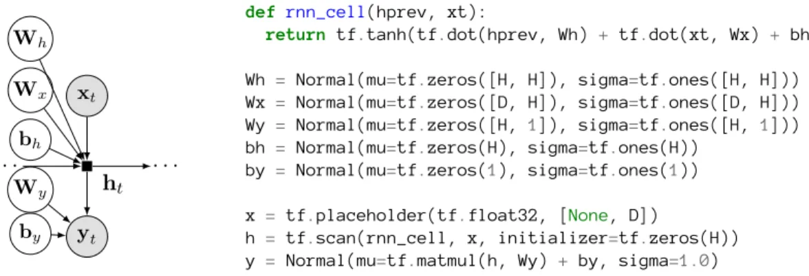
implements a Bayesian recurrent neural network (rnn) with variable length. The data is a sequence of inputs{x1, . . . ,xT}and outputs{y1, . . . , yT}of lengthT withxt ∈ RD andyt ∈ Rper time step. Fort= 1, . . . , T, a rnn applies the update
ht= tanh(Whht−1+Wxxt+bh),
where the previous hidden state isht−1 ∈RH. We feed each hidden state into the output’s likelihood, yt ∼Normal(Wyht+by,1), and we place a standard normal prior over all parameters{Wh ∈
RH×H,Wx ∈RD×H,Wy ∈RH×1,bh ∈RH,by ∈R}. Our implementation is dynamic: it differs from a rnn with fixed length, which pads and unrolls the computation.
2.2.3 Stochastic Control Flow and Model Parallelism
Random variables can also be placed in the control flow itself, enabling probabilistic programs with stochastic control flow. Stochastic control flow defines dynamic conditional dependencies, known in the literature as contingent or existential dependencies (Mansinghka et al.,2014;Wu et al.,2016). SeeFigure 2.4, wherexmay or may not depend onafor a given execution. InAppendix A.5, we use stochastic control flow to implement a Dirichlet process mixture model. Tensors with stochastic
xt bh Wx Wh Wy by ht · · · · yt
def rnn_cell(hprev, xt):
return tf.tanh(tf.dot(hprev, Wh) + tf.dot(xt, Wx) + bh) Wh = Normal(mu=tf.zeros([H, H]), sigma=tf.ones([H, H])) Wx = Normal(mu=tf.zeros([D, H]), sigma=tf.ones([D, H])) Wy = Normal(mu=tf.zeros([H, 1]), sigma=tf.ones([H, 1])) bh = Normal(mu=tf.zeros(H), sigma=tf.ones(H)) by = Normal(mu=tf.zeros(1), sigma=tf.ones(1)) x = tf.placeholder(tf.float32, [None, D]) h = tf.scan(rnn_cell, x, initializer=tf.zeros(H)) y = Normal(mu=tf.matmul(h, Wy) + by, sigma=1.0)
Figure 2.3: Bayesian rnn: (left)graphical model;(right)probabilistic program. The program has an unspecified number of time steps; it uses a symbolic for loop (tf.scan).
p p∗ tf.while_loop(...) a∗ a x x ∗
Figure 2.4:Computational graph for a probabilistic program with stochastic control flow.
shape are also possible: for example,tf.zeros(Poisson(lam=5.0))defines a vector of zeros with length given by a Poisson draw with rate5.0.
Stochastic control flow produces difficulties for algorithms that use the graph structure because the relationship of conditional dependencies changes across execution traces. The computational graph, however, provides an elegant way of teasing out static conditional dependence structure (p) from dynamic dependence structure (a). We can perform model parallelism (parallel computation across components of the model) over the static structure with GPUs and batch training. We can use more generic computations to handle the dynamic structure.
2.3 Compositional Representations for Inference
We described random variables as a representation for building rich probabilistic programs over computational graphs. We now describe a compositional representation for inference. We desire two criteria: (a) support for many classes of inference, where the form of the inferred posterior depends on the algorithm; and (b) invariance of inference under the computational graph, that is, the posterior can be further composed as part of another model.
displays a joint distributionp(x,z, β)of datax, local variablesz, and global variablesβ. The ideas here extend to more expressive programs.
β
zn xn
N
N = 10000 # number of data points
D = 2 # data dimension
K = 5 # number of clusters
beta = Normal(mu=tf.zeros([K, D]), sigma=tf.ones([K, D]))
z = Categorical(logits=tf.zeros([N, K]))
x = Normal(mu=tf.gather(beta, z), sigma=tf.ones([N, D]))
Figure 2.5:Hierarchical model:(left)graphical model;(right)probabilistic program. It is a mixture of Gaussians overD-dimensional data{xn} ∈RN×D. There areKlatent cluster meansβ ∈RK×D.
2.3.1 Inference as Stochastic Graph Optimization
The goal of inference is to calculate the posterior distribution p(z, β | xtrain;θ)given dataxtrain, whereθare any model parameters that we will compute point estimates for.2 We formalize this as the following optimization problem:
min
λ,θ L(p(z, β|xtrain;θ), q(z, β;λ)), (2.1)
whereq(z, β;λ)is an approximation to the posteriorp(z, β|xtrain;θ), andLis a loss function with respect topandq.
The choice of approximationq, lossL, and rules to update parameters{θ,λ}are specified by an inference algorithm. (Noteqcan be nonparametric, such as a point or a collection of samples.)
In Edward, we write this problem as follows:
inference = ed.Inference({beta: qbeta, z: qz}, data={x: x_train})
Inferenceis an abstract class which takes two inputs. The first is a collection of latent random variablesbeta andz, associated to their “posterior variables” qbeta andqz respectively. The second is a collection of observed random variablesx, which is associated to their realizations x_train.
The idea is thatInferencedefines and solves the optimization inEquation 2.1. It adjusts parameters
2
For example, we could replacex’ssigmaargument withtf.exp(tf.Variable(0.0))*tf.ones([N, D]). This defines a model parameter initialized at 0 and positive-constrained.
qbeta = Normal( mu=tf.Variable(tf.zeros([K, D])), sigma=tf.exp(tf.Variable(tf.zeros([K, D])))) qz = Categorical( logits=tf.Variable(tf.zeros([N, K]))) inference = ed.VariationalInference( {beta: qbeta, z: qz}, data={x: x_train})
T = 10000 # number of samples qbeta = Empirical( params=tf.Variable(tf.zeros([T, K, D]))) qz = Empirical( params=tf.Variable(tf.zeros([T, N]))) inference = ed.MonteCarlo(
{beta: qbeta, z: qz}, data={x: x_train})
Figure 2.6: (left)Variational inference. (right)Monte Carlo.
of the distribution ofqbetaandqz(and any model parameters) to be close to the posterior.
Class methods are available to finely control the inference. Callinginference.initialize() builds a computational graph to update{θ,λ}. Callinginference.update()runs this computation once to update{θ,λ}; we call the method in a loop until convergence. Importantly, no efficiency is lost in Edward’s language: the computational graph is the same as if it were handwritten for a specific model. This means the runtime is the same; also see our experiments inSection 2.4.2.
A key concept in Edward is that there is no distinct “model” or “inference” block. A model is simply a collection of random variables, and inference is a way of modifying parameters in that collection subject to another. This reductionism offers significant flexibility. For example, we can infer only parts of a model (e.g., layer-wise training (Hinton et al.,2006)), infer parts used in multiple models (e.g., multi-task learning), or plug in a posterior into a new model (e.g., Bayesian updating).
2.3.2 Classes of Inference
The design of Inferenceis very general. We describe subclasses to represent many algorithms below: variational inference, Monte Carlo, and generative adversarial networks.
Variational inference posits a family of approximating distributions and finds the closest member in the family to the posterior (Jordan et al.,1999a). In Edward, we build the variational family in the graph; seeFigure 2.6(left). For our running example, the family has mutable variables as parameters λ={π, µ, σ}, whereq(β;µ, σ) = Normal(β;µ, σ)andq(z;π) = Categorical(z;π).
Specific variational algorithms inherit from theVariationalInferenceclass. Each defines its own methods, such as a loss function and gradient. For example, we represent map estimation with an approximating family (qbetaandqz) ofPointMassrandom variables, i.e., with all probability
n
θ
xn
N
def generative_network(eps):
h = Dense(256, activation='relu')(eps) return Dense(28 * 28, activation=None)(h) def discriminative_network(x):
h = Dense(28 * 28, activation='relu')(x) return Dense(h, activation=None)(1) # Probabilistic model
eps = Normal(mu=tf.zeros([N, d]), sigma=tf.ones([N, d]))
x = generative_network(eps)
inference = ed.GANInference(data={x: x_train},
discriminator=discriminative_network)
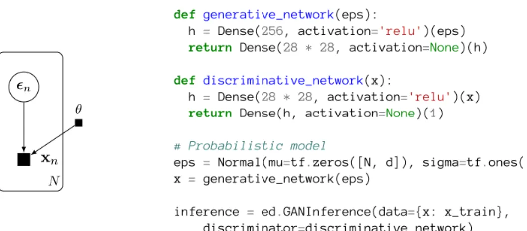
Figure 2.7: Generative adversarial networks:(left)graphical model;(right)probabilistic program. The model (generator) uses a parameterized function (discriminator) for training.
mass concentrated at a point.MAPinherits fromVariationalInferenceand defines the negative log joint density as the loss function; it uses existing optimizers inside TensorFlow. InSection 2.4.1, we experiment with multiple gradient estimators for black box variational inference (Ranganath et al.,2014). Each estimator implements the same loss (an objective proportional to the divergence
KL(qkp)) and a different update rule (stochastic gradient).
Monte Carlo approximates the posterior using samples (Robert and Casella,1999). Monte Carlo is an inference where the approximating family is an empirical distribution,q(β;{β(t)}) = T1 PTt=1δ(β, β(t))
andq(z;{z(t)}) = T1 PTt=1δ(z,z(t)). The parameters areλ={β(t),z(t)}. SeeFigure 2.6(right).
Monte Carlo algorithms proceed by updating one sampleβ(t),z(t) at a time in the empirical ap-proximation. Specific mc samplers determine the update rules: they can use gradients such as in Hamiltonian Monte Carlo (Neal,2011) and graph structure such as in sequential Monte Carlo (Doucet et al.,2001).
Edward also supports non-Bayesian methods such as generative adversarial networks (gans) ( Good-fellow et al.,2014). SeeFigure 2.7. The model posits random noiseepsoverN data points, each withddimensions; this random noise feeds into agenerative_networkfunction, a neural network that outputs real-valued data x. In addition, there is adiscriminative_networkwhich takes data as input and outputs the probability that the data is real (in logit parameterization). We build GANInference; running it optimizes parameters inside the two neural network functions. This approach extends to many advances in gans (e.g.,Denton et al.(2015);Li et al.(2015)).
qbeta = PointMass(params=tf.Variable(tf.zeros([K, D])))
qz = Categorical(logits=tf.Variable(tf.zeros([N, K])))
inference_e = ed.VariationalInference({z: qz}, data={x: x_train, beta: qbeta})
inference_m = ed.MAP({beta: qbeta}, data={x: x_train, z: qz}) ...
for _ in range(10000): inference_e.update()
inference_m.update()
Figure 2.8:Combining inference algorithms to perform variational EM.
Finally, one can design algorithms that would otherwise require tedious algebraic manipulation. With symbolic algebra on nodes of the computational graph, we can uncover conjugacy relationships between random variables. Users can then integrate out variables to automatically derive classical Gibbs (Gelfand and Smith,1990), mean-field updates (Bishop,2006), and exact inference. These algorithms are being currently developed in Edward.
2.3.3 Composing Inferences
Core to Edward’s design is that inference can be written as a collection of separate inference programs. Below we demonstrate variational EM, with an (approximate) E-step over local variables and an M-step over global variables. We instantiate two algorithms, each of which conditions on inferences from the other, and we alternate with one update of each (Neal and Hinton,1993), This extends to many other cases such as exact EM for exponential families, contrastive divergence (Hinton,2002), pseudo-marginal methods (Andrieu and Roberts, 2009), and Gibbs sampling within variational inference (Wang and Blei, 2012;Hoffman and Blei, 2015). We can also write message passing algorithms, which solve a collection of local inference problems (Koller and Friedman,2009). For example, classical message passing uses exact local inference and expectation propagation locally minimizes the Kullback-Leibler divergence, KL(pkq)(Minka,2001).
2.3.4 Data Subsampling
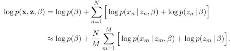
Stochastic optimization (Bottou,2010) scales inference to massive data and is key to algorithms such as stochastic gradient Langevin dynamics (Welling and Teh,2011) and stochastic variational inference (Hoffman et al.,2013). The idea is to cheaply estimate the model’s log joint density in an unbiased way. At each step, one subsamples a data set{xm}of sizeM and then scales densities with
respect to local variables, logp(x,z, β) = logp(β) + N X n=1 h logp(xn|zn, β) + logp(zn|β) i ≈logp(β) + N M M X m=1 h logp(xm|zm, β) + logp(zm|β) i .
To support stochastic optimization, we represent only a subgraph of the full model. This prevents reifying the full model, which can lead to unreasonable memory consumption (Tristan et al.,2014). During initialization, we pass in a dictionary to properly scale the arguments. SeeFigure 2.9.
β
zm xm
M
beta = Normal(mu=tf.zeros([K, D]), sigma=tf.ones([K, D])) z = Categorical(logits=tf.zeros([M, K]))
x = Normal(mu=tf.gather(beta, z), sigma=tf.ones([M, D]))
qbeta = Normal(mu=tf.Variable(tf.zeros([K, D])),
sigma=tf.nn.softplus(tf.Variable(tf.zeros([K, D])))) qz = Categorical(logits=tf.Variable(tf.zeros([M, D])))
inference = ed.VariationalInference({beta: qbeta, z: qz}, data={x: x_batch}) inference.initialize(scale={x: float(N)/M, z: float(N)/M})
Figure 2.9:Data subsampling with a hierarchical model. We define a subgraph of the full model, forming a plate of sizeM rather thanN. We then scale all local random variables byN/M.
Conceptually, the scale argument represents scaling for each random variable’s plate, as if we had seen that random variableN/M as many times. As an example,Appendix A.6shows how to implement stochastic variational inference in Edward. The approach extends naturally to streaming data (Doucet et al.,2000;Broderick et al.,2013;McInerney et al.,2015), dynamic batch sizes, and data structures in which working on a subgraph does not immediately apply (Binder et al.,1997;Johnson and Willsky,
2014;Foti et al.,2014).
2.4 Experiments
In this section, we illustrate two main benefits of Edward: flexibility and efficiency. For the former, we show how it is easy to compare different inference algorithms on the same model. For the latter, we show how it is easy to get significant speedups by exploiting computational graphs.
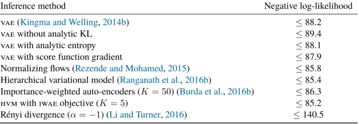
Inference method Negative log-likelihood
vae (Kingma and Welling,2014b) ≤88.2
vae without analytic KL ≤89.4
vae with analytic entropy ≤88.1
vae with score function gradient ≤87.9
Normalizing flows (Rezende and Mohamed,2015) ≤85.8 Hierarchical variational model (Ranganath et al.,2016b) ≤85.4 Importance-weighted auto-encoders (K = 50) (Burda et al.,2016b) ≤86.3
hvm with iwae objective (K= 5) ≤85.2
Rényi divergence (α=−1) (Li and Turner,2016) ≤140.5
Table 2.1: Inference methods for a probabilistic decoder on binarized MNIST. The Edward proba-bilistic programming language (ppl) is a convenient research platform, making it easy to both develop and experiment with many algorithms.
2.4.1 Recent Methods in Variational Inference
We demonstrate Edward’s flexibility for experimenting with complex inference algorithms. We consider the vae setup fromFigure 3.4and the binarized MNIST data set (Salakhutdinov and Murray,
2008). We used= 50latent variables per data point and optimize using ADAM. We study different components of the vae setup using different methods;Appendix A.8is a complete script. After training we evaluate held-out log likelihoods, which are lower bounds on the true value.
Table 4.1shows the results. The first method uses the vae fromFigure 3.4. The next three methods use the same vae but apply different gradient estimators: reparameterization gradient without an analytic KL; reparameterization gradient with an analytic entropy; and the score function gradient (Paisley et al.,2012a;Ranganath et al.,2014). This typically leads to the same optima but at different convergence rates. The score function gradient was slowest. Gradients with an analytic entropy produced difficulties around convergence: we switched to stochastic estimates of the entropy as it approached an optima. We also use hierarchical variational models (hvms) (Ranganath et al.,2016b) with a normalizing flow prior; it produced similar results as a normalizing flow on the latent variable space (Rezende and Mohamed,2015), and better than importance-weighted auto-encoders (iwaes) (Burda et al.,2016b).
We also study novel combinations, such as hvms with the iwae objective, gan-based optimization on the decoder (with pixel intensity-valued data), and Rényi divergence on the decoder. gan-based
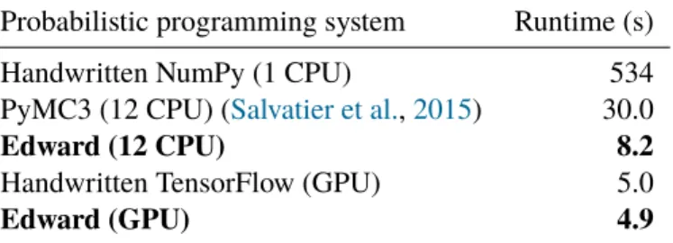
Probabilistic programming system Runtime (s)
Handwritten NumPy (1 CPU) 534
PyMC3 (12 CPU) (Salvatier et al.,2015) 30.0
Edward (12 CPU) 8.2
Handwritten TensorFlow (GPU) 5.0
Edward (GPU) 4.9
Table 2.2: hmc benchmark for large-scale logistic regression. Edward (GPU) is significantly faster than other systems. In addition, Edward has no overhead: it is as fast as handwritten TensorFlow.
optimization does not enable calculation of the log-likelihood; Rényi divergence does not directly optimize for log-likelihood so it does not perform well. The key point is that Edward is a convenient research platform: they are all easy modifications of a given script.
2.4.2 GPU-accelerated Hamiltonian Monte Carlo
β
yn xn
N
# Model
x = tf.Variable(x_data, trainable=False)
beta = Normal(mu=tf.zeros(D), sigma=tf.ones(D))
y = Bernoulli(logits=tf.dot(x, beta))
# Inference
qbeta = Empirical(params=tf.Variable(tf.zeros([T, D]))) inference = ed.HMC({beta: qbeta}, data={y: y_data})
inference.run(step_size=0.5 / N, n_steps=10)
Figure 2.10: Edward program for Bayesian logistic regression with hmc.
We benchmark runtimes for a fixed number of Hamiltonian Monte Carlo (hmc;Neal,2011) iterations on modern hardware: a 12-core Intel i7-5930K CPU at 3.50GHz and an NVIDIA Titan X (Maxwell) GPU. We apply logistic regression on the Covertype dataset (N = 581012,D= 54; responses were binarized) using Edward and PyMC3 (Salvatier et al.,2015). We ran 100 hmc iterations, with 10 leapfrog updates per iteration, a step size of0.5/N, and single precision. Figure 2.10illustrates the program in Edward.
Table 2.2displays the runtimes.Edward (GPU) features a dramatic and 6x speedup over PyMC3 (12 CPU). This showcases the value of building a ppl on top of computational graphs. The speedup stems from fast matrix multiplication when calculating the model’s log-likelihood; GPUs can efficiently parallelize this computation. We expect similar speedups for models whose bottleneck is also matrix multiplication, such as deep neural networks.
PyMC3’s Theano backend compared to Edward’s TensorFlow. Rather, PyMC3 does not use Theano for all its computation, so it experiences communication overhead with NumPy. (PyMC3 was actually slower when using the GPU.) We predict that porting Edward’s design to Theano would feature similar speedups.
In addition to these speedups, we highlight that Edward has no runtime overhead: it is as fast as handwritten TensorFlow. Following Section 2.3.1, this is because the computational graphs for inference are in fact the same for Edward and the handwritten code.
2.5 Discussion
We described Edward, a Turing-complete ppl with compositional representations for probabilistic models and inference. Edward expands the scope of probabilistic programming to be as flexible and computationally efficient as traditional deep learning. For flexibility, we showed how Edward can use a variety of composable inference methods, capture recent advances in variational inference and generative adversarial networks, and finely control the inference algorithms. For efficiency, we showed how Edward leverages computational graphs to achieve fast, parallelizable computation, scales to massive data, and incurs no runtime overhead over handwritten code.
As with any language design, Edward makes tradeoffs in pursuit of its flexibility and speed for research. For example, an open challenge in Edward is to better facilitate programs with complex control flow and recursion. While possible to represent, it is unknown how to enable their flexible inference strategies. In addition, it is open how to expand Edward’s design to dynamic computational graph frameworks—which provide more flexibility in their programming paradigm—but may sacrifice performance. A crucial next step for probabilistic programming is to leverage dynamic computational graphs while maintaining the flexibility and efficiency that Edward offers. We discuss such advances in the next chapter.
Chapter 3: Simple, Distributed, and Accelerated Probabilistic Programming
3.1 Introduction
Many developments in deep learning can be interpreted as blurring the line between model and com-putation. Some have even gone so far as to declare a new paradigm of “differentiable programming,” in which the goal is not merely to train a model but to perform general program synthesis.1 In this view, attention (Bahdanau et al.,2015) and gating (Hochreiter and Schmidhuber,1997) describe boolean logic; skip connections (He et al.,2016) and conditional computation (Bengio et al.,2015;
Graves,2016) describe control flow; and external memory (Giles et al.,1990;Graves et al.,2014) accesses elements outside a function’s internal scope. Learning algorithms are also increasingly dynamic: for example, learning to learn (Hochreiter et al.,2001), neural architecture search (Zoph and Le,2017), and optimization within a layer (Amos and Kolter,2017).
The differentiable programming paradigm encourages modelers to explicitly consider computational expense: one must consider not only a model’s statistical properties (“how well does the model capture the true data distribution?”), but its computational, memory, and bandwidth costs (“how efficiently can it train and make predictions?”). This philosophy allows researchers to engineer deep-learning systems that run at the very edge of what modern hardware makes possible.
By contrast, the probabilistic programming community has tended to draw a hard line between model and computation: first, one specifies a probabilistic model as a program; second, one performs an “inference query” to automatically train the model given data (Spiegelhalter et al.,1995;Pfeffer,2007;
Carpenter et al.,2016). This design choice makes it difficult to implement probabilistic models at truly large scales, where training multi-billion parameter models requires splitting model computation across accelerators and scheduling communication (Shazeer et al.,2017). Recent advances such as
1
Recent advocates of this trend include Tom Dietterich (https://twitter.com/tdietterich/
status/948811925038669824) and Yann LeCun (https://www.facebook.com/yann.lecun/posts/