Volume 39
Article 7
7-2016
Text Mining For Information Systems Researchers:
An Annotated Topic Modeling Tutorial
Stefan Debortoli
University of Liechtenstein, [email protected]
Oliver Müller
IT University of Copenhagen
Iris Junglas
Florida State University
Jan vom Brocke
University of LiechtensteinFollow this and additional works at:
http://aisel.aisnet.org/cais
This material is brought to you by the Journals at AIS Electronic Library (AISeL). It has been accepted for inclusion in Communications of the Association for Information Systems by an authorized administrator of AIS Electronic Library (AISeL). For more information, please contact
Recommended Citation
Debortoli, Stefan; Müller, Oliver; Junglas, Iris; and vom Brocke, Jan (2016) "Text Mining For Information Systems Researchers: An Annotated Topic Modeling Tutorial,"Communications of the Association for Information Systems: Vol. 39 , Article 7.
DOI: 10.17705/1CAIS.03907
C
A
I
S
ssociation
for
nformation
ystems
Tutorial ISSN: 1529-3181
Volume 39 Paper 7 pp. 110 – 135 July 2016
Text Mining For Information Systems Researchers: An
Annotated Topic Modeling Tutorial
Stefan Debortoli University of Liechtenstein Institute of Information Systems
Vaduz, Liechtenstein
Oliver Müller
IT University of Copenhagen Information Management Section
Copenhagen, Denmark
Iris Junglas Florida State University
College of Business Tallahassee, FL, USA
Jan vom Brocke University of Liechtenstein Institute of Information Systems
Vaduz, Liechtenstein
Abstract:
Analysts have estimated that more than 80 percent of today’s data is stored in unstructured form (e.g., text, audio, image, video)—much of it expressed in rich and ambiguous natural language. Traditionally, to analyze natural language, one has used qualitative data-analysis approaches, such as manual coding. Yet, the size of text data sets obtained from the Internet makes manual analysis virtually impossible. In this tutorial, we discuss the challenges encountered when applying automated text-mining techniques in information systems research. In particular, we showcase how to use probabilistic topic modeling via Latent Dirichlet allocation, an unsupervised text-mining technique, with a LASSO multinomial logistic regression to explain user satisfaction with an IT artifact by automatically analyzing more than 12,000 online customer reviews. For fellow information systems researchers, this tutorial provides guidance for conducting text-mining studies on their own and for evaluating the quality of others.
Keywords: Text Mining, Topic Modeling, Latent Dirichlet Allocation, Online Customer Reviews, User Satisfaction.
This manuscript underwent editorial review. It was received 05/26/2015 and was with the authors for 8 months for 3 revisions. The Associate Editor chose to remain anonymous.
Volume 39 Paper 7
1
Introduction
With the emergence of the Web 2.0 and social media, the amount of unstructured, textual data on the Internet has grown tremendously, especially at the micro level (Gopal, Marsden, & Vanthienen, 2011). For example, at the time of writing, Amazon.com alone offered more than 140 million customer reviews about more than nine million products that millions of Amazon users have written over almost 20 years (McAuley, Pandey, & Leskovec, 2015; McAuley, Targett, Shi, & van den Hengel, 2015). And the over 300 million active Twitter users have generated an average of 500 million Tweets per day (Twitter, 2015). This abundance of publicly available data creates new opportunities for both qualitative and quantitative information systems (IS) researchers.
Traditionally, to analyze natural language data, one has used qualitative data-analysis approaches, such as manual coding (Quinn, Monroe, Colaresi, Crespin, & Radev, 2010). Yet, the size of textual data sets available from the Internet exceeds the information-processing capacities of single researchers and even research teams. And despite methodological guidelines on how to improve the validity and reliability when analyzing qualitative data with multiple coders (Saldaña, 2012), one cannot completely mitigate the biases arising from researchers’ subjective interpretations of the data (Indulska, Hovorka, & Recker, 2012). Text-mining techniques allow one to automatically extract implicit, previously unknown, and potentially useful knowledge from large amounts of unstructured textual data in a scalable and repeatable way (Fan, Wallace, Rich, & Zhang, 2006; Frawley, Piatetsky-Shapiro, & Matheus, 1992). Although the automated computational analysis of text only scratches the surface of a natural language’s semantics, it has proven to be a reliable tool when fed with sufficiently large data sets (Halevy, Norvig, & Pereira, 2009). Against this background, text mining offers an interesting and complimentary strategy of inquiry for IS research that one can combine with other data-analysis methods (e.g., regression analysis) or use to triangulate research results gained from more traditional data-collection and analysis methods. In particular, automated text mining allows IS researchers to 1) overcome the limitations of manual approaches to analyzing qualitative data and 2) yield insights that they could not otherwise find. The following two examples illustrate these points.
In a study that has received much public and scholarly attention, Michel et al. (2011) investigated cultural trends by computing the yearly relative frequency of words appearing in Google Books. This simple statistical analysis, applied to more than five million digitized books, produced some interesting insights. The study found, for instance, that the diffusion of innovations, measured by word frequencies corresponding to certain technologies (e.g., radio, telephone) over time, has accelerated at an increasing rate. While at the beginning of the 19th century it took an average of 66 years from invention to the widespread adoption of a technology, the average time to adoption dropped to 27 years around 1900. Another illustrative example comes from social psychology. Pennebaker (2011) and Tausczik and Pennebaker (2010) developed the Linguistic Inquiry and Word Count (LIWC) tool that allows one to automatically quantify the linguistic style of texts by counting different function words (e.g., pronouns, articles, prepositions). Function words occur frequently in natural language, but readers—and coders— usually do not consciously pay attention to them and focus on content words (e.g., nouns, verbs) instead. Yet, researchers found that subtle differences in usage patterns of function words are important predictors for numerous psychological states. Researchers have used LIWC, for instance, to detect deception in online customer reviews: reviewers who lie tend to use more personal pronouns and “I” words and less concrete terms (e.g., numbers) than truthful reviewers (Ott, Choi, Cardie, & Hancock, 2011).
In this tutorial, we discuss the challenges encountered when applying automated text-mining techniques in IS research. Applying text mining requires the skill sets of a diverse set of fields, including computer science and linguistics, and not every IS researcher is familiar with these fields’ concepts and methods. While much technical literature on the ideas and methods underlying specific text-mining algorithms exists, such as topic modeling (Blei, 2012) or sentiment analysis (Pang & Lee, 2008), these publications rarely touch on the “how-to” aspects of applying text mining as a strategy of inquiry for (information systems) research. We particularly focus on probabilistic topic modeling as a technique for inductively discovering topics running through a large collection of texts (corpus), such as user-generated content from the Web. In addition to outlining the foundations of topic modeling, we illustrate its concrete use by presenting available software tools and showcasing their application with the help of an integrated example from the area of online customer reviews.
Volume 39 Paper 7
This paper proceeds as follows. In Section 2, we overview approaches for analyzing large text corpora in general and delve into probabilistic topic modeling in particular. In Section 3, we discuss typical challenges encountered in topic modeling studies and outline potential ways for overcoming them. In Section 4, we introduce tools for applying topic modeling and illustrate their application with the help of an integrated example. In Section 5, we conclude by discussing the limitations of the presented methods.
2
Background
2.1
Analyzing Large Text Corpora
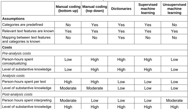
One of the most fundamental tasks in analyzing text (both manually and automatically) is categorizing text; that is, assigning chunks of texts (e.g., emails, social media comments, news) to one or more categories (e.g., spam or no spam, positive or negative sentiment, business or politics or sports news). One can use different methods to categorize text, and each of them is associated with certain assumptions and costs (see Table 1).
Traditionally, researchers have manually coded text to categorize it (Berg & Lune, 2011). In coding, one differentiates and combines data into categories to capture its essential meaning (Miles & Huberman, 1994). Various coding techniques exist (see, e.g., Saldaña, 2012); however, at the most basic level, one can distinguish between bottom-up and top-down approaches (Urquhart, 2012). As part of bottom-up coding, the data suggests the codes (i.e., words and phrases) regardless of extant theory (Urquhart, 2012). The coder should analyze the data with an open mind and not impose preconceptions on it. In contrast, for top-down coding, coders use a predefined coding schema derived from literature and assign the data to these codes (Urquhart, 2012). Researchers sometimes use this latter style of coding in combination with counting instances of codes (e.g., when doing systematic content analysis).
Manual coding has many strengths, such as individuals’ unrivaled capacity to understand the meaning of natural language or the possibility for highly complex and contingent mappings between text features and categories (Quinn et al., 2010). Yet, it also suffers from several limitations. First, it is prone to human subjectivity, and, hence, different coders may end up with different results (Urquhart, 2001). To overcome these threats to validity and reliability, researchers have proposed various strategies for achieving intersubjective verifiability, such as using codebooks, having multiple coders, or conducting inter-coder reliability tests (Indulska et al., 2012). Yet, a second limitation of manual coding limits the applicability of these strategies: manual coding is costly in terms of needed person hours and requires substantive domain knowledge (Quinn et al., 2010). To overcome these limitations, researchers have developed computer-aided approaches for analyzing text by applying dictionary-based or machine-learning algorithms.
A dictionary-based text categorization relies on experts assembling lists of words and phrases that likely indicate text’s membership to a particular category (Quinn et al., 2010). Using this dictionary, a computer can then automatically parse through large amounts of text and determine the classification of a unit of text. One can only use a dictionary-based categorization if one predefines categories and one knows and can codify the mapping between text features (i.e., words and phrases) and categories in advance. In other words, one can only apply dictionary-based approaches to automate top-down manual coding. Many sentiment analysis methods, which classify texts into positive or negative categories, such as the popular SentiStrength (Thelwall, Buckley, Paltoglou, Cai, & Kappas, 2010), use dictionary-based text categorization methods.
A second approach of automating top-down manual coding involves using supervised learning methods. Like before, one knows and has predefined categories; however, one does not explicitly know the mapping between text features and categories (Quinn et al., 2010). Using a set of manually classified documents as training examples, one can then apply supervised machine-learning algorithms to automatically detect a relationship between the usage of a word and its category assignments. One can then use the learned patterns to classify new or unseen texts. Email spam filtering is a classic example of effectively using supervised learning methods to categorize text by, for example, picking out words that frequently appear in advertisements such as “$$$”, “credit”, and “free”.
Finally, unsupervised machine-learning methods for categorizing text find hidden structures in texts for which no predefined categorization exists (Quinn et al., 2010). Unsupervised learning methods (e.g., clustering, dimensionality reduction) use features of texts to inductively discover latent categories and assign units of texts to those categories. This inductive approach is comparable to manual bottom-up
Volume 39 Paper 7
coding or open coding as known from the grounded theory method (Berente & Seidel, 2014). Unsupervised text-categorization approaches have some distinct advantages over manual coding: 1) they require only little human intervention and substantive knowledge in the pre-analysis and analysis phases, 2) they generate reproducible results since they are not subject to the human subjectivity bias, and 3) today’s algorithms and computing systems can cope with ample volumes of texts that would be impossible to analyze even with large coding teams. On the downside, unsupervised methods require an extensive post-analysis phase that is typically time consuming because a researcher has to make sense of the automatically generated inductive categorizations.
Table 1. Assumptions and Costs of Different Text-categorization Methods (Adapted and Extended from Quinn et al., 2010)
Manual coding (bottom up)
Manual coding
(top down) Dictionaries
Supervised machine learning Unsupervised machine learning Assumptions
Categories are predefined No Yes Yes Yes No
Relevant text features are known Yes Yes Yes Yes Yes
Mapping between text features
and categories is known No No Yes No No
Costs
Pre-analysis costs
Person-hours spent
conceptualizing Low High High High Low
Level of substantive knowledge Low High High High Low
Analysis costs
Person-hours spent per text High High Low Low Low
Level of substantive knowledge Moderate Moderate Low Low Low
Post-analysis costs
Person hours spent interpreting Moderate Low Low Low Moderate
Level of substantive knowledge High High High High High
2.2
Probabilistic Topic Modeling
In this section, we discuss probabilistic topic modeling, an unsupervised machine-learning method, in more detail. Unsupervised machine-learning methods rely only on few assumptions in terms of the underlying text data and require minimal costs for analyzing data; hence, researchers can apply them on a broad variety of sources and large volumes of data.
The underlying idea of many unsupervised learning methods for categorizing text is rooted in the distributional hypothesis of linguistics (Firth, 1957; Harris, 1954), which refers to the observation that “words that occur in the same contexts tend to have similar meanings” (Turney & Pantel, 2010, p. 142). For example, one could interpret co-occurring words such as “goal”, “ball”, “striker”, and “foul” in newspaper articles as markers for a common category (namely “football”) and use them to group articles accordingly.
Researchers have developed and extended several distributional methods for unsupervised text categorization over the last several decades. Among the most frequently used approaches in IS research are latent semantic analysis (Landauer, Foltz, & Laham, 1998), latent Dirichlet allocation (Blei, Ng, & Jordan, 2003) and Leximancer (Smith & Humphreys, 2006). Latent semantic analysis (LSA) extracts distributional word-usage patterns through reducing the dimensionality of a term-document matrix by applying a singular value decomposition. Researchers often interpret the resulting latent semantic factors, which share many similarities with the outputs of factor analysis or principal components analysis, as topics (Landauer et al., 1998). LSA has been a groundbreaking development in the computational linguistics field, but it suffers from interpretability issues because the computed factor loadings often have no clear interpretation. To overcome these shortcomings, researchers have developed probabilistic LSA
Volume 39 Paper 7
(pLSA) (Hofmann, 1999) and latent Dirichlet allocation (LDA) (Blei et al., 2003; Blei, 2012) as extensions to the classic LSA idea. In both methods, the associations between documents and topics and between topics and words are represented as probability distributions that one can use for further statistical analyses. For example, one can group and aggregate the estimated probability distributions by document metadata or use them as predictors in regression or classification models. Also, various commercial tools exist that are based on the distributional hypothesis. Leximancer (http://www.leximancer.com), for example, combines unsupervised extraction of word co-occurrence patterns with concept mapping and intuitive visualizations (Smith & Humphreys, 2006). However, Leximancer’s algorithms and data structures are patented and, hence, only scarcely documented.
In the following paragraphs, we describe the application of probabilistic topic modeling with LDA in detail. We chose LDA for three reasons: 1) LDA has evolved from the seminal LSA idea, and academic research has extensively used both methods1; 2) numerous free and open source LDA software libraries exist for
most statistical programming languages (including R, Python, Java); and 3) several empirical studies have validated LDA’s capability of extracting semantically meaningful topics from texts and categorizing texts according to these topics (e.g., Boyd-Graber, Mimno, & Newman, 2014; Chang, Boyd-Graber, Gerrish, Wang, & Blei, 2009; Lau, Newman, & Baldwin, 2014; Mimno, Wallach, Talley, Leenders, & McCallum, 2011).
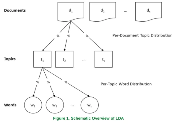
The core idea behind LDA, first proposed by Blei et al. (2003), is an imaginary generative process that assumes that authors compose d documents by choosing a discrete distribution of t topics to write about
and drawing w words from a discrete distribution of words that are typical for each topic (see Figure 1). In
other words, a probability distribution over a fixed set of topics defines each document, and, in turn, a probability distribution over a confined vocabulary of words defines each topic. While LDA assumes all documents to be generated from the same fixed set of topics, each document exhibits these topics in different proportions that can range from 0 percent (if a document fails to talk about a topic entirely) to 100 percent (if a document talks about a topic exclusively). The LDA algorithm computationally estimates the hidden topic and word distributions given the observed per-document word occurrences. LDA can perform this estimation via sampling approaches (e.g., Gibbs sampling) or optimization approaches (e.g., Variational Bayes).
Figure 1. Schematic Overview of LDA
1 At the time of writing, a search on Google Scholar for “latent semantic analysis“ produced over 32,000 hits, and a search for “latent
Volume 39 Paper 7
Figure 2 illustrates the basic idea behind LDA using an exemplary online customer review about a “Fitbit Flex” 2 device and its topic distribution and six topics and their word distributions. The exemplary review
covers three topics to different degrees; namely, topic 3 (55%), topic 2 (35%), and topic 6 (10%); other topics are not present (0%). In turn, a distribution over words represents each topic. Topic 3, for example, assigns high likelihood for words such as “weight” (8%), “loss” (5%), and “pounds” (4%), which indicates that the topic covers weight loss as an effect of using the Fitbit device. Topic 2, on the other hand, has highly probable words such as “gift” (10%), “love” (7%), or “Christmas” (7%), which indicates that the Fitbit device has been given or received as a present. Finally, the most probable words for topic 6 are “app” (12%), “iPhone” (8%), and “sync” (3%), which refer to the synchronization between the Fitbit and the corresponding iPhone app.
Figure 2. Illustrative Example of LDA
3
Practical Challenges of Applying Topic Modeling
We now turn to the practical challenges one faces when applying topic modeling as a method for automated analysis of large sets of qualitative data. These challenges roughly mirror the phase of a typical research process.
3.1
Challenge #1: Obtaining Data from the Web
As topic modeling produces valid results only when fed with a sufficiently large data set (n > 1,000), researchers do not typically use it for analyzing data they have collected themselves (e.g., interview transcripts, field notes) but for analyzing texts that a large group of people have produced (e.g., user-generated content originating from social media websites; research papers written by a scientific community) and are available as Internet resources. In broad terms, one can extract text data from Internet sources in three ways: 1) via Application Programming Interfaces (APIs), 2) via Web crawlers, or 3) via file downloads.
APIs are programmatic data access points that data providers make available to offer reusable content in a controlled way (e.g., by restricting the scope and amount of data that can be accessed) and in a structured format (e.g., by using markup languages such as XML or JSON). While extracting data via APIs usually ensures high levels of data quality, providers will only rarely expose the full breadth and depth of their data via APIs—in the best of cases, they require users to pay for such data requests. A popular API used in text mining studies is the Twitter API because it is subject to few restrictions. While the APIs to social networks such as Facebook, LinkedIn, or Google+ only permit access to data about “friends”, the Twitter API provides access to data about all members of the network.
Volume 39 Paper 7
Web crawlers offer another way to extract data from the Web. These automated programs traverse the Web’s topology and download relevant pages and hyperlinks (Liu, 2011). Data consumers or intermediaries rather than data providers operate them. Web crawlers parse, or “scrape”, a webpage’s content using simple natural language processing heuristics (e.g., regular expressions). Because webpages typically contain lots of noise (e.g., HTML tags, advertisement banners), many Web crawlers try to filter out irrelevant elements—with more or less success. In addition to extracting content, Web crawlers can capture the Web’s underlying linkages and social structures by building a graph of interconnected actors (e.g., webpages, users). Overall, Web crawlers provide researchers with lots of flexibility. For example, a researcher can develop a crawler that targets specific topics by initializing it with a set of search terms or seed URLs. Such flexibility, however, comes at a price. Crawlers often require in-depth programming, and the quality of data they gather might not be up to par to what one requires for analysis.
Finally, researchers can also use open data sets that they can download from the Web. Open data comprises data that anyone can freely use, reuse, and redistribute; individuals are subject only to the requirement of attribution (OKF, 2012). Over the last several years, governments (e.g., http://www.data.gov/), not-for-profit organizations (e.g., http://en.wikipedia.org/wiki/ Wikipedia:Database_download), research institutions (e.g., https://snap.stanford.edu/data/), and private organizations (e.g., http://www.yelp.com/dataset_challenge) have established open data repositories that contain large collections of text data that can be of interest to IS researchers. Most of these data sets are integrated and curated, which eases access and ensures data quality.
In choosing a data-collection approach, researchers also have to consider the period they can capture. Data snapshots are the easiest to accomplish and are supported by most APIs and Web crawlers. Also, many open data sets come from cross-sectional surveys and, hence, represent snapshots. Collecting longitudinal data are more problematic. While some APIs and open data sets provide historical data, Web crawling is done in periodic batch runs that cannot capture the full volatility of webpages. Finally, the most difficult time frame to capture is data in real time. Only so-called streaming APIs, such as Twitter’s Firehose API that allows real-time access to the complete stream of Tweets (currently about 4,000 Tweets per second), can provide this capability. However, only selected partner organizations can access Firehose.
3.2
Challenge #2: Readying Data for Analysis
A lack of well-defined structures and a high proportion of noise characterize natural language data. Hence, in almost all cases, the data needs to undergo an extensive preprocessing phase before one can statistically analyze it through topic models. Although one rarely highlights the data-preparation steps when presenting the research results, they typically require 45 to 60 percent of the overall effort (Kurgan & Musilek, 2006).
As a first step, one should perform a high-level exploratory data analysis (EDA) to obtain an initial feeling for the data set and to identify potential data quality problems. Besides computing summary statistics (e.g., number of documents in the data set, average number of words per document), researchers should use visualizations. For example, word-frequency plots provide valuable information about required data cleaning and natural language-processing steps. Likewise, plotting timestamps of documents on a timeline can quickly reveal missing data (and, thus, potentially point to errors during data collection) or temporal trends and seasonal patterns. If the obtained text documents contain numerical information that one plans to use in later analyses (e.g., as independent or dependent variables in a regression analysis), one should also plot them to visualize their distributions and identify potential anomalies.
After having explored the overall data set, one needs to inspect and preprocess the obtained texts at the document level. Typical preparation steps include: data cleaning, data construction, data formatting, and natural language processing.
Data cleaning is one of the fundamental steps in readying natural language data for analysis by removing duplicates and noise. Because many data sets used in text mining studies constitute secondary data, the chance that they contain “unclean” data is rather high. For example, posts on online social networks such as Twitter might contain duplicate records (retweets, spam), and data collected by Web crawlers might contain noise in the form of HTML tags. Duplicates and noise, if left unattended, may lead to not only biased but also incorrect results.
Volume 39 Paper 7
Data construction entails deriving new attributes and/or records. Examples of derived attributes include computations involving multiple attributes (e.g., calculating the longevity of an online review by subtracting the date of creation from the current date) or single attribute transformations (e.g., tagging reviews with geographic locations). Whether one needs to create new data attributes highly depends on the subsequent data-analysis procedure. To ensure transparency, researchers should provide exact formulas for how they derived new attributed.
After these initial steps, one needs to (re-)format the data set in order to bring it into a format that is appropriate for statistical analysis. Re-formatting can range from simple changes of individual values (e.g., removing illegal characters or changing character encodings) to complex data model transformations. For example, data extracted via APIs, Web crawlers, or downloads are mostly represented in flat files (e.g., CSV) or hierarchical data models (e.g., XML, JSON); for analysis and storage, one might find it useful to convert such data into a relational (e.g., for SQL databases) or key-value data model (e.g., for NoSQL databases). Ideally, one illustrates and sufficiently documents the original data model with its various sources and the final data model used for analytical purposes.
After document-level preprocessing, the set of individual documents undergoes several low-level natural-language processing (NLP) steps, such as tokenization (i.e., splitting up documents into sentences and sentences into words), n-gram creation (i.e., creating n consecutive words: 1-grams include, for example, “fast”, “food”, or “chain”; 2-grams concatenate two 1-grams, such as “fast food”; and 3-grams comprise three 1-grams, such as “fast food chain”), stopping (i.e., removing common or uninformative words), part-of-speech filtering (i.e., identifying and filtering words by their part of speech), lemmatizing (i.e., reducing a word into its dictionary form; for example, plural to singular for nouns, verbs to the simple present tense), stemming (i.e., reducing a word to its stem), and the creation of a structured numerical representation of the document collection (e.g., creating a vector or matrix representation) (Miner et al., 2012). The common objective of these transformations is to remove noise and to gradually turn qualitative textual data into a numerical representation that is amenable to latter statistical analysis. Unfortunately, we have no easy recipe for selecting the appropriate combination of natural language preprocessing steps. A study’s goal and its underlying dataset determine many of the steps. However, one can apply some strategies in terms of stop-word removal, text normalization, and collocation discovery (Boyd-Graber et al., 2014) that alleviate the dilemma to some extent.
To identify stop words, generating word frequency lists (i.e., counts of the number of occurrences of every word in a text corpus) is a useful approach. For example, when studying online customer reviews about the Apple iPhone, the terms “Apple” and “iPhone” will have high frequency counts but do not add particular value to the analysis and, therefore, may be removed. One can also apply other approaches, such as term frequency-inverse document frequency (TF-IDF) weighting of word counts to automatically filter uninformative terms (Salton & McGill, 1983).
Text normalization typically includes converting all characters to lower-case and lemmatizing every word. For example, the words “dog”, “Dog”, “dogs”, and “Dogs” would all change to “dog”. One can even push the concept of text normalization further by applying stemming. For example, stemming would reduce the words “analyze” and “analysis” to “analy”. This reduction, however, might lead to another problem (Evangelopoulos, Zhang, & Prybutok, 2012); namely, that one will not be able to differentiate whether “analy” refers to a noun or verb in a given context.
Finally, one can discover collocations of words, or multi-word expressions (i.e., n-grams | n > 1), to help find the correct meaning of words. For example, the word “house” means one thing in a given context, but the word “white house” has, in the majority of cases, an entirely different meaning. Therefore, we recommend performing an n-gram analysis with n > 1, particularly where humans will later interpret the results.
3.3
Challenge #3: Fitting and Validating a Topic Model
Fitting a topic model to a collection of documents can be challenging. The LDA algorithm is sensitive to changes in its parameters and variations in input data introduced, for example, through different data preparation procedures.
The most crucial LDA parameter is the number of topics one plans to extract (Blei et al., 2003; Boyd-Graber et al., 2014). When choosing too many topics, the algorithm might unearth a plethora of only minimally distinct topics (e.g., topics differ in writing style but not in content), and choosing too few topics might unnecessarily constrain the exploratory potential of topic modeling. Therefore, one should vary the
Volume 39 Paper 7
number of topics and to evaluate the quality of the resulting models based on the study’s goals. If one seeks to create a topic model that humans can interpret, then one would typically choose a low number of topics (e.g., between 10 and 50). If, in contrast, one seeks the topic model to serve as input for another statistical model (e.g., regression, classification, clustering) and human comprehensibility is not an important factor, the model fit (and not its interpretability) determine the most appropriate number of topics; here, the number of topics might range between 30 and 100 or even more.
Other parameters that one has to choose as part of the LDA setup include the hyperparameters α and β, which control the shape of the per-document topic distribution and per-topic word distribution, respectively. A large α leads to broad topic distributions (i.e., documents contain many topics), and a large
β leads to broad word distributions (i.e., topics contain many words). In contrast, small values for α and β
lead to more sparse distributions (i.e., documents contain only few topics and topics contain only few words). Although many topic modeling tools allow users to define α and β explicitly, researchers commonly use established standard values (e.g., one divided by the number of topics) or rely on optimization techniques (see Wallach, Mimno, & McCallum, 2009) to automatically determine appropriate values.
Once one has calculated the topic model, one has to interpret the results. For presentation purposes, researchers often display the LDA results in form of lists that show the top-n most likely words per topic (Ramage, Rosen, Chuang, Manning, & McFarland, 2009). While intuitive, this presentation style can bias the investigator because each topic is actually a distribution over the full vocabulary found in the corpus. Therefore, when interpreting the meaning of a topic, we advise a researcher to inspect the actual word probabilities (and not only their rankings) and the documents strongly associated with each topic (which one can obtain through the per-document topic distribution). Often, researchers then assign descriptive labels to topics to assist readers in interpreting topics. As with manually coding texts, at least two independent researchers should interpret and label the topics.
Validating topic models can be difficult. Due to its unsupervised nature, we have no ground truth or gold standard with which to compare the topic modeling outputs. Therefore, in the computer science community, researchers often evaluate topic models by either measuring their performance for a subsequent task (e.g., information retrieval, regression, classification), or by measuring how well a model trained on a given corpus fits an unseen, or held-out, text (for an overview, see Wallach, Murray, Salakhutdinov, & Mimno, 2009). Both approaches assume that another algorithm uses the topic model. Yet, experiments have shown that topic models with high predictive accuracy do not necessarily possess good human interpretability (Chang et al., 2009).
For topic models intended for humans to interpret, Boyd-Graber et al. (2014) propose two guiding questions to evaluate their semantic qualities:
1. Are individual topics meaningful, interpretable, coherent, and useful?
2. Are assignments of topics to documents meaningful, appropriate, and useful?
Common threats to the interpretability of individual topics (question 1) are multi-fold (Boyd-Graber et al., 2014). Too many common words—or, alternatively, too many specific words (e.g., names, numbers)—that either cause topics to be too broad or too specific can prevent a researcher from gaining a deeper understanding of the topic. Adjusting the list of stop words and re-running the analysis might help to resolve these issues.
Another reason for low-quality topics are so-called mixed topics. While the words do not make sense when taken together, they contain subsets of words, which—when taken together—make perfect sense. In other words, mixed topics contain more than one topic and should be split. The opposite is true for identical topics where the algorithm proposes two topics that are semantically equivalent. One can avoid both mixed and identical topics by either increasing or decreasing the number of topics one plans to extract.
Finally, one may always encounter a nonsensical topic. Such a topic can occur, for example, if the documents exhibit a particular structural pattern and/or have a common writing style and vocabulary. For example, a set of research papers that frequently contain the words “figure” and “table” might cause an algorithm to generate a topic based on those words. While adding these words to the algorithm’s stoplist seems a viable option, it would most likely compromise the quality of other topics. Hence, excluding the topics from further analysis is typically the best solution.
Volume 39 Paper 7
Only recently, researchers have started to develop some quantitative criteria to evaluate the semantic quality of individual topics by comparing the algorithm’s word assignments with that of human users (Ramage et al., 2009) or by measuring the statistical properties of topics (Boyd-Graber et al., 2014). For instance, the word intrusion task (see Chang et al., 2009) quantifies the semantic coherence of topics. In this task, one presents six randomly ordered words to human evaluators. One draws five words from the most probable words of a given topic and one word—the intruder—randomly from the vocabulary of the corpus. The idea is that, for a topic to be semantically coherent, a human judge should be able to easily spot the intruder. For example, most people would identify the word “apple” as the intruder in the topic defined by the words “dog”, “cat”, “horse”, “apple”, “pig”, and “cow” (Boyd-Graber et al., 2014). In contrast, one would find it difficult to identify the word “coffee” as the intruder in the following topic defined by the semantically incoherent words “table”, “sky”, “apple”, “yellow”, “city”, and “coffee”.
Instead of humans, one can also use automated approaches to measure topic coherence (Lau et al., 2014; Mimno et al., 2011; Newman, Lau, Grieser, & Baldwin, 2010). Most automated approaches compare the most frequently used words of a topic with texts known to have a high semantic coherence, such as Wikipedia or newspaper articles. The idea is that words of highly coherent topics (e.g., dog, cat, horse, apple, pig, cow) should frequently co-occur in a reference text (e.g., a Wikipedia article about animals); if they do not, the topic has low semantic coherence.
One can apply a similar logic to validate the assignments of topics to documents (question 2). Using a topic intrusion task in which one presents a random document to human evaluators by offering four topic choices, each represented by its top-n most likely words, one can assess the validity of topic-to-document assignments. Three of the topics exhibit a high likelihood for being associated with the document under question, and one topic is random (Chang et al., 2009). Measuring how well human coders can identify the intruder topic indicates the quality of the document-topic assignments made by the LDA algorithm.
3.4
Challenge #4: Going Beyond Description
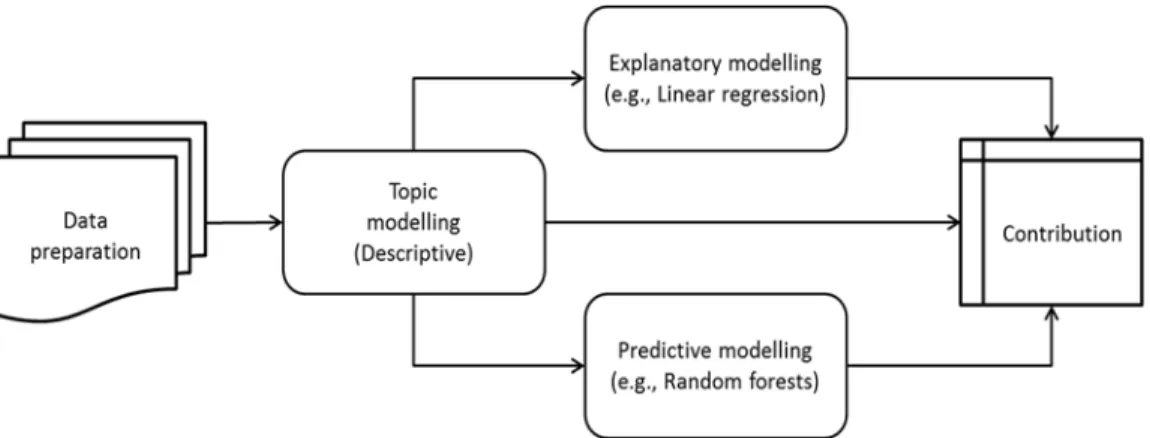
Topic models are, by default, descriptive in nature (i.e., they represent quantitative summaries of large document collections). Descriptive models are sometimes a study’s (exploratory studies in particular) main objective (e.g., the competency taxonomy that Debortoli et al. (2014) derived from job advertisements). Because topic models represent all associations as probabilities, a researcher can not only present relevant topics along with selected word and document distributions but also group and aggregate topic probabilities by different document meta data (e.g., by author, geography, time), which allows one to rank topics by prevalence, to compare their prevalence for specific subgroups, or to track the evolution of topics over time (for examples, see Grimmer & Stewart, 2013).
Apart from descriptive purposes, one can also use topic models for explanatory or predictive purposes (Blei et al., 2003). For that, one uses the estimated per-document topic probabilities as independent variables or predictors in a regression or classification model. Müller, Junglas, vom Brocke, and Debortoli (2016), for example, use the probabilistic topic assignments of more than one million online customer reviews about video games to build a statistical model that can predict the helpfulness of a new or unseen review.
Volume 39 Paper 7
As we mention above, a study’s objective (i.e., description, explanation, prediction) has important implications for topic model fitting. Researchers that focus on describing or on feeding a topic model into a subsequent explanatory model to test hypotheses tend to apply more granular topic models (e.g., 10-50 topics) so they can present their results in full length and in a comprehensible way. In contrast, when a study focuses on prediction—and the comprehensibility of the results are less important—research has shown that more high-dimensional representations of documents (e.g., 100+ topics) in combination with non-linear regression or classification techniques (e.g., highly accurate but otherwise “black box” random forests models) produce the most accurate results. Yet, humans find it difficult—if not impossible—to understand these models and techniques. As a result, they are less useful for description and explanation purposes (see, e.g., Martens and Provost (2014) for a more detailed discussion).
Finally, one needs to engage with existing theories and literature to do more than simply describe a given corpus. For example, one can map the automatically identified topics with known theoretical constructs to place them in their nomological network. Similar to the topic-labeling approach, multiple researchers should engage in this topic-construct mapping task. To do so, one needs to deeply understand the domain of interest and its theoretical foundation to draw valid conclusions. One may also find it useful to provide a list of definitions of the theoretical constructs that all participating coders will likely discover to establish a common understanding. In case a topic does not correspond to an existing construct, a researcher may want to theorize about its ontology.
4
An Illustrative Topic Modeling Study
In this section, we illustrate the practical application of topic modeling in combination with explanatory regression analysis using online customer reviews as an exemplary data source. We structure how we present the illustrative example loosely according to the cross-industry process for data mining (CRISP-DM) framework, which comprises the phases business understanding (which we renamed into research question), data understanding, data preparation, modeling, evaluation, and deployment (which we renamed into interpretation) (Shearer, 2000).
4.1
Research Question
With our illustrate text mining study, we explain users’ satisfaction with a consumer electronics product (as defined by its star rating) by mining the textual and unstructured parts of reviews. Our intuition that the appearance of certain topics in online customer reviews has a significant impact on the corresponding star rating drove our approach. As an exemplary product, we chosen the “Fitbit Flex Wireless Activity & Sleep Wristband” (https://www.fitbit.com/flex), one of the early wearable technologies to track and analyze individuals’ personal health and fitness data around the clock.
4.2
Data Understanding
Online customer reviews are “peer-generated product evaluations posted on company or third party web-sites” (Mudambi & Schuff, 2010). Besides freeform text comments, reviews typically contain a numerical product rating (often on a scale from 1 to 5 stars) and additional metadata (e.g., reviewer name, date of review, helpfulness votes). Amazon, the largest Internet-based retailer in the world, is also one of the largest sources of online customer reviews (Business Wire, 2010). For the “Fitbit Flex” device, Amazon provides more than 12,900 customer reviews (as of May 2015).
Since most e-commerce platforms do not offer APIs to access customer reviews, one often needs to collect reviews via Web crawling. For this tutorial, we developed a Web crawler that captured all historical product reviews of the “Fitbit Flex” on Amazon. We used the Python package “Beautiful Soup” (http://www.crummy.com/software/BeautifulSoup/), which is designed for extracting data out of HTML files. After downloading the reviews from Amazon, we formatted them as a list of JavaScript object notation (JSON) objects to be compatible with the text-mining tool we used for topic modeling. Figure 4 shows an exemplary customer review in JSON format. Besides the textual comments, it contains additional metadata, such as the star rating (between 1 and 5), the author (anonymized), and the review date. In total, we crawled 12,910 reviews from between March 2012 and May 2015.
Volume 39 Paper 7 Figure 4. Example of an Online Customer Review in JSON Format
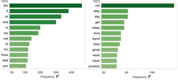
Next, we performed an exploratory data analysis. Calculating and plotting descriptive statistics, such as the number of reviews (12,910), number of words (457,239), number of unique words (4,556) and overall word frequencies, provided a first overview of the data set. For instance, an initial word frequency plot showed (Figure 5) that function words such as articles and pronouns dominated the corpus. Because these words bear little meaning, we decided to remove them in the subsequent data-preparation phase.
Figure 5. Word-frequency Plots Before (left) and After (right) Data Preparation
Because each customer review had metadata, we could plot the distribution of reviews along a temporal dimension (Figure 6). Interestingly, we observed that the number of reviews spiked in the last week of December 2014 and in the middle of February 2015, which might indicate that the “Fitbit Flex” devices were popular Christmas and Valentine’s Day gifts.
Figure 6. Number of Reviews Over Time
Graphing the average star rating over time supports the assumption that users were continuously satisfied with the device (Figure 7); overall, the device averaged 3.64 out of 5 stars. A histogram shows a J-shaped distribution for the star rating (Figure 8), which is a common phenomenon for online customer reviews and caused by purchasing and under-representation biases (Hu, Zhang, & Pavlou, 2009).
Volume 39 Paper 7 Figure 7. Average Star Rating Over Time
Figure 8. J-shaped Distribution of Star Rating
4.3
Data Preparation, Modeling, and Evaluation
As we discuss in Sections 3.2 and 3.3, data-preparation procedures can have a substantial influence on the quality of topic modeling results, and researchers performing text-mining studies often go back and forth between data preparation, modeling, and evaluation. Therefore we report on these three steps in combination in this section (although the CRISP-DM framework lists them as separated activities). We performed all of the following natural language processing and topic modeling steps with the cloud-based tool MineMyText.com (one can publicly access the results at https://app.minemytext.com/fitbit).
We first performed several preparation-modeling-evaluation cycles to determine an appropriate number of topics to extract from the document collection. We tested different alternatives ranging between 20 and 100 topics (in steps of 10) and qualitatively evaluated the cohesiveness of the resulting topics. We determined 50 topics to be the best solution because more fine-grained topic models (between 50 and 100 topics) produced a growing number of near-duplicate topics, and more coarse-grained models (between 20 and 50 topics) failed to clearly discriminate between topics.
After setting the number of topics to 50, we cleaned the reviews from as much noise as possible, which included:
1. N-gram tokenizing (i.e., splitting documents into single words (i.e., 1-grams: e.g., “product”, “love”), groups of two successive words (i.e., 2-grams: e.g., “highly recommended”, “app store”), or groups of three successive words (i.e., 3-grams: e.g., “heart rate monitor”))
2. Removing uninformative but frequent stop words (e.g., “the”, “and”)
3. Filtering parts of speech (POS) (i.e., removing words based on their part of speech, such as noun, verb, adjective, or adverb)
Volume 39 Paper 7
4. Lemmatizing (i.e., reducing words to their dictionary form; e.g., “reviews” and “reviewing” to “review”)
5. Removing numbers (e.g., “2014”), and
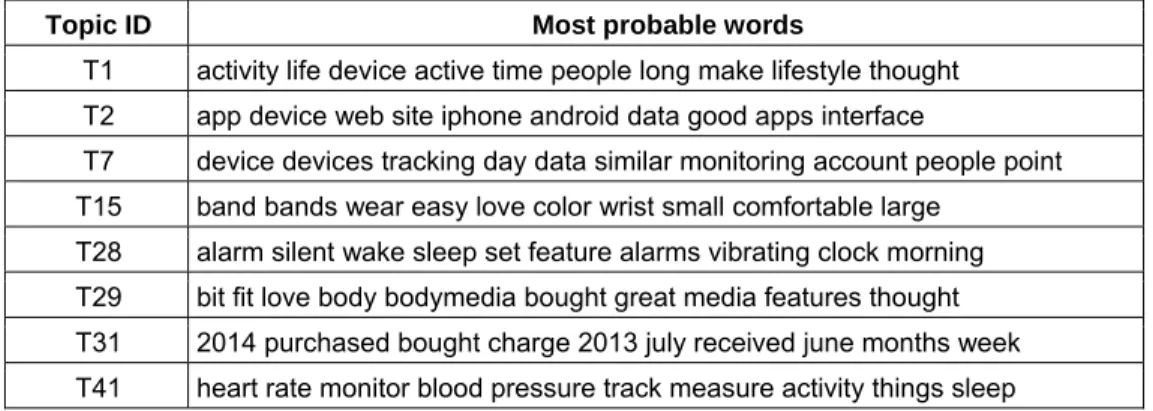
6. Removing HTML tags and other technical symbols, which may stem from Web scraping activity. Table 2 shows an excerpt of the results of the initial LDA analysis. It displays the most probable words for eight selected topics and reveals several data-quality issues that hindered us from properly interpreting the topics. For example:
1. The most probable terms in topic 7 were “device” and “devices” and in topic 15 “band” and “bands”. To harmonize these terms, we added a lemmatization step to our preprocessing pipeline. 2. Many topics contained the words “fitbit”, “flex”, “fit”, and “bit” among the top-10 most probable
words (see, e.g., topic 29). This result is not surprising because all reviews were about the Fitbit device. From a text-mining perspective, these words do not add new information to the reviews; on the contrary, they might even bias the statistical analysis or hinder the interpretation of results. Therefore, we eliminated those terms by adding them to the custom stop-word list.
3. Engaging with the vocabulary of the domain of interest (e.g., the features of a product under review) is crucial for interpreting and making sense of the results of any text mining study. For example, we spotted that topic 28 concerned the “silent alarm” function of the device. Unfortunately, the LDA algorithm treated the terms “alarm” and “silent” as independent terms. By modifying our model to include n-grams, we forced the algorithm to create a new composite term “silent_alarm”, which helped to better explain the topic. We observed the same problem for topic 41 (“heart”, “rate”, and “monitor” “heart_rate_monitor”; “blood” and “pressure”
“blood_pressure”).
4. Some customers provided lots of details in their reviews, such as the month and year of their purchase. Because the metadata already captured this information (date field), we removed number words.
Table 2. Exemplary Topics of Initial Topic Model (before data preparation)
Topic ID Most probable words
T1 activity life device active time people long make lifestyle thought T2 app device web site iphone android data good apps interface
T7 device devices tracking day data similar monitoring account people point T15 band bands wear easy love color wrist small comfortable large
T28 alarm silent wake sleep set feature alarms vibrating clock morning T29 bit fit love body bodymedia bought great media features thought T31 2014 purchased bought charge 2013 july received june months week T41 heart rate monitor blood pressure track measure activity things sleep
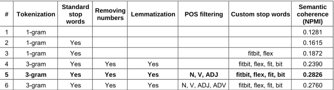
To fine-tune the topic model, we experimented with different data-preparation options, re-ran the LDA algorithm, and used an automated approach to evaluate the quality of the resulting descriptive topic model (see variations listed in Table 3). We applied Lau et al.’s (2014) approach to automatically evaluate the semantic coherence of a topic model by calculating how often pairs of terms from the top-n words of a topic co-occur within a narrow window (e.g., 10 words) sliding over a reference corpus (for detailed information about the technique, see Lau et al. (2014) and Newman et al. (2010)). In experiments the resulting normalized pointwise mutual information (NPMI) metric, which can range between -1 (worst) and +1 (best), was highly correlated with human judgments of semantic coherence (Pearson correlation between 0.84 and 0.98) (Lau et al., 2014). We calculated the NPMI score for different sets of preprocessing options using the original corpus of reviews as a reference corpus. The results indicate that configuration 5 in Table 3 (i.e., 3-gram tokenization, removal of standard stop words, removal of numbers, lemmatization, POS tagging (nouns, verbs, adjectives) and a small list of custom stop words (fitbit, flex, fit, bit)) produced the topic model with the best interpretability.
Volume 39 Paper 7 Table 3. Different Data Preparation Options and Their Effect on Semantic Coherence
# Tokenization
Standard stop words
Removing
numbers Lemmatization POS filtering Custom stop words
Semantic coherence
(NPMI)
1 1-gram 0.1281
2 1-gram Yes 0.1615
3 1-gram Yes fitbit, flex 0.1872
4 3-gram Yes Yes Yes fitbit, flex, fit, bit 0.2390
5 3-gram Yes Yes Yes N, V, ADJ fitbit, flex, fit, bit 0.2826
6 3-gram Yes Yes Yes N, V, ADJ, ADV fitbit, flex, fit, bit 0.2760
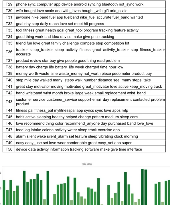
Table 4 summarizes the final topic model by showing the top-10 most probable words for each of the 50 topics, and Figure 9 visualizes the overall distribution of topics across the corpus (i.e., the higher the probability of a topic, the more reviews talked about the topic).
Table 4. Topics of Final Topic Model
Topic Most probable words
T1 day step week work walk time steps_day walking couple end
T2 wear shower water time band love charge comfortable wear_shower swimming T3 weight lost pound lose loss week lb lost_pounds month weight_loss
T4 minute active activity walking step mile running active_minutes run track T5 wrist wearing wear time zip pedometer put thing lost clip
T6 heart rate heart_rate monitor rate_monitor heart_rate_monitor blood pressure blood_pressure pedometer T7 sleep tracking time night step sleep_tracking day pattern feature hour
T8 instruction work set site website find web user time figure
T9 gift love christmas bought husband daughter received birthday gave present T10 motivated move love day walk make step moving motivate keeps_motivated
T11 product great recommend great_product love recommend_product good excellent not_recommend good_product T12 charge charger charging hold month unit battery issue hold_charge problem
T13 sleep mode sleep_mode put time tap tapping put_sleep forget turn
T14 track sleep step keep_track track_steps love activity track_sleep great keeps_track T15 stair ultra count track climbed step big flight deal floor
T16 make time made long thing life love make_sure aware change T17 band wrist difficult clasp put hard wristband snap time bracelet
T18 return amazon day product item week charge worked purchased happy T19 work great works_great not_work item advertised fine love idea not_great
T20 working stopped month stopped_working week worked charging bought quit stopped_charging T21 accurate step hand pedometer wear stride setting distance dominant wrist
T22 lost band clasp wrist fell time design wristband fall secure
T23 calorie burned calories_burned track burn step day many_calories eat weight T24 month year mine broke le bought strap issue lasted warranty
T25 app iphone sync ipad iphone_app work io apple android computer T26 light force display time band step progress watch dot show
T27 step count arm movement accurate hand counting walking count_steps moving T28 activity sleep monitor level daily activity_level activity_sleep day aware daily_activity
Volume 39 Paper 7 Table 4. Topics of Final Topic Model
T29 phone sync computer app device android syncing bluetooth not_sync work T30 wife bought love scale aria wife_loves bought_wife gift aria_scale
T31 jawbone nike band fuel app fuelband nike_fuel accurate fuel_band wanted T32 goal day step daily reach love set meet hit progress
T33 tool fitness great health goal great_tool program tracking feature activity T34 good thing work bad idea device make give price tracking
T35 friend fun love great family challenge compete step competition lot
T36 tracker sleep_tracker sleep activity fitness great activity_tracker step fitness_tracker accurate T37 product review star buy give people good thing read problem
T38 battery day charge life battery_life week charged time hour low
T39 money worth waste time waste_money not_worth piece pedometer product buy T40 step mile day walked many_steps walk number distance see_many steps_take T41 great stay motivator moving motivated great_motivator love active keep_moving track T42 band wristband wrist month broke large week small replacement wrist_band
T43 customer service customer_service support email day replacement contacted problem product T44 fitness pal fitness_pal myfitnesspal app syncs sync love apps mfp
T45 habit active sleeping healthy helped change pattern medium sleep care T46 love recommend thing color recommend_anyone day purchased band love_love T47 food log intake calorie activity water sleep track exercise app
T48 alarm silent wake silent_alarm set feature sleep vibrating clock morning T49 easy easy_use set love wear comfortable great easy_set app super T50 device data activity information tracking software make give time interface
Figure 9. Overall Topic Distribution
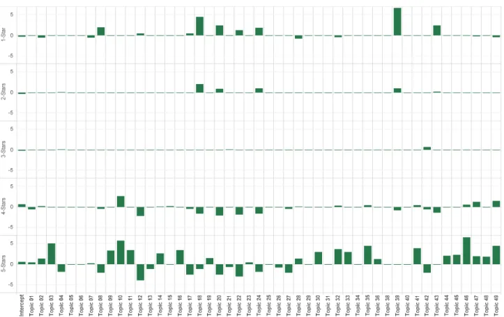
For the modeling phase’s final step, we quantified the influence of the identified topics (independent variables) on user satisfaction (dependent variable). To do so, one can apply different regression analysis techniques. The most common choice would be to use a linear ordinary least squares (OLS) regression; however, the star ratings used an ordinal and not continuous scale. Consequently, ordered logistic regression would be a better choice. Yet, testing the proportional odds assumption of ordered logistic regression against our dataset showed that the topics’ influence on star rating varied between levels of star rating—a consequence of the J-shaped distribution of user satisfaction. Hence, we decided to use multinomial logistic regression, which treats the different levels of our dependent variable (i.e., one, two,
Volume 39 Paper 7
three, four, five stars) as unordered categories. Consequently, it produces separate coefficients for each level of the dependent variable; in our example, five coefficients for each of the 50 topics (i.e., 250 coefficients). To manage the complexity of the resulting model and to increase its interpretability, we chose least absolute shrinkage and selection operator (LASSO) to fit the model to the data. LASSO is a linear regression method that performs variable selection by shrinking the coefficients of uninfluential independent variables to exactly zero, which produces a model that only includes the most important independent variables for explaining the dependent variable (Hastie, Tibshirani, & Friedman, 2013). Figure 10 visualizes the coefficients of the LASSO regression model3. For example, the analysis revealed
that the top-five topics associated with a five-star rating were: topic 46 (“recommend to others”), topic 10 (“motivation to move”), topic 3 (“losing weight”), topic 35 (“competing with friends”), and topic 49 (“easy to use”). In contrast, the top-five topics associated with a one-star rating were: topic 39 (“negative cost/benefit ratio”), topic 18 (“Amazon’s product return policy”), topic 20 (“malfunction”), topic 43 (“customer service”), and topic 8 (“operating instructions”). The goodness-of-fit of the estimated model, as measured by the fraction of deviance explained by the model, amounted to 0.26 and its classification accuracy to 0.57.
Figure 10. Coefficients of LASSO Multinomial Logistic Regression
4.4
Interpretation
The last step comprised understanding and making sense of the discovered topics and their influence on user satisfaction. One can uncover the meaning of a topic by analyzing its most probable terms in combination with the associated most probable documents. Figure 11 shows a bubble chart of the word distribution of topic 3. The size and color of the bubbles both represent the probability of a given term in a given topic. A first labeling of this topic may yield “losing weight”. However, to verify whether the initial interpretation based on word probabilities makes sense, one should thoroughly investigate the associated documents. Table 5 confirms that customers have happily reported their success stories about losing weight with the help of their Fitbit device. Overall, the first and second authors independently interpreted
3 To select the most appropriate lambda parameter for the lasso penalty, we performed a grid search using 10-fold cross validation,
Volume 39 Paper 7
and labeled all 50 topics and, apart from minor wording differences, reached an inter-coder agreement of 84 percent.
Figure 11. Most Probable Words of Topic 3 (“Losing Weight”)
Table 5. Reviews Most Strongly Associated with Topic 3 (“Losing Weight”)
Probability Text Star rating
0.81 Helped me reach my weight loss goals and maintain my weight for 6 weeks now. Has
become part of me 24/7. 5
0.78 The FitBit has helped my make a total lifestyle change. I've lost 27 pounds so far, and
counting. 5
0.78
I AM TRYING TO LOSE WEIGHT FOR 3 EVENTS THIS SUMMER. THE FITBIT HAS HELPED WITH MY MOTIVATION A LOT. I HAVE NOT LOST A LOT OF WEIGHT. BUT WHEN SOMEONE SEES ME AND THEY HAVE NOT SEEN ME FOR A WHILE THEY SAY "YOUR GETTING SKINNY". I WOULD RECOMEND THIS ITEM TO ANYONE WANTING TO GET MOTIVATION TO MOVE AND GET FIT.
5
0.76 I love mine. It helped me lose 20 lbs. 5
0.72
I bought this at the end of July 2014. I wanted to track what I was eating, loose about 15 pounds, and increase my general fitness. I will be 60 years old in May. I have changed my lifestyle, I eat less food and things that are more healthy. I have lost about 33 pounds as I just kept going. I feel better than I have in 20 years, my general fitness is outstanding now since I have paid attention. The Fitbit Flex has been an integral part of my program. It's an outstanding value to accomplish all of this for me. The only problem, I need a lot of new clothes, my waist size decreased 4 inches, in a little over 3 months. I walk very briskly twice a day for my exercise. If you will learn how to use the Fitbit, it is really quite simple and very worthwhile.
5
To make sense of the discovered topics against the background of existing theory, we tried to map the interpreted topics to theoretical constructs of theories from the field of technology acceptance; in particular, we focused on the technology acceptance model (TAM) (Venkatesh & Davis, 2000; Venkatesh, Morris, Davis, & Davis, 2003) and the IS success model (e.g., DeLone & McLean, 2003). Similar to interpreting topics through labeling, the first and second authors mapped topics with constructs independently based on a list of theoretical definitions (Table 7). The coders reached an inter-coder agreement of 86 percent.
Table 6 shows a sample result of the mapping process. The coders unambiguously mapped most of the topics with extant constructs. For example, they mapped “losing weight” (topic 3) with the construct of net
Volume 39 Paper 7
benefits because losing weight seems to be an indirect consequence—through increased physical activity—of using the Fitbit Flex device. And they mapped customer comments about the “accuracy of activity tracking” (Topic 4) with the construct of accuracy, a subconstruct of information quality construct in the IS success model, and “Amazon’s product return policy” (Topic 18) with service quality. With regards to TAM, they mapped topic 49 “easy to use” with the ease of use construct, and the Topic 1 “step tracking” with usefulness because it represents one of the device’s core features.
Table 6. Definitions of Constructs Related to User Satisfaction
Construct Subconstruct Definition Source
System
quality Desirable characteristics of an information system.
Petter, DeLone, & McLean (2013) Reliability Dependability of the system’s operation. Wixom & Todd (2005)
Flexibility The way the system adapts to users’ changing demands. Wixom & Todd (2005) Integration The way the system allows one to integrate data from various sources. Wixom & Todd (2005) Accessibility The ease with which one can access or extract information from the system. Wixom & Todd (2005) Timeliness Degree to which the system offers timely responses to requests for information or action. Wixom & Todd (2005) Information
quality
Desirable characteristics of the systems’ outputs (content, reports, dashboards).
Nelson, Todd, & Wixom (2005) Completeness Degree to which the stored information represents all possible states relevant to the user population. Nelson, Todd, & Wixom (2005) Accuracy Degree to which information is correct, unambiguous, meaningful, believable, and consistent. Nelson, Todd, & Wixom (2005) Format Degree to which information is presented in a manner that is understandable and interpretable to the user and, thus, aids
users in completing tasks.
Nelson, Todd, & Wixom (2005) Currency Degree to which information is up-to-date or the degree to which the information precisely reflects the current state of the
world that it represents.
Nelson, Todd, & Wixom (2005) Service
quality
The quality of support that system users receive from the IS department and IT support.
Nelson, Todd, & Wixom (2005) Net benefits
Extent to which an information system contributes to the success of individuals, groups, organizations, industries, and nations.
Nelson, Todd, & Wixom (2005) Usefulness Degree to which individuals think that using a particular system will enhance their job performance. Davis, Bagozzi, & Warshaw (1989) Ease of Use Degree to which individuals think that using a particular system will be free of effort. Davis, Bagozzi, & Warshaw (1989)
User
satisfaction Users’ level of satisfaction with the information system.
Petter, DeLone, & McLean (2013)
Overall, of the 50 topics identified, we mapped 14 with system quality, 12 with usefulness, six with net benefits, three with information quality, two with service quality, and two with ease of use—all antecedents of user satisfaction. We classified some of the remaining topics as indictors rather than antecedents of user satisfaction (topics 11, 33, and 46)4.In addition, we discovered eight topics that neither corresponded
to constructs of the IS success model or TAM. For instance, topic 39 “negative cost/benefit” or topic 31 “comparison with competitor products” do not have a theoretical equivalent in either of the two models. This finding may give rise to extend the existing theories or to develop entirely new theories—two goals beyond our purpose here.
4 Removing these three topics from the explanatory regression model only slightly reduced its goodness-of-fit and predictive
Volume 39 Paper 7 Table 7. Definitions of Constructs Related to User Satisfaction
Topic Most probable
terms Exemplary highly associated review sentences Label
Mapping to existing constructs
T1
day step week work walk time steps_day walking couple end
I'm averaging about 12,350 steps a day. I look forward to the day when I can use it on my early and late night runs. When I first got it I was lucky to get 4000 steps a day because most of my job is at a desk. I had to really work to get to the 10k target. I've had it now for a couple of months and have increased my target to 12k daily.
Step tracking Usefulness (Venkatesh & Davis, 2000) T3
weight lost pound lose loss week lb lost_pounds month
weight_loss lose_weight helped love eat losing year day goal lost_lbs
Helped me reach my weight loss goals and maintain my weight for 6 weeks now. Has become part of me 24/7. The FitBit has helped my make a total lifestyle change. I've lost 27 pounds so far, and counting.
Losing weight Net benefits (DeLone & McLean, 2003) T4
minute active activity walking step mile
running active_minutes run
track exercise accurate record bike
register weight measure treadmill
hour
I like the fitbit and enjoy seeing my steps on the rise. However, I often use the elliptical or the bicycle and it does not record that activity. Only works with walking. That's disappointing to me.
Just today walked with fit bit on a GPS measured 3 mile trail. Took me 48 minutes. Fit bit registered 2.5 miles and 23 minutes of activity. So it's ok if 50% accuracy is acceptable to you. Accuracy of activity tracking Information quality -> accuracy (DeLone & McLean, 2003) T9
gift love christmas bought husband daughter received birthday gave present
son day christmas_gift purchased year bought_husband sister mother loved
I bought it as a Christmas present for my brother in law and he loves it.
I gave the item as a gift. I think she likes it as much as I do mine, that I received as a gift.
Fitbit as a gift No corresponding IS construct identified T10
motivated move love day walk make step moving motivate keeps_motivated
It has made me much more aware that I need to move more during the day. It has helped me get more fit. Love it! Really motivates you to get up and get moving! Looking forward to getting a lot of use out of it!
Motivation to move Net benefits (DeLone & McLean, 2003) T12 charge charger charging hold month
unit battery issue hold_charge problem
not_charge not_hold time charged usb
work
not_hold_charge light contact
Worked for about six months before battery refused to take a charge. After many emails, the mfr did send a new one. Now, six months later, the same thing - battery will not charge.
Love my Fitbit. However, 2.5 month in and I'm having major battery charging issues. Hoping to get resolved ASAP. Battery charging issues System quality -> reliability (DeLone & McLean, 2003) T18
return amazon day product item week charge worked purchased happy refund returned disappointed policy replacement bought purchase buy warranty
The fitbit won't charge and amazon won't accept returns after 30 days. This is the second fitbit received after the first one also didn't charge.
This item only worked for less than 90 days, want to return to amazon for replacement, not allowing a return.
Amazon’s product return policy Service quality (DeLone & McLean, 2003)
Volume 39 Paper 7 Table 7. Definitions of Constructs Related to User Satisfaction
T31
jawbone nike band fuel app fuelband nike_fuel accurate
fuel_band wanted
Bought this and Jawbone simultaneously. This is much better on performance than Jawbone. Its app is better and the blue tooth connectivity helps.
I've owned a Nike+ band and wore it for almost a year. The flex is smaller, has interchangeable bands (if you can find them) and has a ton of more features over Nike's band. Compariso n to competitor products No corresponding IS construct identified T39
money worth waste time waste_money not_worth piece pedometer product
buy worth_money thing save work
expensive junk not_waste spent
disappointed
I repeat do not waste your money :(Do not waste your money. Unless you have money to throw away. way too expensive for what it can do and for how inaccurate it is. I can get the same thing for free or real cheap Negative cost/benefi t ratio No corresponding IS construct identified T43 customer service customer_service support email day
replacement contacted problem
product
Customer service is awful. Defective product, and the Fit Bit company makes you jump through so many hoops to repair or replace a $100 product, that it hopes you just give up. I