An efficient multilocus mixed model
framework for the detection of small and
linked QTLs in F2
Article
Published Version
Creative Commons: Attribution 4.0 (CCBY)
Open Access
Wen, Y.J., Zhang, Y.W., Zhang, J., Feng, J.Y., Dunwell, J.
M. and Zhang, Y.M. (2018) An efficient multilocus mixed
model framework for the detection of small and linked QTLs in
F2. Briefings in Bioinformatics. ISSN 14675463 doi:
https://doi.org/10.1093/bib/bby058 Available at
http://centaur.reading.ac.uk/78290/
It is advisable to refer to the publisher’s version if you intend to cite from the
work. See Guidance on citing
.
To link to this article DOI: http://dx.doi.org/10.1093/bib/bby058
Publisher: Oxford University Press
All outputs in CentAUR are protected by Intellectual Property Rights law,
including copyright law. Copyright and IPR is retained by the creators or other
copyright holders. Terms and conditions for use of this material are defined in
the End User Agreement
.
www.reading.ac.uk/centaur
Central Archive at the University of Reading
Reading’s research outputs online
An efficient multi-locus mixed model framework for
the detection of small and linked QTLs in F
2
Yang-Jun Wen, Ya-Wen Zhang, Jin Zhang, Jian-Ying Feng,
Jim M. Dunwell and Yuan-Ming Zhang
Corresponding author: Yuan-Ming Zhang, Crop Information Center, College of Plant Science and Technology, Huazhong Agricultural University, Wuhan 430070, China. Tel.:þ086 13505161564; E-mail: [email protected]; College of Agriculture, Nanjing Agricultural University, Nanjing 210095, China. Tel.:þ086 13505161564; Fax:þ086 25 84399091; E-mail: [email protected]
Abstract
In the genetic system that regulates complex traits, metabolites, gene expression levels, RNA editing levels and DNA methy-lation, a series of small and linked genes exist. To date, however, little is known about how to design an efficient framework for the detection of these kinds of genes. In this article, we propose a genome-wide composite interval mapping (GCIM) in F2. First, controlling polygenic background via selecting markers in the genome scanning of linkage analysis was replaced by estimating polygenic variance in a genome-wide association study. This can control large, middle and minor polygenic backgrounds in genome scanning. Then, additive and dominant effects for each putative quantitative trait locus (QTL) were separately scanned so that a negative logarithmP-value curve against genome position could be separately obtained for each kind of effect. In each curve, all the peaks were identified as potential QTLs. Thus, almost all the small-effect and linked QTLs are included in a multi-locus model. Finally, adaptive least absolute shrinkage and selection operator (adaptive lasso) was used to estimate all the effects in the multi-locus model, and all the nonzero effects were further identified by likelihood ratio test for true QTL identification. This method was used to reanalyze four rice traits. Among 25 known genes detected in this study, 16 small-effect genes were identified only by GCIM. To further demonstrate GCIM, a series of Monte Carlo simulation experiments was performed. As a result, GCIM is demonstrated to be more powerful than the widely used methods for the detection of closely linked and small-effect QTLs.
Key words:genome-wide composite interval mapping; small-effect QTL; linked QTLs; mixed linear model; multi-locus model; adaptive lasso
Yang-Jun Wenis a PhD Candidate in State Key Laboratory of Crop Genetics and Germplasm Enhancement at Nanjing Agricultural University, Nanjing,
China.
Ya-Wen Zhangis a PhD Candidate in the College of Plant Science and Technology at Huazhong Agricultural University, Wuhan, China.
Jin Zhangis an Associate Professor in State Key Laboratory of Crop Genetics and Germplasm Enhancement at Nanjing Agricultural University, Nanjing,
China.
Jian-Ying Fengis an Associate Professor in State Key Laboratory of Crop Genetics and Germplasm Enhancement at Nanjing Agricultural University,
Nanjing, China.
Jim M. Dunwellis a Full Professor in the School of Agriculture, Policy and Development at the University of Reading, United Kingdom.
Yuan-Ming Zhangis director of Crop Information Center and a Chutian Scholar Professor of Statistical Genomics in the College of Plant Science and
Technology at Huazhong Agricultural University, Wuhan, China.
Submitted:5 April 2018;Received (in revised form):5 June 2018
VCThe Author(s) 2018. Published by Oxford University Press.
This is an Open Access article distributed under the terms of the Creative Commons Attribution Non-Commercial License (http://creativecommons.org/ licenses/by-nc/4.0/), which permits non-commercial re-use, distribution, and reproduction in any medium, provided the original work is properly cited. For commercial re-use, please contact [email protected]
Briefings in Bioinformatics, 2018, 1–12
doi: 10.1093/bib/bby058
Introduction
Most complex traits are controlled by a few major genes with large effects plus a series of undetectable genes with small effects. When markers are introduced, some genes will be cap-tured by the markers in recombinant or linkage disequilibrium with quantitative trait loci (QTLs). Among these reported QTLs, most have small effects on complex traits and some are closely linked QTLs [1,2], for example, flowering time in maize [3] and growth rate in Arabidopsis [4]. Although QTL mapping has pro-ven to be useful for detecting major QTLs with relatively large effects, it may lack power in accurately modeling small-effect QTLs [5]. Additionally, closely linked QTLs might be mistakenly estimated as a single QTL with a larger effect at the wrong pos-ition if they have the same direction in effects, or they might be missed if their effects are in opposite directions [6]. We are now in the era of omics, which enables us to incorporate genetic variation in omics phenotypes into a QTL mapping framework. In expressional QTL (eQTL) mapping, most aretrans-eQTLs with small effects [7,8]. Similar results have been observed in the mapping of metabolites [9], RNA editing levels [10] and DNA methylation [11]. Because of the difficulty in detecting small-effect and closely linked QTLs, the genetic foundations of most complex and omics-related traits are not well understood.
To overcome the above issue, many attempts have been made during the past several decades. In biology, accurate phe-notypes and high-density molecular gephe-notypes are needed for many thousands of individuals to map small-effect and closely linked QTLs [2]. In statistics, many approaches have been pro-posed. In early studies, some markers associated with complex traits of interest were selected to control polygenic background in composite interval mapping (CIM) and its derivatives [12–16]. Subsequently, controlling polygenic background via the selec-tion of markers in the CIM was replaced by estimating all the marker variances or effects in one model [17–21]. To estimate these effects in one model, many penalization methods have been developed, for example, least absolute shrinkage and se-lection operator (lasso) [22], smoothly clipped absolute devi-ation [23] and empirical Bayes [24]. Although these penalizdevi-ation methods can handle a number of markers several times larger than the sample size, they will fail when the number of markers is significantly larger than the sample size, especially for ex-tremely high marker density. Recently, controlling polygenic background in linkage analysis has been replaced by estimating polygenic variance in genome-wide association studies [25–27]. However, this method cannot be directly applied in F2.
Goddardet al.[28] have proposed a method to treat marker effects as random and described several advantages of the ran-dom model approach over the fixed model treatment. This view-point has been further confirmed by Wanget al.[27,29]. If marker effects in F2are treated as random, five variance components must be estimated in genome scanning. Although Wanget al.[27] have proposed a new method for the detection of small and close-ly linked QTLs in the backcross generation, this method does not work in F2. This is because there are five variance components to be estimated. Clearly, this increases the difficulty of parameter es-timation and the calculation burden in genome scanning.
In this study, we propose a rapid and efficient multi-locus mixed linear model to detect small and linked QTLs in F2. To de-crease the number of variance components estimated in gen-ome scanning, three measures were used. The first is to separately scan additive and dominant effects. The second is to fix the polygenic-to-residual variance ratio [30], and the last is to use the algorithm of Wenet al.[31]. To increase the power in
the detection of small and linked QTLs, all the peaks in the negative logarithmP-value curve against genome position for additive or dominant effects were viewed as potential QTLs, and these potential QTLs were placed into one model for true gene identification. To confirm the benefit of the new method proposed in this study, yield and yield component traits in an ‘immortalized F2’ (IMF2) population derived from an elite rice hybrid [32] were reanalyzed by the new method, while a series of simulation studies were conducted to show the advantage of the new method over those currently used.
Results
Mapping QTLs for yield and yield component traits in an IMF2
In this study, we reanalyzed four rice traits described in Zhou et al.[32] using four methods. The four traits are yield per plant (YIELD), tillers per plant (TILLER), grains per panicle (GRAIN) and thousand grain weight (KGW). The four methods were genome-wide composite interval mapping (GCIM)-random, GCIM-fixed, CIM and inclusive CIM (ICIM). GCIM-random and GCIM-fixed are the GCIM under the situations of random and fixed QTL effects, respectively. All the results are listed inTable 1,Supplementary
Tables S1–S2andFigure 1,Supplementary Figures S1–S3.
A total of 104, 56, 20 and 46 QTLs for the aforementioned four traits were detected by GCIM-random, GCIM-fixed, ICIM and CIM, re-spectively (Supplementary Table S1). Clearly, the number of QTLs identified by the new methods (GCIM-random and GCIM-fixed) was much higher than that identified by the current ICIM and CIM meth-ods. For example, 24 and 21 QTLs for GRAIN were detected, respect-ively, by GCIM-random and GCIM-fixed while only 4 and 10 QTLs were identified, respectively, by ICIM and CIM. The same trend was also observed for the other traits. Among all the 226 QTLs, 176 (78%) had<5% proportions of phenotypic variance explained by each QTL. Among the 50 large QTLs, 11 were detected simultaneously by sev-eral methods. The QTL genotypic information for each trait was used to conduct a multiple linear regression analysis, and the corre-sponding Akaike’s information criteria (AIC) values were calculated. A smaller AIC value indicates a better model fit. As a result, the min-imum AIC value for each trait was from GCIM, and the current methods had the maximum AIC values (Supplementary Table S2). For example, the AIC value for TILLER was 838.44 for GCIM-random, 850.17 for GCIM-fixed, 853.41 for CIM and 913.91 for ICIM.
In the proximity of the QTLs detected by GCIM-random, GCIM-fixed, ICIM and CIM methods, a total of 24, 9, 7 and 7 pre-viously reported genes were found to be associated with the aforementioned four traits, respectively (Table 1,Figure 1, and Supplementary Figures S1–S3). Clearly, GCIM detected more pre-viously reported genes when compared with all the other meth-ods. Among the aforementioned genes, five genes were simultaneously detected by all the four methods, i.e.GS3[33] andGW5[34] for KGW,Ghd7[35] andGUDK[36] for YIELD,Gn1a [37] for GRAIN andGhd7[35] for GRAIN were identified by GCIM-random, GCIM-fixed and CIM. Note that all the five genes have almost large effects (r2>5%), and the other genes have small effects (r2<2.5%) with an exception of geneTAC1(r2¼5.81). More importantly, all the small-effect known genes were detected by GCIM-random rather than by the current methods (CIM or ICIM). For example,Gn1a[37],OsLSK1[38],NOG1[39], GW2 [40], AFD1 [41], GS3 [33], GIF1 [42], GW5 [34], d3 [43], OsglHAT1[44], OsAPO1[45],PROG1[46] andPAY1[47] for YIELD; d3[43],OsLIC[48] andATC1[49] for TILLER;NOG1[39] for GRAIN
Table 1. Previously reported genes for yield/plant (YIELD), tillers/plant (TILLER), grains/panicle (GRAIN) and thousand grain weight (KGW) in rice using G CIM-random, GCIM-fixed, ICIM and CIM methods Trait Gene MSU_locus Chr Pos (Mb) M arker associa ted GCIM-random (A) GCIM-fixed (B) ICIM (C) CIM (D) Reference LOD Add Dom r 2(%) LOD Add Dom r 2(%) LOD Add Dom r 2(%) LOD Add Dom r 2(%) YIELD Gn1a LOC_Os01g10110 1 5.667 Bin40 10.52 1.29 0.00 1.13 Ashika ri et al. [ 37 ] 1OsLSK1, LSK1 1LOC_Os01g47900 1 28.397 Bin135 12.79 1.47 0.00 1.71 1Zou et al. [ 38 ] 2NOG1 2LOC_Os01g54860 2Huo et al. [ 39 ] GW 2 LOC_Os02g14720 2 8.810 Bin268 3.00 0.00 0.58 0.13 Son g et al. [ 40 ] AFD1, OsG1L6, TH1 LOC_Os02g56610 2 34.340 Bin339 12.82 0.00 1.40 0.77 Li et al. [ 41 ] 34.738 Bin344 10.68 0.00 1.28 0.64 GUD K, OsRLCK10 3 LOC_Os03g08170 3 4.894 A, B Bin378 A, B, D 5.41 0.00 0.84 0.28 5.91 0.00 1.86 2.20 4.72 0.18 3.06 7.23 4.33 0.78 3.17 6.44 Rame gowda et al. [ 36 ] 4.9 D,5 C Bin378 Bin379 C GS3 LOC_Os03g29380 3 15.597 Bin433 6.21 0.86 0.00 0.58 Fa n et al. [ 33 ] GIF1 LOC_Os04g33740 4 19.644 Bin617 13.39 0.00 1.51 0.90 Wa ng E et al. [ 42 ] GW 5/qsw5 LOC_Os05g09520 5 3.438 Bin722 5.38 0.87 0.00 0.60 Liu et al. [ 34 ] d3 LOC_Os06g06050 6 3.291 Bin855 6.23 0.93 0.00 0.68 Ishika wa et al. [ 43 ] 1OsglHAT1, GW 6a 1LOC_Os06g44100 6 24.309 Bin936 12.39 0.00 1.37 0.74 1Song et al. [ 44 ] 2Kyok o et al. [ 45 ] 2OsAPO1, SCM2 2LOC_Os06g45460 PROG1 LOC_Os07g05900 7 2.817 Bin989 10.58 1.31 0.00 1.36 Tan et al. [ 46 ] Ghd7 LOC_Os07g15770 7 8 A, C Bin1003 Bin1004 A, C 44.84 2.79 3.41 10.75 7.38 2.05 2.21 8.44 3.29 0.22 2.52 5.10 6.91 2.32 2.63 17.17 Xue et al. [ 35 ] 12 B Bin1007 Bin1008 B 12.4 D Bin1007 D PAY1 LOC_Os08g31470 8 20.696 Bin1143 8.85 1.10 0.95 1.31 Zhao et al. [ 47 ] TILLER d3 LOC_Os06g06050 6 4 A Bin859 Bin860 A 8.18 0.00 0.56 2.44 8.28 0.00 0.63 3.64 6.51 0.26 0.84 0.47 Ishika wa et al. [ 43 ] 5.164 B, 5.2 D Bin867 B, D OsLIC , OsC3H46, 66LIC LOC_Os06g49080 6 24.666 Bin938 2.86 0.25 0.00 0.93 Wa ng L et al. [ 48 ] TAC1, OsTAC1, Spk LOC_Os09g35980 9 19.55 A, B Bin1262 A, B 4.34 0.24 0.80 5.81 3.39 0.00 0.35 1.15 Yu et al. [ 49 ] 5.761 B Bin42 B GRAIN Gn1a LOC_Os01g10110 1 6 C Bin43 Bin44 C 5.45 4.06 2.88 3.31 5.44 4.66 1.18 3.04 6.11 6.00 2.69 6.00 5.58 6.01 3.08 3.11 Ashika ri et al. [ 37 ] 6.04 A, 6.2 D Bin44 A, D NOG1 LOC_Os01g54860 1 28.442 Bin136 4.76 3.23 0.00 1.68 Huo et al. [ 39 ] PROG1 LOC_Os07g05900 7 7 Bin998 Bin999 10.65 8.53 2.46 10.89 Tan et al. [ 46 ] Ghd7 LOC_Os07g15770 7 8.4 D, 8.407 A Bin1003 D, Bin1004 A 15.22 3.40 5.13 3.96 14.48 6.79 5.72 8.45 10.81 8.20 5.37 18.14 Xue et al. [ 35 ] 8.756 B Bin1005 B KGW GS3 LOC_Os03g29380 3 16.224 A, 16.7 D Bin437 A, Bin438 D 15.02 0.54 0.00 4.30 6.39 0.33 0.38 2.63 28.06 0.98 0.15 16.00 21.06 1.19 0.30 16.83 Fa n et al. [ 33 ] 17 B, C Bin440 Bin441 B, C GW 5/qsw5 LOC_Os05g09520 5 5 A, B, C, 5.3 D Bin728 Bin729 A, B, C, Bin729 D 33.11 1.00 0.00 14.76 33.56 0.97 0.01 13.84 25.01 0.96 0.16 13.78 13.65 0.96 0.23 15.94 Liu et al. [ 34 ] IPA1 LOC_Os08g39890 8 2 5 C1 Bin1151 Bin1152 C 15.75 0.40 0.15 2.87 Jiao et al. [ 50 ] 28 C2 Bin1175 Bin1176 C 5.08 0.25 0.00 0.96 8.25 0.38 0.00 2.13 210.11 0.15 0.17 4.80 28.118 A, B Bin1176 A, B The individuals with missing phenotypes were excluded. The critical value for significance was LOD 2 : 5 for all the methods. The data set was derived from Zhou et al. (2012). chr: chromosome; LOD: logarithm of odds.
andIPA1[50] for KGW. This means that GCIM-random has high power for the detection of small-effect QTLs or genes.
Monte Carlo simulation studies
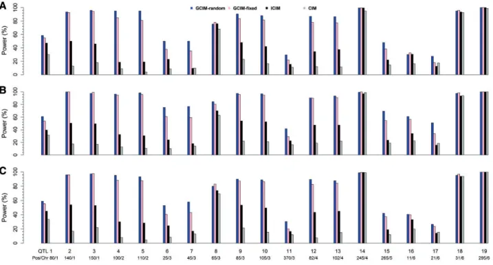
To validate the new method, a series of Monte Carlo simulation experiments was carried out. In the first experiment, 19 QTLs were simulated in an F2population of 400 individuals, each with 481 markers. All the interval lengths between adjacent markers were 5 cM and the number of replicates was 200. Each sample was analyzed by GCIM-random, GCIM-fixed, ICIM and CIM. As a result, the average power for the four methods was 73.42%, 67.71%, 43.39% and 29.97%, respectively (Figure 2 and Supplementary Table S3). When additive polygenic background (r2¼0.05) was added to the first simulation experiment, the average power for the four methods in the second simulation experiment was 83.63%, 78.42%, 47.47% and 33.16%, respectively (Figure 2andSupplementary Table S3). When normal distribu-tion for residual error in the first experiment was replaced by log-normal distribution in the third simulation experiment, average power for the four methods was 74.89%, 71.11%, 47.03% and 30.95%, respectively (Figure 2andSupplementary Table S3). Clearly, GCIM-random has the highest average power in all three simulation experiments. If a pairedt-test was used to test the significance of statistical power between new (GCIM-ran-dom and GCIM-fixed) and current (CIM and ICIM) methods, the new methods were significantly better than the current meth-ods; GCIM-random was significantly better than GCIM-fixed, indicating the highest power from GCIM-random (Table 2).
The accuracy of QTL effect estimation was measured by mean absolute deviation (MAD). Smaller MAD means higher
accuracy of parameter estimation. As a result, the average MADs for the four methods were 0.42760.351 (additive) and 0.26660.304 (dominant), 0.42960.361 and 0.23160.314, 0.42160.225 and 0.40560.105 and 0.63960.376 and 0.59260.288, respectively, in the first simulation experiment; 0.54860.401 and 0.31660.336, 0.50960.410 and 0.25460.331, 0.53860.208 and 0.43760.150 and 0.78960.389 and 0.66160.343, respectively, in the second simulation experi-ment; and 0.40360.330 and 0.24560.291, 0.40460.348 and 0.22360.308, 0.52960.255 and 0.45260.152 and 0.61160.372 and 0.58560.287, respectively, in the third simulation experi-ment (Suppleexperi-mentary Table S4). Clearly, GCIM-random and GCIM-fixed have relatively small average MADs in all three simulation experiments. If a pairedt-test was used to test the significance of the aforementioned accuracies between new (GCIM-random and GCIM-fixed) and current (CIM and ICIM) methods, the new methods had significantly lower MADs than the current methods, especially for dominant effects; GCIM-fixed had significantly lower MADs than GCIM-random (Table 2). This indicates that GCIM has higher accuracy in the estimation of QTL effects than the current methods.
The false positive rate (FPR) can be used to assess the per-formance of a method. The FPR results in the first simulation experiment are shown inFigure 3. The significance level (a) was set from 1e-8 to 1e-2.5, and the FPR slightly increased with the increase in theavalue (Figure 3). Whenawas set at 0.0032 (1e-2.5), the FPR values for GCIM-random, GCIM-fixed, ICIM and CIM were 0.4404%, 0.1722%, 0.1000% and 0.0211%, respectively.
In the three simulation experiments and real data analysis, the running times for the four methods were recorded and are
listed inSupplementary Table S5. The results show that ICIM has the minimum running time followed by GCIM-fixed and GCIM-random, and CIM has the maximum running time in real data analysis, indicating the moderate running time of the GCIM. Note that GCIM-fixed is faster than GCIM-random. This is reasonable, because four variance components in GCIM-random need to be estimated while only three variance compo-nents in the GCIM-fixed need to be estimated.
We used the IMF2population of an elite rice hybrid as a real ex-ample to demonstrate the several methods, while we conducted Monte Carlo simulation studies on the F2population to compare their differences. In reality, the genome structures of both IMF2and F2are not exactly the same in all respects. If IMF2is derived from doubled haploid lines, named IMF2-DH, there are no differences be-tween them, because the recombinant rate (r) between two adjacent markers in F2is the same as that in IMF2-DH. If IMF2is derived from recombinant inbred lines, named IMF2-RIL, however, the differences exist, because the recombinant rate between two adjacent markers is 2r/(1þ2r) in IMF2-RIL rather thanrin F2. More recombinant in IMF2-RIL will increase the power and accuracy of QTL detection. To validate the aforementioned deduction, we performed an additional simulation experiment to compare the results of QTL mapping in F2 and IMF2. All the results are listed inSupplementary Tables S6–S9. We found almost no significant differences between F2and IMF2-DH (Supplementary Table S6). However, the powers for linked QTLs in IMF2-RIL were significantly higher than those in both F2and IMF2-DH (Supplementary Table S6), and the FPR in IMF2-RIL was slightly less than those in both F2and IMF2-DH (Supplementary Table S9).
Discussion
Genetic reasons why GCIM-random has high power in the detection of QTLs
The 19 simulated QTLs mentioned above can be divided into three types: small (QTL1, QTL11and QTL15), large (QTL14and QTL19) and
linked (QTL2 QTL10, QTL12 QTL13 and QTL16 QTL18). As described above, GCIM-random has 5.71%, 30.03% and 43.45% higher power than GCIM-fixed, ICIM and CIM, respectively, in the first simulation experiment (Figure 2,Table 2, and Supplementary Table S3). To make clear the reasons that result in significant dif-ference in statistical power across various methods, we summar-ized the results from small, large and linked QTLs. We found that, for large-effect QTLs, GCIM-random has 0.0%, 0.0% and 2.75% higher power than GCIM-fixed, ICIM and CIM, respectively; for small-effect QTLs, GCIM-random has 6.83%, 17.17% and 26.83% higher power than GCIM-fixed, ICIM and CIM, respectively; for linked QTLs, GCIM-random has 6.29%, 37.07% and 52.82% higher power than GCIM-fixed, ICIM and CIM, respectively. This indicates the similar power of the four methods for large-effect QTLs, signifi-cantly different values between the current methods and GCIM-random for small-effect QTLs, and very significantly different val-ues between the current methods and GCIM-random for linked QTLs. The same trends are also found in the other two simulation experiments. These results are further confirmed by real data ana-lysis in this study. For example, five large-effect QTLs are detected simultaneously by the four methods (Table 1); among all the QTLs identified from GCIM-random and GCIM-fixed, 147 (91.88%) are small-effect (<5%) (Supplementary Table S1). In conclusion, the high power for the GCIM-random is derived from its high power in the detection of small and linked QTLs.
The advantages of GCIM-random are favorable in the map-ping of gene expression levels, metabolites and epigenetic in-heritance indicators. As we know, one of the most remarkable findings in eQTL mapping is that the most strong eQTLs are found to be near the target gene [8], and the proportion of these cis-acting eQTLs is approximately one third [7]. This means that mosttrans-eQTLs have small effects. Similar conclusions can be found in the mapping of metabolites [9] and epigenetic inherit-ance indicators [10,11]. Thus, GCIM-random can improve the power in the detection of expressional, metabolic and epigenet-ic QTLs.
Figure 2.Comparison of statistical powers of QTL detection in the first (A), second (B) and third (C) simulation experiments using CIM, ICIM, GCIM-random and
GCIM-fixed methods.
The advantages of GCIM-random over the current methods
As described in Kroymann and Mitchell-Olds [4] and Mackay et al.[2], it is difficult for the widely used QTL mapping methods to detect small and linked QTLs. However, this situation has been significantly changed in this study; for example, a large number of small-effect QTLs have been identified in rice real data analysis by GCIM-random. The reasons are as follows. First, all the peaks in the negative logarithm P-value curve against genome position for additive or dominant effects are viewed as potential QTLs and placed into a multi-locus genetic model for true QTL identification. In the widely used QTL map-ping methods, the peaks of small or linked QTLs in the LOD curve exist. Although their LOD scores may be less than the crit-ical value of significant QTL, putting all the potential QTLs in one genetic model can increase the possibility of detecting small and linked QTLs. The results are consistent with those in Kaoet al.[14], Xu [18], Wanget al.[51] and Wanget al.[27]. Then, controlling polygenic background via selecting markers in QTL mapping is replaced by estimating polygenic variance in a genome-wide association study (GWAS). Although CIM and ICIM can control the background of polygenes with large and in-dividual moderate effects, GCIM-random may control the back-ground of polygenes with large, moderate and small effects. Note that polygenic background control has been adopted in Bernardo [25], Xu [26] and Wang et al. [27]. However, GCIM-random is based on the new algorithm of Wenet al.[31], multi-locus genetic model and adaptive lasso.
In the ICIM and CIM, additive and dominant effects for each putative QTL in the genome are simultaneously estimated. However, the two effects are separately detected in this study. In doing so, the number of variance components to be esti-mated in GCIM-random will decrease from five to three so that the algorithm of Wenet al.[31] can be directly adopted. This sol-ves the difficulty of parameter estimation in F2. This is reason-able because the two effects in F2are orthogonal. In addition, real data analysis and simulation studies provide the evidence for this treatment. In addition, we find one unexpected phe-nomenon in real data analysis. That is, two falsely linked QTLs (Bin1004 and Bin1006Bin1007 on chr 7) are found by GCIM-random in one neighborhood to be associated with YIELD. This is because only one QTL is detected by CIM and ICIM. To make clear the position and effects of the true QTL, we scanned this neighborhood by CIM [52] (http://cran.r-project.org/web/pack ages/qtl/). As a result, this QTL is located between Bin1003 and Bin1004. This kind of treatment has been incorporated into our GCIM software.
In the CIM, we frequently find several peaks around one true QTL. In this situation, we cannot distinguish one QTL from mul-tiple linked QTLs. In the GCIM-random, this situation can be avoided. This is because all the potential QTLs are placed into one genetic model, and their effects are estimated by shrinkage estimation (adaptive lasso). If there is only one true QTL in one neighborhood, only one nonzero effect estimate is obtained.
As compared with GCIM-random, GCIM-fixed has slightly higher accuracy in the estimation of QTL effects and takes less running time. However, GCIM-random has higher power in the detection of small and linked QTLs. The Monte Carlo simulation studies and real data analysis in this study provide the evidence for the detection of more small and linked QTLs (Supplementary Tables S1, S3 and S4). Thus, we recommend GCIM-random. Note that maximum likelihood (ML) and restricted maximum likelihood (REML) can be used to estimate
Table 2. The P -values in paired t-tests of differences for power and mean absolute deviation (MAD) between the new (GCIM-random and GCIM-fixed) and current (ICIM and CIM) methods QTL GCIM-random (A) and GCIM-fixed (B) GCIM-random (A) and ICIM (B) GCIM-random (A) and CIM (B) GCIM-fixed (A) and ICIM (B) GCIM-fixed (A) and CIM (B) Power MAD (Add) MAD (Dom) Power MAD (Add) MAD (Dom) Power MAD (Add) MAD (Dom) Power MAD (Add) MAD (Dom) Power MAD (Add) MAD (Dom) The first simulation experiment (phenotype ¼ mean þ 19 main-effect QTLs þ residual error w ith normal distribution) All 3e-04*** (5.711) 0.9645 ( 0.001) 0.0000*** (0.033) 1e-04*** (30.026) 0.9046 (0.007) 0.011* ( 0.141) 0.0000*** (43.447) 0.0232 ( 0.211) 4e-04*** ( 0.328) 1e-04*** (24.316) 0.9020 (0.008) 0.0043** ( 0.174) 0.0000*** (37.737) 0.0240* ( 0.211) 2e-04*** ( 0.361) Small 0 .0606 (6.833) 0.0729 (0.016) 0.0293* (0.063) 0.0617 (17.167) 0.1564 ( 0.138) 0.0047** ( 0.258) 0.0260* (26.833) 0.0732 ( 0.302) 0.0026** ( 0.452) 0.080 (10.333) 0.1302 ( 0.154) 0.0031** ( 0.321) 0.0473* (20.000) 0.0671 ( 0.318) 0 .0011** ( 0.515) Large 1.0000 (0.000) 0.2078 (0.018) 0.2406 (0.023) 1.0000 (0.000) 0.7253 (0.168) 0.4038 (0.200) 0.3608 (2.750) 0.7512 (0.161) 0.4245 (0.271) 1.000 0 (0.000) 0.7477 (0.150) 0.4617 (0.176) 0.3608 (2.750) 0.7732 (0.143) 0 .4663 (0.247) Linked 0.0016** (6.286) 0.6592 ( 0.007) 0.0014** (0.028) 1e-04*** (37.071) 0.8206 (0.015) 0.0088** ( 0.164) 0.0000*** (52.821) 0.0288 ( 0.245) 2e-04*** ( 0.386) 2e-04*** (30.786) 0.759 (0.022) 0.0053** ( 0.192) 1e-04*** (46.536) 0.0348* ( 0.238) 1e-04*** ( 0.414) The second simulation experiment (phenotype ¼ mean þ 19 main-effect QTLs þ polygenic background þ residual error w ith normal distribution) All 0 .0029** (5.211) 2e-04*** (0.039) 2e-04*** (0.059) 0.0000*** (36.158) 0.8896 (0.009) 0.0289* ( 0.122) 0.0000*** (50.474) 0.0415* ( 0.242) 4e-04*** ( 0.345) 0.0000*** (30.947) 0.6424 ( 0.03) 0.0018** ( 0.181) 0.0000*** (45.263) 0.0179* ( 0.280) 1e-04*** ( 0.404) Small 0 .0397* (11.500) 0.0394* (0.054) 0.0517 (0.092) 0.0788 (28.833) 0.1865 ( 0.156) 0.0098** ( 0.220) 0.0469* (35.000) 0.1055 ( 0.363) 0.0049** ( 0.430) 0.1382 (17.333) 0.1405 ( 0.211) 8e-04*** ( 0.312) 0.0717 (23.500) 0.0908 ( 0.417) 0 .0085** ( 0.522) Large 0.5000 ( 0.250) 0.3454 (0.060) 0.3431 (0.150) 0.5000 (1.250) 0.7323 (0.187) 0.0726 (0.325) 0.5000 (0.250) 0.8306 (0.140) 0.1576 (0.421) 0.5000 (1.500) 0.79 57 (0.127) 0.4003 (0.175) 0.5000 (0.500) 0.8945 (0.080) 0 .3997 (0.270) Linked 0.0207* (4.643) 0.0075** (0.032) 3e-04*** (0.039) 0.0000*** (42.714) 0.7784 (0.018) 0.0052** ( 0.164) 0.0000*** (60.964) 0.0615 ( 0.270) 0.0000*** ( 0.436) 0.0000*** (38.071) 0.8481 ( 0.014) 0.0018** ( 0.203) 0.0000*** (56.321) 0.0367* ( 0.303) 0 .0000*** ( 0.475) The third simulation experiment (phenotype ¼ mean þ 19 main-effect QTLs þ residual error w ith log-normal distribution) All 0 .0032** (3.789) 0.7010 ( 0.003) 0.0082** (0.019) 0.0000***(27.868) 0.040** ( 0.123) 1e-04*** ( 0.207) 0.0000*** (43.947) 0.0226* ( 0.205) 3e-04*** ( 0.340) 0.0000*** (24.079) 0.0534 ( 0.120) 1e-04*** ( 0.227) 0.0000*** (40.158) 0.0218* ( 0.203) 2e-04*** ( 0.360) Small 0 .1060 (6.167) 0.1147 (0.015) 0.0052** (0.024) 0.0298* (17.000) 0.0503 ( 0.232) 0.0075** ( 0.329) 0.0179* (24.667) 0.084 ( 0.231) 0.0025** ( 0.514) 0.1296 (10.833) 0.0524 ( 0.247) 0.0071** ( 0.352) 0.0743 (18.500) 0.0826 ( 0.246) 0 .0024** ( 0.538) Large 0.5000 ( 0.250) 0.6107 ( 0.010) 0.4001 ( 0.010) 0.5000 ( 0.250) 0.9015 (0.042) 0.8582 (0.061) 1.0000 (0.000) 0.7854 (0.121) 0.4751 (0.262) 1.0000 (0.000) 0.8839 (0.053) 0.8406 (0.071) 0.5000 (0.250) 0.77 72 (0.131) 0 .4727 (0.271) Linked 0.0152* (3.857) 0.5446 ( 0.005) 0.0176 (0.023) 0.0000*** (34.214) 0.0856 ( 0.123) 1e-04*** ( 0.22) 0.0000*** (54.357) 0.0281* ( 0.246) 2e-04*** ( 0.389) 0.0000*** (30.357) 0.1109 ( 0.118) 0.0000*** ( 0.242) 0.0000**** (50.5) 0.0263* ( 0.241) 1 e-04**** ( 0.412) Note: *, ** and ***: signi ficance at the 0.05, 0.01 and 0.001 levels, respectivel y. Note : Small QTL: QTL 1 , QTL 11 and QTL 15 ; large QTL: QTL 14 and QTL 19 ; linked QTL: QTL 2 QTL 10 , QTL 12 QTL 13 and QTL 16 QTL 18 . The differences (A B) were in the brackets.
the parameters in GCIM-random and GCIM-fixed. Thus, users may adopt both methods to analyze real data sets and to select the better one as the final results.
When adaptive lasso is used to estimate all the effects in a multi-locus model, a random number is needed. In GCIM-random, its seed is uncertain. This may produce slightly differ-ent results across the replicated calculations. To solve this issue, users can select the best result of several calculations as the final result.
We investigated the influence of the selection of distance (2 and 5 cM) on the power in the first simulation experiment. The results from pairedt-tests are listed inSupplementary Table S10. In Supplementary Table S10, the power of detected QTL within 5 cM of the simulated QTL is higher at the 0.01 significance level than that within 2 cM. Similar results are shown in Supplementary
Figure S4. InSupplementary Figure S4, most unlinked QTLs were
identified within 2 cM of the simulated one. However, some linked QTLs were within 5 cM of the simulated one. Clearly, the signifi-cance is derived from linked QTLs rather than unlinked QTLs (Supplementary Table S10andSupplementary Figure S4).
The prospects of the GCIM-random method
The results in this study have indeed shown the high FPR of GCIM-random over the other three methods. This means that it is possible to decrease the GCIM-random FPR in the future. However, GCIM-random has identified a series of true QTLs in simulation studies (Figure 2) and previously reported genes in real data analysis (Table 1). Moreover, some approaches can be used to obtain reliable and significant QTLs. In biology, the QTLs, detected commonly either in multiple environments (locations or years) in an IMF2or across multiple F2populations, are viewed as reliable QTLs. More importantly, the advances in modern omics can distinguish reliable candidate genes around significant QTLs, for example, gene annotation, expression, KEGG (Kyoto Encyclopedia of Genes and Genomes) and network analyses. Thus, more candidate genes related to the traits of interest can be mined.
Detecting small and linked QTLs has been a thorny issue in analyzing complex traits. Although the major contribution of this study is to propose a statistical framework jointly using CIM, ran-dom model and lasso techniques to tackle this issue for general usage, the new method is not limited to the F2population and
can be expanded to the analysis of data from other experimental populations. Additionally, this framework can be also used to de-tect QTL-by-environment and QTL-by-QTL interactions, which are underway and will be reported in a subsequent paper.
Conclusion
Based on the FASTmrEMMA (fast multi-locus random-SNP-ef-fect efficient mixed model association) algorithm, the GCIM-random method is proposed for detecting small and linked QTLs in F2. First, FASTmrEMMA is used to separately conduct genome scanning for additive or dominant effects in F2. For each kind of effect, all the peaks of negative logarithmP-value curve are viewed as potential QTLs, which are included into one multi-locus model. Then, adaptive lasso is used to estimate all the effects in the model, and all the nonzero effects are further identified by the likelihood ratio test (LRT) for true QTL identifi-cation. Finally, a series of Monte Carlo simulation studies and real data analysis are used to validate the GCIM-random. As a result, GCIM is more powerful for detecting closely linked and small-effect QTLs than the widely used methods. Among 25 known genes detected in this study, 16 small-effect genes were identified only by GCIM.
Materials and methods
MaterialsPhenotypic and bin genotypic values in a rice IMF2population were downloaded from Zhouet al.[32] (http://www.pnas.org/ content/suppl/2012/09/07/1214141109.DCSupplemental). The sample size was 278 and the number of bins was 1619. These bins were treated as markers for QTL mapping. The bin map was constructed by its RIL genotypes [53]. The traits analyzed in this study were yield per plant (YIELD), tillers per plant (TILLER), grains per panicle (GRAIN) and thousand grain weight (KGW). The phenotypic values of the two replicates in 1998 and 1999 were pooled for each cross after removing the year effects using
yj¼12 ðyj1y1Þ þ ðyj2y2Þ
, wherey1andy2are the averages of the trait measured in 1998 and 1999, respectively [26]. We inserted one or more pseudo markers at intervals larger than 1 cM to make sure that the entire genome is evenly covered by pseudo or true markers with no intervals larger than 1 cM. Thus, the number of all the pseudo or true markers was 1981. For the pseudo markers, the genotype indicator variable is miss-ing for each individual. In this case, the missmiss-ing variable was replaced by their conditional expectations, which are calculated from the R function calc.genoprob in R package qtl (http://cran. r-project.org/web/packages/qtl/).
Single-locus genetic model in F2
We consider the following single-locus mixed linear model:
y¼1lþXabaþXdbdþuaþudþe (1)
whereyis ann1phenotypic vector of quantitative trait, andnis the number of individuals;1is an1vector of 1;lis overall aver-age;baNð0;r2
aÞandbdNð0;r2dÞare random additive and
dom-inant effects of a putative QTL, respectively;Xa and Xd are the
dummy variable matrix defined as 1 and 0 for genotype AA, 0 and 1 for genotype Aa and1 and 0 for genotype aa;uaMVNð0;r2agKaÞ
andudMVNð0;r2dgKdÞare then1vector of additive and
domin-ant polygenic effects, respectively;KaandKdare the knownnn
Figure 3.FPRs of QTL detection in the first simulation experiment plotted
against Type I error (in a log10 scale) for CIM, ICIM, GCIM-random and GCIM-fixed methods.
kinship matrices for additive and dominant polygenic effects, re-spectively, are inferred from marker information and are defined asKa¼d1a Pp i¼1XaiXTaiandKd¼d1d Pp i¼1XdiXTdi[26,54], whereda¼ ð1= nÞtrðPpi¼1XaiXTaiÞ and dd¼ ð1=nÞtrð Pp i¼1XdiXTdiÞ are normalization
factors,pis the number of QTLs excluding pseudo markers; ande MVNnð0;r2eInÞis ann1vector of residual errors,r2eis the
vari-ance of residual error, andIn is annn identity matrix, MVN
denotes multivariate normal distribution, andtrdenotes trace. Although thebaandbdare treated as fixed in the CIM and ICIM methods, in this study we treat them as random to make the model more realistic [28,29,31,54]. In this case, five variance components need to be estimated. Thus, the variance ofyin Model (1) is:
VarðyÞ ¼r2 aXaXTaþr2dXdXTdþr2agKaþr2dgKdþr2eIn ¼r2 eðkaXaXTaþkdXdXTdþkagKaþkdgKdþInÞ ¼r2 eH (2) whereka¼r2a=r2e,kd¼r2d=r2e,kag¼r2ag=r2eandkdg¼r2dg=r2e. GCIM-random method in F2
The key to solve Model (1) is to estimate five variance compo-nents (r2
a,r2d,r2ag,r2dgandr2e). For each putative QTL, we may
esti-mate the five variance components using mixed model method. If the number of the putative QTLs on the genome is large, it takes a long time. To save running time, we may scan separate-ly additive or dominant effect for each putative QTL along the genome. This method is named as GCIM-random. The details are as follows.
Estimation of four variance components.First, we estimate bkag and bkdg by the reduced model with only polygenic
background:
y¼1lþuaþudþe; (3)
Replacingkagandkdgin varðyÞ ¼r2eðkagKaþkdgKdþInÞof (3)
by bkag and bkdg, we obtain B¼bkagKaþbkdgKdþIn. Using the
FASTmrEMMA algorithm of Wen et al. [31], the spectral decomposition forBisB = QKQT, the model transformation
ma-trix isC¼QK1=2QT, whereK is a rrdiagonal matrix with
positive eigenvalues,Qis thenrblock of an orthogonal matrix andr¼RankðBÞ.
Then, we may separately scan each kind of effect for all the putative QTLs. In the scanning of additive effect, the transferred single-locus mixed linear model is
yc¼1clþXc:abaþec; (4)
where yc¼Cy, 1c¼C1, Xc:a¼CXa and ec¼CðuaþudþeÞ MVNnð0;r2eInÞ. Then
VarðycÞ ¼r2eðkaXc:aXTc:aþInÞ (5)
In the scanning of dominant effect, similarly, the transferred single-locus mixed linear model is:
yc¼1clþXc:dbdþec; (6)
where yc¼Cy, 1c¼C1, Xc:d¼CXd and ec¼CðuaþudþeÞ MVNnð0;r2eInÞ. Then:
VarðycÞ ¼r2eðkdXc:dXTc:dþInÞ; (7)
In Models (4) and (6), clearly, only two variance compo-nents need to be estimated. In this study, we adopted the FASTmrEMMA algorithm of Wenet al.[31]. All the formulae are similar to those in Wenet al. [31]. Thus, negative loga-rithmP-value curve against genome position for additive ef-fect in Model (4) and dominant efef-fect in Model (6) can be obtained. In each curve, all the peaks are viewed as putative QTLs to be included in one multi-locus model [27], their effects are estimated by adaptive lasso [55], and all the non-zero effects are further detected by LRT for true QTL identification.
Detection of true QTLs in multi-locus model.In the multi-locus model for GCIM-random:
y¼1lþX q
i¼1
ðXaibaiþXdibdiÞ þe; (8)
wherey,l ande are the same as those in Model (1);q is the number of the potential QTLs selected in the first step of GCIM-random;Xai andXdi are the dummy variables of additive and
dominant genotypes for theith putative QTL, respectively, and baiandbdiare additive and dominant effects. In the abovemen-tioned model, polygenic background is not included, because all the potential QTLs have been included in Model (8). We assume that the data are centered, so the intercept term is 0. Let b2q1¼ ðba1;bd1;ba2;bd2;. . .;baq;bdqÞT, Y¼y1l with a zero mean, and centralizing each column in matrix
ðXa1 Xd1 Xa2 Xd2 . . . Xaq XdqÞn2qproduces a new matrix
XwithPni¼1xij¼0,j¼1;. . .;2q.
We invoked the adaptive lasso algorithm of Zou [55] to estimate their effects implemented by the R package parcor of Kraemer et al. [56] (http://cran.r-project.org/web/pack ages/parcor/). Therefore, adaptive lasso estimates bb are given by b b¼argminkYXbk2þkX 2q j¼1 ðbxjjbjjÞ; (9)
Here we use the lasso estimates bblasso as initial values and define the weightsxbj¼1=jbbj;lassoj[56]. The tuning
parameter k of adaptive lasso is chosen by 10-fold cross-validation.
LRT for all the nonzero effects in the multi-locus model.
Based on the estimates of all the effects in the multi-locus model, the effects withjbbjj>105are further selected for LRT to obtain the significantly associated QTLs. Let the selected effects bebh¼bbða1Þ;bbðd1Þ;bbða2Þ;bbðd2Þ ;bbðalÞ;bbðdlÞ
T
. Note that as long as one estimate of additive or dominant effects (jbbðakÞjandjbbðdkÞj) forkth selected QTL is greater than 105, we selected the two effects of this QTL. Thus, the null hypothesis isH0:bðakÞ¼0,
bðdkÞ¼0 (k¼1;. . .;l), that no QTL exists in this position. The
LOD score is calculated by:
LODk¼ 2½LðbhkÞ LðbhÞ=4:605; (10) where bhk¼ b bða1Þ;bbðd1Þ;. . .;bbða;k1Þ;bbðd;k1Þ;bbða;kþ1Þ;bbðd;kþ1Þ;. . .; b bðalÞ;bbðdlÞT, LðbhÞ ¼Pni¼1ln/ðyi;1blþPlk¼1ðXakbbakþXdkbbdkÞ;br2eÞ is
log-likelihood function,/ðyi;1blþPlk¼1ðXakbbakþXdkbbdkÞ;br2eÞis
nor-mal density with mean1blþPlk¼1ðXakbbakþXdkbbdkÞ and variance
b
r2eandy¼ ðyiÞn1. Considering that all potential QTLs are selected in the first step, we adopt a slightly more stringent criterion of
P-value¼0.00316 as significant QTL, which is converted from LOD score 2.50 usingP¼Prðv2df¼2>2:54:605Þ 0:00316.
GCIM-fixed method in F2
If we treat QTL effects as fixed, the method is called as GCIM-fixed. The varianceyin Model (1) could be reduced as:
VarðyÞ ¼r2 agKaþr2dgKdþr2eIn ¼r2 eðkagKaþkdgKdþInÞ; (11) wherekag¼r2ag=r2eandkdg¼r2dg=r2e.
The GCIM-fixed includes two steps. In the first step, we esti-matebkagandbkdgunder pure polygenic model and fix it when
scanning each putative QTL on the genome [30], as described in GCIM-random.
In the second step, we scan separately each kind of effect for each putative QTL on the genome. In the scanning of additive effect, the single-locus mixed linear model is:
yc¼1clþXc:abaþec; (12)
whereyc¼Cy,1c¼C1,Xc:a¼CXa,ec¼CðuaþudþeÞ MVNnð0;
r2
eInÞandVarðycÞ ¼r2eIn. In the scanning of dominant effect, the
single-locus mixed linear model is:
yc¼1clþXc:dbdþec (13)
whereyc¼Cy,1c¼C1,Xc:d¼CXd,ec¼CðuaþudþeÞ MVNnð0;
r2
eInÞandVarðycÞ ¼r2eIn.
In Models (12) and (13), only one variance component is included. Thus, we can quickly estimatebbaandbbdusing ML or
REML and calculateP-value for each QTL. The remaining steps are similar to those in GCIM-random.
The abovementioned two methods can be implemented by software QTL.gCIMapping, which is available at https://cran.r-project.org/web/packages/QTL.gCIMapping/index.html.
Composite interval mapping
CIM [12,13] is a commonly used method for mapping QTLs in segregating populations derived from biparental crosses. This method was implemented by WinQTLCart, which is down-loaded from https://brcwebportal.cos.ncsu.edu/qtlcart/ WQTLCart.htm. The CIM was performed using Model 6 in QTL cartographer with a window size of 10.0 cM and five other markers used as cofactors in the model. Significance thresholds were set at the LOD score of 2.50.
Inclusive composite interval mapping
ICIM [15] is a modified algorithm of CIM [12,13]. In ICIM, marker selection is conducted only once through stepwise regression by considering all marker information simultaneously, and the phenotypic values are then adjusted by the selected markers (or significant cofactors) except the two markers flanking the cur-rent mapping interval. The adjusted phenotypic values are fi-nally used in interval mapping. The ICIM was conducted by QTLIciMapping v3.0, which was downloaded from http://www. isbreeding.net/. Interval mapping at 1-cM intervals along the genome was used to scan for QTLs based on the critical LOD
score of 2.50. Table 3. Comparison of four QTL mapping methods and their packages Case GCIM-random GCIM-fixed ICIM CIM Model Multi-locus model Multi-locus model Single-locus model Single-locus model Model transformati on FASTmrEMMA algorithm FASTmrEMMA algorithm NA Interval mapping for y 0 i ¼ yi P k 6¼ l ; l þ 1 ð xik ak þ zik dk Þ QTL effect Random Fixed Fixed Fixed Estimation of QTL effect REML or ML REML or ML ML ML Polygenic background control Polygenic additive and domin-ant variances via mixed model framework of GWAS Polygenic additive and dominant variances via mixed model framework of GWAS The associated markers (cofactors), except the two markers flanking the current mapping interval; their effects are estimated at each position of genome scanning The cofactors except for the two markers flanking the current mapping interval; the effects for all the cofactors are estimated only one time No. of variance components Five Three NA NA Polygenic-to-residual variance ratio Fixed Fixed NA NA Running time Fast Fast Fast Slow Software GCIM-random and GCIM-fixed: QTL.gCIMapping (https://cran.r-proj ect.org/web/packa ges/QTL.gCIMappin g/index.html ) QTL.gCIMapping.G UI (https://cran.r-proj ect.org/web/packa ges/QTL.gCIMapping .GUI/index.html) ICIM: QTL IciMapping (http://www.isbr eeding.net/ ) CIM: Windows QTL Cartographer (https://brcwebpo rtal.cos.ncsu.edu/q tlcart/WQTLCart.htm )
The methodological comparison for the abovementioned four methods is listed inTable 3.
Monte Carlo simulation studies
An F2population of 400 individuals was simulated in the first Monte Carlo simulation experiment. Each individual had six simulated chromosomes. On the first to fifth chromosomes, each was covered by 81 evenly spaced markers, and the sixth one was covered by 76 evenly spaced markers. We placed 19 QTLs along the genome with positions and effects listed in Supplementary Table S3. Among these simulated QTLs, 14 over-lapped with markers, five resided in the middle of an interval, and the proportion of phenotypic variance explained by each QTL ranged from 0.5% to 10% (Supplementary Table S3). The total average and residual variances were set at 20 and 10, re-spectively. The phenotype for each F2individual was simulated by the model: y¼1lþP19i¼1ðxaibaiþxdibdiÞ þe, where eMVNnð0;10InÞ. The number of replicates was 200. Each
sample was analyzed by four methods: random, GCIM-fixed, ICIM and CIM. For each simulated QTL, we counted the samples in which the LOD score had passed 2.5. A detected QTL within 5 cM of the simulated QTL was considered a true QTL. The ratio of the number of such samples to the total number of replicates represented the empirical power for this QTL. To measure the bias of QTL effect and position estimates, mean squared error (MSE) and MAD were defined as MSE¼ 1
200 P200 i¼1 ðbbibÞ2and MAD¼ 1 200 P200
i¼1jbbibj, respectively, wherebbiis the
estimate of QTL effect (or position) in theith sample.
In the second Monte Carlo simulation experiment, additive polygenic background (r2¼0.05) was added to the first simulation experiment to investigate the effect of polygenic background on the new method. The polygenic effectuawas simulated by
multi-variate normal distribution MVNnð0;r2pgKaÞ, where r2pg¼3:846,
andKawas the kinship coefficient matrix between a pair of
indi-viduals. The other parameter values were the same as those in the first experiment. All the F2individual phenotypes were simu-lated by the model: y¼1lþP19i¼1ðxaibaiþxdibdiÞ þuaþe, where
eMVNnð0;10InÞ.
To investigate the effect of a skewed distribution on the new method, normal distribution for residual error in the first ex-periment was replaced by log-normal distribution with the 1.144 SD and the zero mean in the third Monte Carlo simulation experiment. The other parameter values were the same as those in the first experiment.
A series of pseudo markers was inserted in the middle of a marker interval. As a result, the total number of pseudo and true markers was 2856. For the pseudo markers, the missing genotype variable for every individual was replaced by its condi-tional expectation.
To verify the differences of mapping QTLs in F2and IMF2 using the new methods, IMF2-DH and IMF2-RIL populations were simulated. All the simulation parameters were the same as those in the first experiment (Supplementary Table S7). Each simulated data set was analyzed by random and GCIM-fixed. All the results were compared with those in the first simulation experiment.
Key Points
• QTL mapping has been widely used to identify many genes for complex traits, metabolites, gene
expression levels, RNA editing levels and DNA methylation.
• Although these complex and omics-related traits are mainly controlled by a series of minor genes, studies to design an efficient framework for the detection of the minor and linked genes are limited.
• We assess four QTL mapping methodologies using both simulated and real data sets. In the newly developed GCIM-random method, QTL effects are viewed as being random, polygenic background is estimated by polygen-ic variance in GWAS, FASTmrEMMA is used to separate-ly conduct genome scanning for additive or dominant effect in F2, all the peaks of negative logarithmP-value curve against genome position are picked up as poten-tial QTLs in a multi-locus model and all the effects in the model are estimated by adaptive lasso.
• GCIM-random is more powerful than the widely used methods for the detection of closely linked and small-effect QTLs.
Supplementary Data
Supplementary dataare available online at https://academ
ic.oup.com/bib.
Funding
The work was supported by the Fundamental Research Funds for the Central Universities (grant number KJQN201849), National Natural Science Foundation of China (grant numbers 31701071, 31571268 and U1602261), Huazhong Agricultural University Scientific and Technological Self-innovation Foundation (grant number 2014RC020) and State Key Laboratory of Cotton Biology Open Fund (grant number CB2017B01).
References
1. Kearsey MJ, Farquhar AG. QTL analysis in plants: where are we now?Heredity1998;8(2):137–42.
2. Mackay TF, Stone EA, Ayroles JF. The genetics of quantitative traits: challenges and prospects. Nat Rev Genet 2009;10(8): 565–77.
3. Buckler ES, Holland JB, Bradbury PJ,et al. The genetic architec-ture of maize flowering time.Science2009;325(5941):714–18. 4. Kroymann J, Mitchell-Olds T. Epistasis and balanced
poly-morphism influencing complex trait variation.Nature2005;
435(7038):95–8.
5. Heffner EL, Sorrells ME, Jannink JL. Genomic selection for crop improvement.Crop Sci2009;49(1):1–12.
6. Zhang YM, Xu S. Advanced statistical methods for detecting multiple quantitative trait loci. Recent Res Dev Genet Breed 2005a;2:1–23.
7. Gibson G, Weir B. The quantitative genetics of transcription. Trends Genet2005;21(11):616–23.
8. Gilad Y, Rifkin SA, Pritchard JK. Revealing the architecture of gene regulation: the promise of eQTL studies.Trends Genet 2008;24(8):408–15.
9. Chan EK, Rowe HC, Hansen BG,et al. The complex genetic architecture of the metabolome. PLoS Genet 2010;6(11): e1001198.
10. Park E, Guo J, Shen S,et al. Population and allelic variation of A-to-I RNA editing in human transcriptomes. Genome Biol 2017;18(1):143.
11. Rand AC, Jain M, Eizenga JM,et al. Mapping DNA methylation with high-throughput nanopore sequencing. Nat Methods 2017;14(4):411–13.
12. Jansen RC. Interval mapping of multiple quantitative trait loci.Genetics1993;135(1):205–11.
13. Zeng ZB. Theoretical basis for separation of multiple linked gene effects in mapping quantitative trait loci.Proc Natl Acad Sci USA1993;90(23):10972–6.
14. Kao CH, Zeng ZB, Teasdale RD. Multiple interval mapping for quantitative trait loci.Genetics1999;152(3):1203–16.
15. Li H, Ye G, Wang J. A modified algorithm for the improve-ment of composite interval mapping.Genetics2007;175(1): 361–74.
16. Zhang L, Li H, Li Z,et al. Interactions between markers can be caused by the dominance effect of quantitative trait loci. Genetics2008;180(2):1177–90.
17. Yi N, George V, Allison DB. Stochastic search variable selec-tion for mapping multiple quantitative trait loci. Genetics 2003;164(3):1129–38.
18. Xu S. Estimating polygenic effects using markers of the entire genome.Genetics2003;163(2):789–801.
19. Xu S. An empirical Bayes method for estimating epistatic effects of quantitative trait loci.Biometrics2007;63(2):513–21. 20. Zhang YM, Xu S. A penalized maximum likelihood method
for estimating epistatic effects of QTL.Heredity 2005;95(1): 96–104.
21. Hoggart CJ, Whittaker JC, De Iorio M, Balding DJ. Simultaneous analysis of all SNPs in genome-wide and re-sequencing association studies. PLoS Genet 2008;4(7): e1000130.
22. Tibshirani R. Regression shrinkage and selection via the lasso.J Royal Statist Soc Ser B1996;58(1):267–88.
23. Fan J, Li R. Variable selection via nonconcave penalized likeli-hood and its oracle properties.J Am Stat Assoc2001;96(456): 1348–60.
24. Xu S. An expectation-maximization algorithm for the Lasso estimation of quantitative trait locus effects.Heredity2010;
105(5):483–94.
25. Bernardo R. Genome wide markers as cofactors for precision mapping of quantitative trait loci. Theor Appl Genet 2013;
126(4):999–1009.
26. Xu S. Mapping quantitative trait loci by controlling polygenic background effects.Genetics2013;195(4):1209–22.
27. Wang S-B, Wen Y-J, Ren W-L,et al. Mapping small-effect and linked quantitative trait loci for complex traits in backcross or DH populations via a multi-locus GWAS methodology.Sci Rep2016;6:29951.
28. Goddard ME, Wray NR, Verbyla K,et al. Estimating effects and making predictions from genome-wide marker data.Stat Sci 2009;24(4):517–29.
29. Wang SB, Feng JY, Ren WL,et al. Improving power and accur-acy of genome-wide association studies via a multi-locus mixed linear model methodology.Sci Rep2016;6:19444. 30. Zhang Z, Ersoz E, Lai CQ,et al. Mixed linear model approach
adapted for genome-wide association studies.Nat Genet2010;
42(4):355–60.
31. Wen YJ, Zhang H, Ni YL,et al. Methodological implementation of mixed linear models in multi-locus genome-wide associ-ation studies.Brief Bioinform2017, DOI: 10.1093/bib/bbw145.
32. Zhou G, Chen Y, Yao W,et al. Genetic composition of yield heterosis in an elite rice hybrid.Proc Natl Acad Sci USA2012;
109(39):15847–52.
33. Fan C, Xing Y, Mao H,et al.GS3, a major QTL for grain length and weight and minor QTL for grain width and thickness in rice, encodes a putative transmembrane protein.Theor Appl Genet2006;112(6):1164–71.
34. Liu J, Chen J, Zheng X,et al.GW5acts in the brassinosteroid signalling pathway to regulate grain width and weight in rice. Nat Plants2017;3:17043.
35. Xue W, Xing Y, Weng X,et al. Natural variation inGhd7is an important regulator of heading date and yield potential in rice.Nat Genet2008;40(6):761–7.
36. Ramegowda V, Basu S, Krishnan A,et al. RiceGROWTH UNDER DROUGHT KINASEis required for drought tolerance and grain yield under normal and drought stress conditions. Plant Physiol2014;166(3):1634–45.
37. Ashikari M, Sakakibara H, Lin S,et al. Cytokinin oxidase regulates rice grain production. Science 2005;309(5735): 741–5.
38. Zou X, Qin Z, Zhang C,et al. Over-expression of an S-domain receptor-like kinase extracellular domain improves panicle architecture and grain yield in rice. J Exp Bot 2015;66(22): 7197–209.
39. Huo X, Wu S, Zhu Z,et al.NOG1increases grain production in rice.Nat Commun2017;8(1):1497.
40. Song XJ, Huang W, Shi M,et al. A QTL for rice grain width and weight encodes a previously unknown RING-type E3 ubiqui-tin ligase.Nat Genet2007;39(5):623–30.
41. Li X, Sun L, Tan L,et al.TH1, a DUF640 domain-like gene con-trols lemma and palea development in rice. Plant Mol Biol 2012;78(4–5):351–9.
42. Wang E, Wang J, Zhu X,et al. Control of rice grain-filling and yield by a gene with a potential signature of domestication. Nat Genet2008;40(11):1370–4.
43. Ishikawa S, Maekawa M, Arite T,et al. Suppression of tiller bud activity in tillering dwarf mutants of rice.Plant Cell Physiol 2005;46(1):79–86.
44. Song XJ, Kuroha T, Ayano M,et al. Rare allele of a previously unidentified histone H4 acetyltransferase enhances grain weight, yield, and plant biomass in rice.Proc Natl Acad Sci USA 2015;112(1):76–81.
45. Ikeda-Kawakatsu K, Maekawa M, Izawa T, et al. Aberrant Panicle Organization 2/RFL, the rice ortholog of Arabidopsis LEAFY, suppresses the transition from inflorescence meri-stem to floral merimeri-stem through interaction with APO1.Plant J2012;69(1):168–80.
46. Tan L, Li X, Liu F,et al. Control of a key transition from pros-trate to erect growth in rice domestication.Nat Genet2008;
40(11):1360–4.
47. Zhao L, Tan L, Zhu Z,et al.PAY1improves plant architec-ture and enhances grain yield in rice.Plant J 2015;83(3): 528–36.
48. Wang L, Xu Y, Zhang C,et al. OsLIC, a novel CCCH-type zinc finger protein with transcription activation, mediates rice architecture via brassinosteroids signaling.PLoS One 2008;
3(10):e3521.
49. Yu B, Lin Z, Li H,et al. TAC1, a major quantitative trait locus controlling tiller angle in rice.Plant J2007;52(5):891–8. 50. Jiao Y, Wang Y, Xue D, et al. Regulation of OsSPL14 by
OsmiR156defines ideal plant architecture in rice.Nat Genet 2010;42(6):541–4.
51. Wang H, Zhang YM, Li X,et al. Bayesian shrinkage estimation of quantitative trait loci parameters.Genetics2005;170(1):465–80. 52. Broman KW, Sen S.A Guide to QTL Mapping with R/Qtl. New
York, NY: Springer ScienceþBusiness Media, LLC, 2009. 53. Yu H, Xie W, Wang J,et al. Gains in QTL detection using an
ultra-high density SNP map based on population sequencing relative to traditional RFLP/SSR markers.PLoS One2011;6(3): e17595.
54. Wei J, Xu S. A random-model approach to QTL mapping in multiparent advanced generation intercross (MAGIC) popula-tions.Genetics2016;202(2):471–86.
55. Zou H. The adaptive lasso and its oracle properties. J Am Statist Assoc2006;101(476):1418–29.
56. Kra¨mer N, Scha¨fer J, Boulesteix AL. Regularized estimation of large-scale gene regulatory networks using Gaussian graphic-al models.BMC Bioinformatics2009;10(1):384.