w or k i ng pa p ers
20 | 2011
July 2011 The analyses, opinions and fi ndings of these papers represent the views of the authors, they are not necessarily
those of the Banco de Portugal or the Eurosystem
Please address correspondence to Ildeberta Abreu Banco de Portugal, Economics and Research Department
Av. Almirante Reis 71, 1150-012 Lisboa, Portugal;
INTERNATIONAL ORGANISATIONS’ VS.
PRIVATE ANALYSTS’ FORECASTS: AN EVALUATION
BANCO DE PORTUGAL Av. Almirante Reis, 71 1150-012 Lisboa www.bportugal.pt
Edition
Economics and Research Department Pre-press and Distribution Administrative Services Department Documentation, Editing and Museum Division Editing and Publishing Unit
Printing
Administrative Services Department Logistics Division Lisbon, July 2011 Number of copies 150 ISBN 978-989-678-095-1 ISSN 0870-0117 (print) ISSN 2182-0422 (online) Legal Deposit no. 3664/83
International organisations’ vs. private analysts’ forecasts: an
evaluation
∗ Ildeberta Abreu Banco de Portugal July 2011 AbstractThis paper evaluates the performance of the macroeconomic forecasts disclosed by three leading interna-tional organisations - the IMF, the European Commission and the OECD - and compares it with that of the mean forecasts of two surveys of private analysts - the Consensus Economics and The Economist. The publi-cation of forecasts twice a year by international organisations always receives a great deal of public attention but the timely forecasts disclosed monthly by private institutions have been gaining increased visibility. The aim of this work is to help forecast users in answering the question of how much (little) confidence they should place in the alternative forecasts that are available at each moment. The evaluation covers real GDP growth and inflation projections for nine main advanced economies, over the period 1991-2009. Several evaluation criteria are used. The quantitative accuracy of forecasts is assessed and their unbiasedness and efficiency is tested. The directional accuracy of forecasts and the ability to predict economic recessions are also examined. The results suggest that the forecasting performance of the international organisations is broadly similar to that of the surveys of private analysts. By and large, current-year forecasts present desirable features and clearly outperform year-ahead forecasts for which evidence is more mixed both in terms of quantitative and qualitative accuracy.
Keywords: Macroeconomic forecast; Forecast evaluation; Forecast performance
JEL Codes: E37
∗
The author gratefully acknowledges Carlos R. Marques for the many valuable discussions and suggestions. The author also thanks Rita Duarte and João Sousa for their useful comments. The views expressed are those of the author and do not necessarily coincide with those of the Banco de Portugal or the Eurosystem. Any errors and omissions are the sole responsibility of the author. Address: Banco de Portugal, Economics and Research Department, R. Francisco Ribeiro 2, 1150-165 Lisboa - Portugal. E-mail: [email protected]
1
Introduction
Considerable effort and resources are devoted to forecasting major economic variables and the publication of forecasts usually attracts great interest of economists, policymakers and the general public. Therefore, it is important to provide information to both the forecasters and the users of forecasts about the quality of the predictions and an understanding of their strengths and limitations. Although some of the disappointment that arises from time to time with macroeconomic forecasting might be justified, part of it reflects a failure to inform forecast users of how much (little) confidence to place in forecasts. An empirical evaluation of the past accuracy of the various forecasters and of their relative performance might help the user to make an informed use of the many different predictions available.
This work will evaluate the forecasting record of three leading international organisations -the International Monetary Fund (IMF), -the European Commission (EC) and -the Organisa-tion for Economic Co-operaOrganisa-tion and Development (OECD) - and compare it with that of two surveys of private analysts - the Consensus Economics and The Economist. In contrast with Consensus’ forecasts, we have no knowledge of an in-depth examination in the literature of the projections of private analysts which participate in the survey run by The Economist. We will focus on output growth and inflation forecasts because these variables are of interest to both economists and the general public. We will examine forecasts for nine main advanced economies over the period 1991-2009, which will allow us to focus on the performance of the most recent vintages of projections including the latest recession period.
It is well-known that the forecasts published on a regular basis by the three international or-ganisations receive a great deal of media attention and are usually perceived to benefit from the large amount of intellectual/physical resources devoted to their production. However, many private sector analysts (including banks, corporations, consultants, etc.) also produce and publish macroeconomic forecasts, making use of their knowledge about the countries where they are based, and on a more frequent basis than international organisations. Unlike most previous work on forecast evaluation, we want to place ourselves in the position of a user that needs to know how much confidence to place on each of the forecasts available at a specific point in time. For that purpose, several evaluation criteria will be used. We will assess the accuracy of forecasts both in terms of magnitude (quantitative accuracy) and in terms of direction of change (directional accuracy). We will also briefly assess the ability of forecasters to predict turning points. The performance of forecasters will be judged against different benchmarks: firstly, against a “naive” benchmark which establishes a minimum level of accuracy that a forecast should have and, secondly, the accuracy of international or-ganisations’ forecasts will be compared to that of the alternative private analysts’ forecasts that are available to the user. As much as possible, the statistical significance of these
differ-ences in accuracy will be tested. Additionally, we want to evaluate the quality of forecasts in the sense of being optimal with regard to a particular information set and, for that, we will perform a test for weak efficiency requirements.
The paper is structured as follows. Section 2 describes in detail the data set and conventions used. Section 3, after a first general analysis of forecast errors, presents some conventional measures of quantitative accuracy and more formal tests for the statistical significance of differences in accuracy among forecasts. The weak form efficiency of forecasts is studied in the following section. Section 5 examines two additional dimensions of the accuracy of forecasts: the directional accuracy and the ability to predict economic recessions. The last section summarises the results and briefly compares them with the findings of previous in-house evaluations of international organisations’ forecasts.
2
Data set used
The study examines two groups of macroeconomic forecasts: the ones published by the IMF, the EC and the OECD and the mean forecasts of the panels of private analysts surveyed by the Consensus Economics and The Economist.1 We make use of the fact that international organisations publish projections two times per year (generally, in Spring and in Autumn) for both the current-year and the year-ahead.2 This means that we use four sets of forecasts which correspond to four different forecasting horizons. For a target year t, we will be looking at the Spring and Autumn next-year forecasts (reported in year t−1) and the Spring and Autumn current-year forecasts (reported in year t). For example, the IMF reported four forecasts for the 2000 German GDP growth: the Spring and Autumn 1999 next-year forecasts and the Spring and Autumn 2000 current-year forecasts. These forecasting horizons can be thought of as corresponding roughly to seven, five, three and one quarter-ahead, respectively.
To investigate the relative performance of international organisations and private analysts it is necessary to decide on the timing of the comparison given that the surveys of private analysts are available on a monthly basis. A valid argument would be to choose a reference month for which the information set underlying the private analysts’ forecasts is similar to the one underlying each international organisation’s forecasts. Most previous work on forecast evaluation tries to follow this approach but in a rough-and-ready manner. In fact, a correct choice of the timing of the comparison would require knowing the cut-off date for information used in the various projections. In practice this has been approximated on
1IMF, “World Economic Outlook”; EC, “European Economic Forecast”; OECD, “OECD Economic Outlook”; Consensus Economics,
“Consensus Forecasts” and The Economist, “The Economist pool of forecasters”.
2We will not consider any interim assessments published by these organisations and neither the two-year-ahead forecasts that are
published in Autumn by the EC and the OECD. For an evaluation of OECD’s two-year-ahead growth forecasts see Vuchelen and Gutierrez (2005).
the basis of the publication (cover) date of forecasts. This may well be, at times, a rough approximation. Not only has there been changes over time on the timing of production of forecasts by international organisations but also because the averages of private forecasters may include individual projections made at different times. Moreover, according to tentative evidence on the sensitivity of the relative performance of international organisations and private forecasters to changes in the dating, such as the one presented in Timmermann (2007) and Lenain (2001), the timing of the comparison presumably matters.
We decided to follow a slightly different empirical strategy in this work. The idea is to place ourselves in the position of a user that has a new forecast just released by an international organisation and also the more recent forecasts released by private institutions and needs to have an informed judgement about their relative reliability. To be able to do this, we first collected for each international organisation the public disclosure date of every forecasting exercise. Then, we selected for each private institution the forecast disclosed to the public at a closer date (before or no more than a couple of days after that of the international organisa-tion). This means that the reference months used for the Consensus and for The Economist vary according to which international organisation they are being compared to and also differ somewhat over the sample period.3
The study focus on two variables: real Gross Domestic Product (GDP) growth and con-sumer price inflation (measured by CPI or HICP). We look at forecasts for nine advanced economies: the six major euro area countries (Germany, France, Italy, Spain, Netherlands and Belgium)4, the United Kingdom, the United States and Japan. The set of countries was chosen both on account of their importance in the world economy and of data availability across the institutions and the period under analysis. The observation period covers around two decades, from 1991 to 2009.5 However, it is important to be aware that the relatively small sample size (19 observations at most for each forecasting horizon) may limit the ro-bustness of the inference that can be made and the number of cyclical fluctuations to be studied.
Three additional clarifications need to be made about the data set used. First, in the case of inflation forecasts the analysis is restricted to three institutions - IMF, Consensus and The Economist - given that the EC and the OECD started publishing forecasts for consumer price indices at a much later date (1999-2000 and 2002, respectively). Second, in the case of the IMF’s forecasts for Spain, Netherlands and Belgium the sample is slightly smaller given the lack of a couple of observations at the beginning of the period. Finally, the definition of vari-ables and countries can differ across institutions and over time. In the collected data the most
3Roughly speaking, the reference months used were mostly April and September for comparison with the IMF, April/May and
Octo-ber/November for comparison with the EC and May/June and November/December for comparison with the OECD.
4Which represent over 85 per cent of euro area GDP.
relevant differences are related to the German reunification, the working-day adjustment of GDP data and changes over time in the price index used for the United Kingdom. As much as possible, given data availability, these differences are properly taken into account so that they do not affect the size of the forecast error.
Given that the variables under analysis are subject to data revisions (particularly in the case of GDP), a choice has to be made concerning the outcome data to be used in the forecast evaluation. The choice between using real-time data or the latest vintage data could influ-ence the size and the interpretation of the forecast error. Though no single choice is optimal, we decided to take the conventional view that forecasters should be judged by their ability to predict the early releases of data rather than the later revisions, which often incorporate methodological changes and information that was not available to them at the time of fore-casting.6 Hence, for each institution we use as outcome value for year t the first-available data reported in their Spring forecast exercise of the following year (t+1).7 This choice has the additional advantage of allowing us to take into account the different definitions of variables among institutions.
In this work, the forecast error (e) is defined as the difference between the outcome/actual value (y) and the forecasted value (by). For each target year t, we analyse four different forecast errors corresponding to four different forecasting horizons (h). According to this notation, the forecast error can be generally written as:
et,h=yt−ybt,h (1)
and the following designation will be used for the four different forecast errors:
et,Springt−1 =yt−byt,Springt−1 Spring next-year forecast error
et,Autumnt−1 =yt−byt,Autumnt−1 Autumn next-year forecast error
et,Springt =yt−ybt,Springt Spring current-year forecast error et,Autumnt =yt−ybt,Autumnt Autumn current-year forecast error
3
Quantitative accuracy of forecasts
To evaluate the quantitative accuracy of forecasts we examine the forecast errors and com-pute a set of conventional summary measures. The aim is to characterize in a simple way the distribution of errors. The first measure is the mean error (ME), i.e. the arithmetic average of forecast errors over the available observations (n), for each horizon (h). Even though posi-tive and negaposi-tive errors might offset each other, the ME gives an indication of a possible bias
6See McNees (1992) and Zarnowitz and Braun (1993) for a discussion on this issue.
7In the case of private analysts, which no longer report year t data in their first forecast exercise of the following year, the outcome of
in the forecasts, with a negative sign indicating an over-prediction on average of the actual value. MEh= 1 n n
∑
t=1 et,h (2)The second is the standard deviation of errors (SD), which can give an indication about the uncertainty at each forecasting horizon.
SDh= s 1 n−1 n
∑
t=1 (et,h−MEh)2 (3)The third one is the root mean squared error (RMSE), which is the square root of the sample average of squared forecast errors (i.e. the square root of the mean squared error (MSE)). The RMSE disregards the sign of errors (puts equal weight on over- and under-predictions) and implicitly assumes that the seriousness of any error increases sharply with square the size of the error. Therefore, it penalises forecasters who make large errors.8
RMSEh= s 1 n n
∑
t=1 e2t,h (4)These measures have been subject to some criticisms (see, for example, Fildes and Stekler (2002)). The RMSE can be particularly affected by outliers which are common in economic data sets. Neither the ME nor the RMSE are scale independent and this can be important when analysing various macroeconomic series. As done in Koutsogeorgopoulou (2000), we will adjust the RMSE by the standard deviation of outcomes when we compare performance both across variables and across countries, in order to take into account the variability of the series being forecasted.
In addition, to evaluate the performance of a forecaster, these descriptive statistics are com-pared to similar statistics obtained from alternative forecasts available to the user. The first alternative is a “naive” benchmark, that serves to establish a minimum level of accuracy that a forecast should have. A frequent procedure is to use a no-change naive model. In this work we use instead a same-change naive model, which extrapolates a GDP growth/inflation rate similar to the one observed in the last period. As argued by McNees (1992), this is a more stringent and sensible basis of comparison for variables that tend to grow over time (such as real GDP and prices). To be fair to forecasters, we use for each forecasting horizon the last rate of change known at the time of forecasting. This is similar to assume that the variable to be forecasted follows a random walk.9 To formalise the comparison, we compute a version
8The RMSE is consistent with a symmetric quadratic loss function of forecasters. This assumption will be discussed in section 4. 9In practice this means that: in Spring and Autumn t−1, the naive forecast for growth in year t corresponds to the actual growth rate
of Theil’s inequality coefficient (U), defined as the ratio of the MSE of the forecaster being evaluated to the MSE of the naive forecast (ybNt,h).10 If the Theil’s U is less than one the fore-caster being evaluated beats the naive model. This measure, unlike others, is not affected by the units of measurement of data.
Uh= 1 n∑ n t=1(yt−byt,h)2 1 n∑ n t=1(yt−bytN,h)2 (5)
The second alternative is the benchmarking of other experts’ forecasts. In this work, the focus is on the comparison of the performance of each international organisation with that of the two private institutions. The comparison is based on the ratio of their respective RMSE.11 A ratio higher than one indicates a lower accuracy of the international organisation relative to the private institution.
Irrespectively of the benchmark used to evaluate the performance of a forecaster, it is neces-sary to test whether a forecaster’s errors are significantly different from those of the bench-mark, i.e. the difference should be tested for statistical significance. For this purpose, we run the test for equal forecast accuracy proposed by Diebold and Mariano (1995). To implement the test we estimate the following equation:12
dt,h=α+εt,h where dt,h=et2,h−e∗2t,h (6)
being et,hthe forecast errors of the forecaster being evaluated and e∗t,hthe forecast errors of
the benchmark (either the naive forecast or another forecaster). The null hypothesis of equal forecast accuracy (H0:α=0) is tested using the small sample modifications proposed by
Harvey et al. (1997).
3.1 A general look at forecast errors
GDP growth
Figures 1 to 4 provide a picture of forecast errors for GDP growth at the country level and over time, for each projection horizon.13 It is clear that for all institutions and countries, errors are more significant for next-year forecasts and much closer to zero for current-year forecasts, especially for the shorter projection horizon (Autumn current-year). Indeed, the in year t−2; in Spring and Autumn t, the naive forecast corresponds to the actual growth rate in year t−1.
10In the case of a no-change naive model, the Theil’s U corresponds to the ratio of the MSE of the forecaster to the mean of squared
outcomes, as originally proposed by Theil (1971).
11Note that this ratio is equivalent to the square root of a corresponding Theil’s U coefficient.
12By ordinary least squares, using the Newey-West covariance estimator that is consistent in the presence of both heteroskedasticity
and autocorrelation.
13When presenting isolated data for the Consensus and The Economist they always correspond to the data set specifically used for
comparison with the IMF’s forecasts. Nothing in substance would change if the data sets used for comparison with the EC or the OECD were chosen instead.
profiles of next-year forecasts are generally flatter than the outcome while current-year fore-casts tend to follow more closely the volatility of GDP growth (Figures A.1 to A.5 in the appendix). Forecast errors are quite similar across institutions as their forecasts tend to move closely together, particularly for current-year horizons.14 The correlation coefficient of the various institutions’ current-year forecasts for GDP growth is close to one.
Figures 1 and 2 show that year-ahead forecast errors are predominantly below zero (over-estimation) for most countries and are especially pronounced at the beginning and end of the sample period, when most countries were experiencing economic recessions.15 There is a tendency of the various forecasters to overestimate growth when activity is slowing down and, for most countries, this was stronger than the underestimation during upswings of economic activity (Figures A.1 to A.5 in the appendix).16 Regarding current-year forecast errors, as mentioned before, they fluctuate around zero and do not seem to present a clear bias over the sample period (Figures 3 and 4).
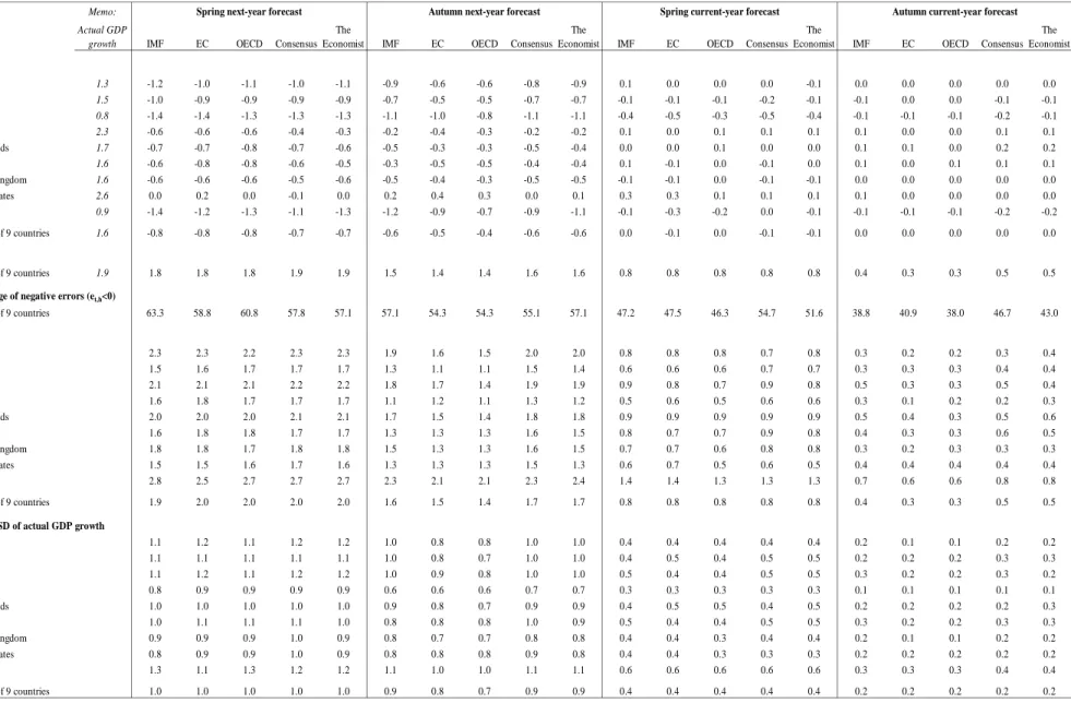
Table 1 reports some summary statistics of the projection errors. For the various countries and institutions, it is clear that accuracy improves as more relevant information becomes available to the forecaster. Both the mean forecast error and the RMSE tends to be smaller as the horizon shortens. As we would expect, this is also true for the standard deviation of forecast errors and the reduction in uncertainty seems to be especially large as we move from next-year to current-year horizons.
Regarding year-ahead horizons, the mean forecast error for the group of nine countries anal-ysed is negative for all institutions. In fact, GDP growth was overestimated more than 50 per cent of the time by all forecasters. The mean error stands at around−0.8 p.p. of GDP growth for forecasts made in Spring t−1 and around−0.5 p.p. for forecasts made in Au-tumn t−1.17 Given that actual GDP growth averaged 1.6 per cent a year over this period, the accuracy of year-ahead forecasts is not particularly impressive. The countries with larger mean errors are the three major euro area countries and Japan.18 Let’s just mention that the large negative mean error in the case of Japan is associated with a high standard deviation, as hinted from Figures 1 and 2. Regarding current-year horizons, forecasts seem to be generally unbiased. For the group of countries studied, the mean forecast error is very small and in the case of Autumn current-year forecasts is basically zero.
Looking at the RMSE adjusted by the standard deviation of GDP growth outcomes, to take
14As mentioned before, we decided to use for each institution its own outcome value (as reported in its Spring forecast exercise of the
following year) but the outcomes for each country turn out to be quite similar across institutions.
15The United States is an exception given that GDP growth seems to have been underestimated most of the time, though there was a
significant overestimation during the latest recession.
16This looks consistent with existing evidence of a considerable sluggishness in revisions of growth forecasts, as documented for
example in Loungani et al. (2011).
17If we exclude the 2009 recession, the mean error would still be negative but slightly less: around−0.5 p.p. for forecasts made in
Spring t−1 and around−0.3 p.p. for forecasts made in Autumn t−1.
into account the fact that countries with higher GDP volatility might be harder to predict, the forecasting performance becomes somewhat more similar across the various countries.
Table A.1 in the appendix indicates that the correlation of projection errors across countries is higher for year-ahead horizons but especially among euro area countries and, though less so, among these and the United Kingdom. The United States’ and Japan’s forecast errors are weakly correlated with each other and with those of other countries. Therefore, it can be said that error correlation appears to be substantial only for longer horizons and for economies with more synchronised business cycles, such as the euro area countries.
Inflation
Figures 5 to 8 show that, as in the case of GDP growth, inflation forecast errors are more significant for next-year forecasts and closer to zero for current-year forecasts (especially for Autumn current-year) across all institutions and countries. Also, projection errors are in general similar for the three institutions (IMF, Consensus and The Economist). In contrast to GDP forecasts, inflation projection errors are weakly correlated across countries, even for longer projection horizons.
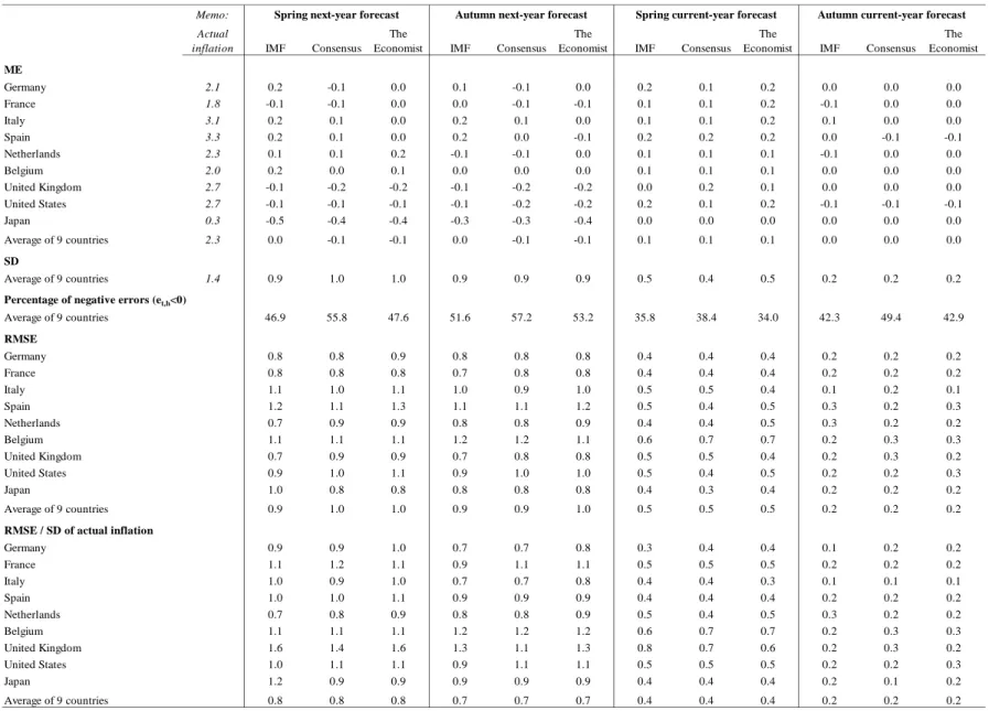
Looking at Figures 5 and 6, next-year inflation forecast errors were mostly negative (overes-timation) during the 1990’s and again during the latest recession, as forecasters were slow to anticipate the deceleration of prices during that period. Errors were, however, mostly posi-tive during the 2000’s, a period of some upturn or stabilisation of inflation in this group of countries. This explains why, in contrast to what was seen for GDP growth, the mean infla-tion forecast error for the group of nine countries is very close to zero (±0.1 p.p.) both for year-ahead and current-year horizons (Table 2).19 Japan stands out as an exception to this pattern.
According to the RMSE, the accuracy of inflation projections tends to improve as the length of the projection horizon decreases. The improvement in accuracy is much more clear as we move from next-year to current-year forecasts. Looking at the RMSE adjusted by the standard deviation of inflation outcomes we see that, for the group of nine countries, the three institutions are somewhat more accurate at predicting inflation than GDP growth for year-ahead horizons, even after taking into account the higher volatility of GDP.
3.2 Assessing relative accuracy
To judge the quality of forecasts we also want to know if they compare favorably with al-ternative forecasts that are available to users. As explained above, we examine how the
forecasts of the five institutions compare with those obtained from a naive benchmark and how do international organisations’ forecasts compare with those of private analysts. For that, we look at relative statistics of the errors of the various forecasts and test the statistical significance of the differences in accuracy among them.20
GDP growth
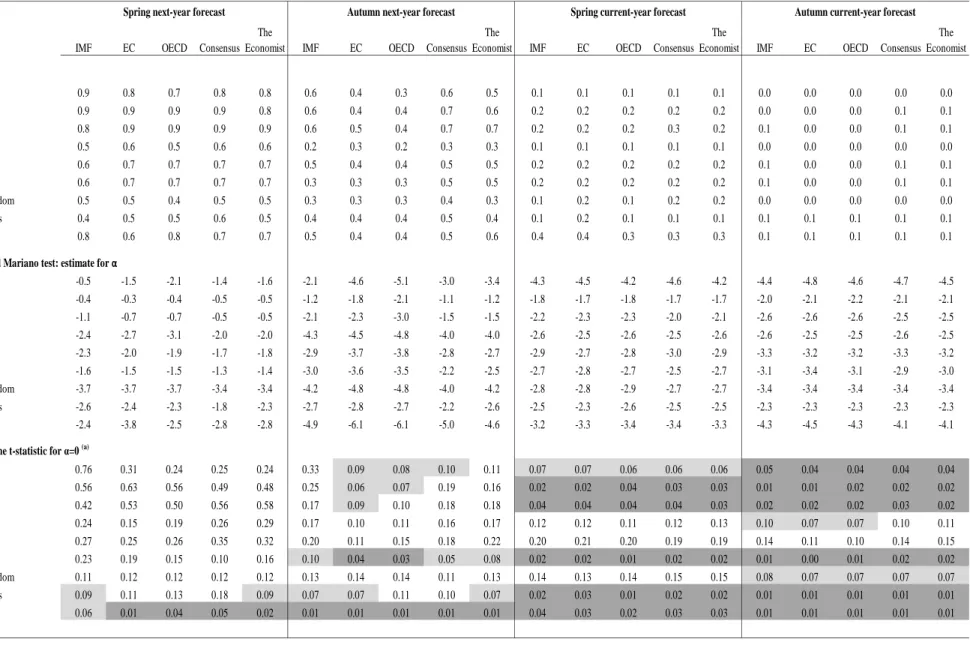
Table 3 reports Theil’s U coefficient for the comparison of the various institutions’ GDP growth forecasts with a same-change naive benchmark. All forecasters have U coefficients that are less than one, meaning that they all have a lower MSE than the naive forecast.21 However, according to the results of the test proposed by Diebold and Mariano (1995), the five forecasters are significantly better than the naive benchmark for current-year but not for next-year horizons. The negative estimate for the parameterαin all cases is the equivalent to the result of a U coefficient lower than one. For current-year horizons, we are able to reject the null hypothesis of equal forecast accuracy for most countries, at the 10 per cent significance level. For next-year horizons, it is not possible to conclude that the forecasters were significantly better than the naive for the majority of countries, with a clear exception for the case of Japan.
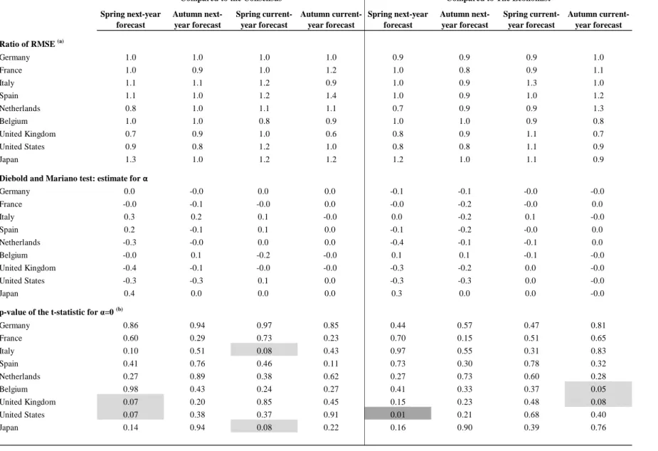
The comparison of the forecast accuracy of the three international organisations with that of the two private institutions is reported in Table 4.22 In general, the RMSE of international organisations’ forecasts does not seem to differ much from that of private analysts, for the various countries and forecasting horizons. The ratio of RMSE is in most cases close to one. The test of statistical significance of the difference between the two sets of forecasts confirms that, in general, we cannot reject the hypothesis that international organisations and private analysts have similar forecast accuracy. There are just a few cases for the shorter forecasting horizon (Autumn current-year) where this hypothesis is rejected. In most of these cases one of the international organisations, though not always the same, proved to be more accurate than the Consensus or The Economist (ratio of RMSE lower than one⇔negative estimate for the parameter α). The evidence is somewhat more consistent for the cases of France and Belgium but even for these countries it seems far-fetched to conclude that international
20It is worth mentioning that when analysing the accuracy of international organisations relative to private analysts, besides running the
Diebold and Mariano (1995) test for equal forecast accuracy, we also test for forecast encompassing. This tests if all the relevant informa-tion in private analysts’ forecasts is contained in internainforma-tional organisainforma-tions’ forecasts and vice versa. The test for forecast encompassing is implemented by running a modification of the Diebold and Mariano test as proposed in Harvey et al. (1998). However, the strong collinearity among the pairs of forecasts being tested (as already indicated by the high correlation coefficients seen in the previous subsec-tion) hampers the analysis. In various cases we can not reject encompassing in both directions, in contradiction with the very definition of encompassing. Therefore, no meaningful conclusions can be drawn.
21This same-change naive benchmark proved to be more demanding than a no-change benchmark as we expected: Theil’s U coefficients
are generally higher. There are a few exceptions for year-ahead forecasts for Germany, Italy and Japan, which experienced around zero GDP growth rates during some years of the sample.
22Recall that, as explained in section 2, each international organisation is compared with its specific data set for the Consensus and for
organisations perform consistently better in the shorter horizon.23
Inflation
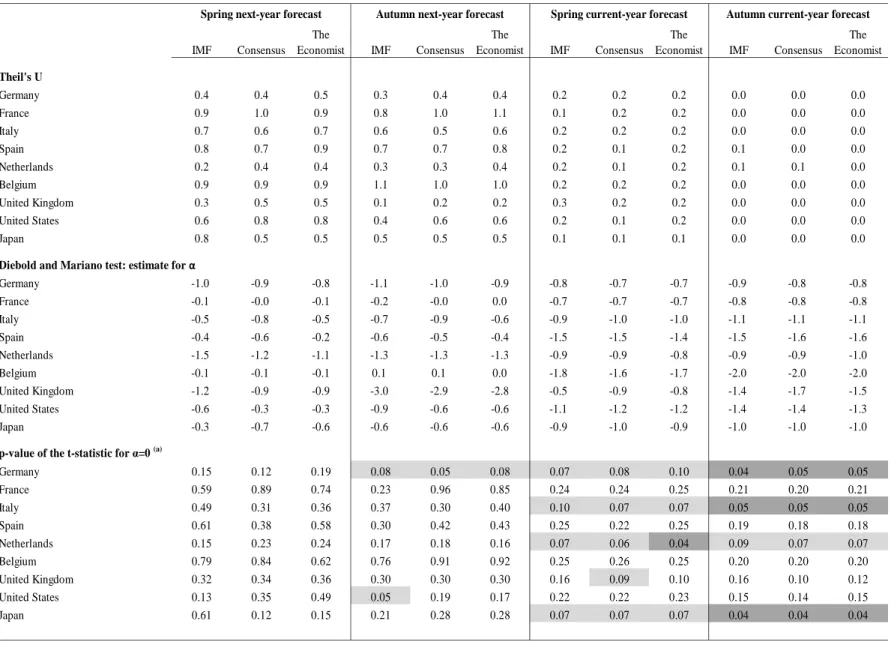
In the case of inflation, looking at Theil’s U coefficient we see that the forecasts of the three institutions have, in the majority of cases, a lower MSE than a same-change naive forecast (Table 5).24 When we test this difference for statistical significance it is not possible, in general, to reject the hypothesis that the forecasters were as accurate as this minimum standard for next-year horizons. This is not surprising given that a known result of the literature on inflation forecasting is that random walk models have proven to be surprisingly strong benchmarks in many situations (Stock and Watson (1999)). For current-year horizons, and in contrast to the case of GDP, the evidence is that the three forecasters beat the naive benchmark merely for certain economies (Germany, Italy, Netherlands and Japan).
As reported in Table 6, the quantitative accuracy of IMF’s inflation forecasts is, by and large, similar to that of Consensus or The Economist for the various horizons and economies under review.25
4
Efficiency of forecasts
The evaluation of forecasts provided in the previous section does not assess their quality in the sense of being optimal with regard to a particular information set. To assess this we need to establish testable properties that an optimal forecast should have and, for that, we will as-sume that the objective function of forecasters is of the mean squared error type, i.e. forecasts minimize a symmetric quadratic loss function. As discussed in Timmermann (2007), this im-plies, under broad conditions, that the optimal forecast is unbiased and there is absence of serial correlation in the forecast errors. The existence of serially correlated errors means that it would be possible to improve the forecast using the information on known past errors. These requirements are usually referred to in the literature as weak efficiency requirements and are empirically tested for our data set.26 It should be mentioned that a stricter condi-tion for optimal forecasts under a mean squared error loss funccondi-tion is that no variable in the current information set should be able to predict future forecast errors. No empirical test is provided for this condition given the arbitrariness of choosing each forecaster’s information set at the time of forecasting.
23We also run a Diebold and Mariano (1995) test for differences in accuracy among the international organisations and among the two
private analysts and, again, it is not possible to reject equal forecast accuracy for the vast majority of cases.
24As for GDP growth, this same-change naive benchmark proved to be in general more demanding than a no-change benchmark. 25The same conclusion applies for differences in accuracy among the two private institutions.
26Note that, as shown by Patton and Timmermann (2007), these standard optimality properties can be invalid under asymmetric loss
functions and nonlinearities (e.g. if the costs associated with over- and under-predicting a variable are not symmetric it might be optimal to bias the forecast).
The test for the weak efficiency requirements is performed directly on the properties of the forecasting errors (unbiasedness and absence of serial correlation). Indeed, for a h-period-ahead forecast to be efficient, forecast errors can follow a moving average process of order not higher than h−1.27 To implement the test we estimate the regression:
et,h=γ+βet−1,h+εt,h (7)
and perform the three following tests: a t-test forγ=0 (unbiasedness), a t-test forβ=0 (no serial correlation) and an F-test for the joint hypothesisγ =0,β=0 (weak efficiency). If βis significantly different from zero it would indicate that there is a systematic error with autocorrelation of a higher than appropriate order.
For the above econometric tests to be valid it must be the case that there is no serial correla-tion in the residual termsεt,h. The Breusch-Godfrey test is carried out to test for the presence
of serial correlation in the residuals. In cases deemed necessary, the test for weak efficiency is performed by running the alternative regression:
et,h=γ+β1et−1,h+β2et−2,h+εt,h (8)
and testing forβ1=β2=0 (no serial correlation) and forγ=β1=β2=0 (weak efficiency).
GDP growth
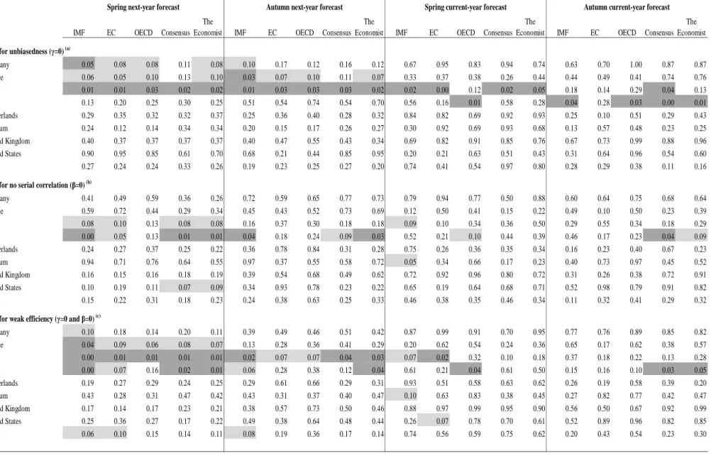
The evidence regarding unbiasedness of GDP growth forecasts, presented in Table 7,28shows that for the majority of countries we are not able to reject that the mean error of year-ahead forecasts is statistically equal to zero. However, as hinted from the analysis in section 3, forecasters present a tendency to significantly overestimate GDP growth for the major euro area countries in year-ahead horizons.29 Current-year forecasts have no significant bias for the vast majority of countries and institutions (with a few exceptions for Italy and Spain).30
When testing jointly for unbiasedness and no serial correlation of forecast errors, it is not possible in most cases to reject that forecasts are efficient for current-year horizons. For year-ahead horizons, the evidence points to inefficiency of the various institutions’ forecasts for some euro area countries. This means that projections could have been improved if either the average bias or the information contained in past errors were properly taken into account.
27Given that we are working with annual data, we assumed that h could be either equal to 1 (for current-year forecasts) or 2 (for
year-ahead forecasts). For h=1, the errors must be serially uncorrelated.
28Results presented for Germany, France, Italy and Spain refer to equation 8, given that the Breusch-Godfrey test applied to equation 7
indicated possible serial correlation of the residuals in various cases.
29The evidence of a significant bias for major euro area countries in year-ahead horizons still holds if we exclude 2009 from the sample. 30As suggested by Holden and Peel (1990), we also perform a direct test for the statistical significance of the bias by running the
regression et,h=γ+εt,hand making a simple Student’s t-test forγ=0. This test confirms in general the results presented in Table 7 but
there is additional evidence of a significant bias in year-ahead forecasts for Japan, at a 10 per cent significance level. This difference in results is probably related to the above mentioned high standard deviation of forecast errors for Japan.
Inflation
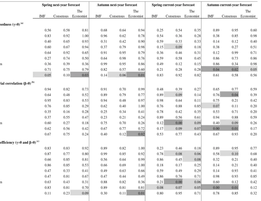
The results presented in Table 831 confirm that inflation forecasts are generally unbiased for all institutions and horizons. The next-year forecasts for Japan seem to be an exception, as al-ready mentioned in section 3. According to the formal test for weak efficiency requirements, the inflation forecasts of the three institutions can be said to be efficient in most cases, in the sense of being unbiased and of no relation between previous and current forecast errors.
5
Additional dimensions of forecast accuracy
5.1 Assessing directional accuracy
The traditional quantitative evaluation of macroeconomic forecasts tends to overlook the fact that, even if forecast errors are substantial, forecasts may provide useful information about the qualitative status of an economy, such as the acceleration/deceleration of economic activity or prices. Useful forecasts should go in the right direction. This section investigates the directional accuracy of macroeconomic forecasts, i.e. the correctness of the projected direction of change of GDP growth and inflation.
Being yt the actual growth rate in year t, let ∆yt = yt−yt−1 be the actual acceleration
(∆yt >0) or deceleration (∆yt<0) in year t. Most previous studies compute the predicted
acceleration/deceleration by comparing the forecasted growth rate with the actual growth rate of the previous period (∆byt,h=ybt,h−yt−1). However, for longer forecasting horizons
this would imply using information not yet known to forecasters at the time of forecasting. To be consistent with the approach followed in section 3 - use only information available to forecasters at each point in time - and following the methodology of Ashiya (2003), we de-cided to compute the predicted direction of change as the acceleration/deceleration implicit in the forecast at each forecasting exercise (∆bbyt,h=byt,h−ybt−1,h). To evaluate the directional
accuracy of forecasts the sign of∆bbyt,his compared to the sign of∆yt.
The directional data for each variable and country can be arranged in a 2x2 contingency table, in which the two rows represent positive and negative/null changes in the outcome and the two columns represent positive and negative/null changes in the forecast. If the number of cases in the diagonal (n11+n22 = cases where ∆yt and ∆bbyt,h are both>0 or both ≤0)
is “sufficiently ” large compared to the total number of observations (n), the forecasts are considered to be directionally accurate. More formally, we run a chi-squared independence
test as described in Carnot et al. (2005):32 2
∑
i=1 2∑
j=1 (ni j−ni.n.j/n)2 ni.n.j/n ∼χ2(1) (9)The null hypothesis is that the sign of∆ytand the sign of∆bbyt,hare independent. The rejection
of the null means that there is a significant association between the actual and the predicted direction of change and, therefore, forecasts can be said to be directionally accurate.
As before, the directional accuracy of the various forecasters is compared to that of a same-sign of change naive benchmark. This naive benchmark extrapolates the same same-sign of change for GDP growth/inflation as was last observed at the time of forecasting. Also, the forecast-ing ability of the three international organisations in terms of direction of change is compared to that of the two private sector institutions.
GDP growth
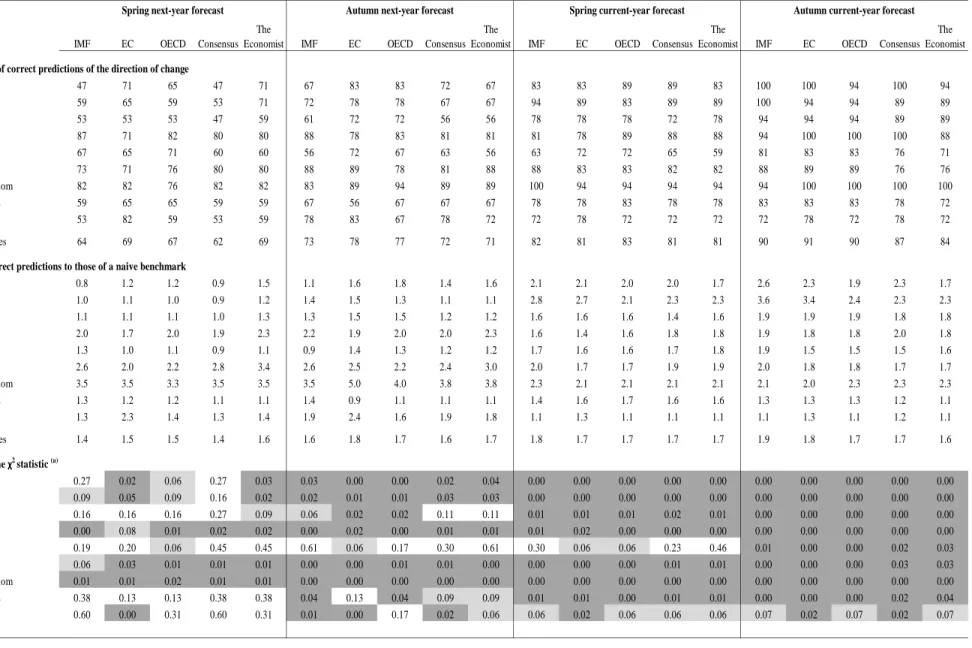
Table 9 shows the proportion of times that forecasters correctly predicted that GDP was going to accelerate or decelerate. For the group of nine countries, forecasts of all institutions are accurate more than 60/70 per cent of the time for year-ahead horizons. For current-year horizons their accuracy is higher, at around 80/90 per cent of the time.33 The results of the
chi-squared independence test for the individual countries confirm that there is a significant association between the sign of change of GDP growth in the forecasts and in the outcomes for basically all countries, with some exceptions for the longest forecasting horizon.
When looking at different benchmarks to evaluate the directional accuracy of forecasts, it is clear that the five forecasters were better at predicting the sign of change of GDP growth than a naive forecast for all horizons, even if less so for the longest one.34 When we compare the institutions among themselves,35 the directional accuracy of international organisations’ forecasts does not seem in general to differ significantly from that of the Consensus or The Economist, for the various horizons.
Inflation
Regarding inflation, forecasters correctly predicted, for current-year horizons, that consumer prices were going to accelerate or decelerate in the group of nine countries close to or more
32See Ash et al. (1998) for an application of alternative non-parametric tests on the direction of forecasts. 33Note that, for this group of countries, the sign of∆bby
t,hproved to be a more accurate predictor than the sign of∆byt,hfor year-ahead
horizons. This is in line with previous results by Ashiya (2003).
34When we apply a chi-squared independence test to the naive benchmark it is not possible in general to reject the null hypothesis of
no significant association between the actual direction of change of GDP growth and that of the naive forecast.
35Looking at the ratio of correct predictions of each international organisation to those of its corresponding data set for the Consensus
than 80 per cent of the time (Table 10). However, for year-ahead horizons they were not so well succeeded (percentage of correct predictions at around 65 per cent).36 According to the results of the non-parametric test, current-year forecasts are in general directionally accurate but for year-ahead forecasts the null hypothesis of independence between the predicted and the actual sign of inflation change can not be rejected for most countries. Note also that the ability of these forecasters to predict increases or decreases in inflation does not seem to be very different from their ability to predict accelerations or decelerations of the economic activity, even if slightly lower in a few cases.
Similar to results for GDP, the three forecasters proved to be in general more accurate at predicting the sign of change in inflation than a naive forecast. Also, the directional accuracy of IMF’s inflation forecasts can not be said to be much different from that of Consensus or The Economist.
5.2 Ability to forecast recessions
An additional informative criteria to evaluate macroeconomic forecasts is the ability to pre-dict turning points, considering both the number of actual turns that are correctly prepre-dicted and the number of false turns that are predicted. Given the limited number of changes from positive to negative growth rates or vice versa in our sample, especially in the case of infla-tion data, it was decided to limit the analysis to the forecasters ability to predict economic recessions.37 Recessions in this study are defined as any year in which real GDP declined (yt<0).
Over the sample period 1991-2009, a total of twenty-three recession episodes were identified for the group of nine countries under analysis.38 The properties of forecasts during those recession episodes are presented in Table 11. When we compute the percentage of episodes that forecasters were able to anticipate, we see that in general they are not able to anticipate in the preceding year that a recession is going to occur. This is particularly true as of Spring of the previous year and more evident in the case of private analysts. Forecasters seem to identify recessions just in the year in which they occur, though by Spring of that year around half of the recession episodes are still not acknowledged by most forecasters. By Autumn of the year of the recession, even though the decline in GDP is correctly identified in the vast majority of cases, the magnitude of the fall is still under-predicted for around 50 per cent of the cases.39
36As seen in the case of GDP growth, the predicted direction of change as computed in this work showed to be better for year-ahead
horizons than the usual alternative.
37A similar analysis of Consensus’ forecasts for a large group of countries can be found in Loungani (2001). 38Note that at the individual country level there are 2 or 3 recession episodes during the sample period.
39As mentioned in section 3, forecasters show a tendency to overestimate growth when the economy is slowing down and this is
During the period analysed, forecasters predicted a couple of false recessions, in the cases of Italy, Netherlands and Japan. This is however a rare event and in most cases happened in current-year forecasts for years with close to zero GDP growth outcomes.
The evidence on the difficulties that forecasters experience in identifying economic reces-sions in advance (or even when they are occurring) is notable, both for international organ-isations and private analysts. Though the reasons for this do not seem to have been yet adequately explored, some authors such as Loungani (2001) have suggested that either fore-casters lack the required information (reliable real-time data or models) or lack the incentives to predict recessions. In any case, we should keep in mind that these point forecasts reported by the various institutions may not capture shifts in the probability that they attach to worst case scenarios.
6
General summary and comparison with previous evaluations
In this paper, we assessed the accuracy of the IMF’s, the EC’s and the OECD’s forecasts and compared it with that of the Consensus’ and The Economist’s surveys of private an-alysts. The focus was on forecasts for economic growth and consumer price inflation for nine advanced economies, over the past two decades. We now provide an overall picture of our findings and briefly compare them with previous results from in-house evaluations of international organisations’ forecasts.
In the case of real GDP growth, we find that the accuracy of projections clearly increases as the forecast horizon shortens and more information becomes available to the forecaster. Regarding year-ahead horizons, even though it is not possible to reject that the projections of the various forecasters are unbiased and efficient in most cases, there is evidence of in-efficiency for some euro area countries. Year-ahead forecasts show a significant negative bias for major euro area countries. This appears to stem from a tendency of the various forecasters to persistently over-predict growth when the economy is slowing down and most noticeably during periods of economic recession. Also, there is tentative evidence of a high correlation of year-ahead projection errors for the euro area economies. Current-year GDP growth forecasts are generally unbiased and efficient.
Our analysis suggests that the quantitative accuracy of the GDP growth forecasts published by the IMF, the EC and the OECD is not statistically different from that of the Consensus or The Economist, for the various countries and horizons examined. In the rare exceptions observed for the shorter horizon (Autumn current-year) no institution proved to perform consistently better, even if in most cases one of the international organisations was more accurate than the Consensus or The Economist. All five forecasters beat a naive model that
projects a GDP growth rate equal to the last one observed at the time of forecasting, for current-year horizons. For year-ahead horizons, they are not in general significantly better than the naive.
Notwithstanding a few distinctive features of the analysis undertaken in this work - namely the inclusion of the most recent vintages of projections up to 2009, the assessment of a less publicised survey of private forecasters (The Economist) and the use of a slightly different empirical approach for choosing the timing of comparison of forecasts - along with some constraints coming from the relatively small sample size, our findings can be said to be broadly in line with those of the latest in-house assessments of forecasts published by the IMF, the EC and the OECD.40
Timmermann (2007) analysis of the IMF’s forecasts, over the period 1990-2003, finds that GDP growth forecasts display a tendency for over-prediction in next-year horizons for vari-ous advanced economies. However, there is very little evidence on biases or serial correlation of errors for current-year forecasts. The comparison of the IMF’s forecasts for the G7 coun-tries with those of the Consensus suggests that the performance is overall statistically similar, even if the IMF performs slightly better in a few cases for current-year horizons. The author presents some evidence that results might however be sensible to the timing of comparison. According to Melander et al. (2007) assessment of the EC’s forecasts, for the period 1969-2005, growth forecasts for the European Union generally proved to be unbiased and efficient, though there is evidence of the contrary for some Member States (e.g. an overestimation in the case of Italy). They also concluded that the track record of the EC’s forecasts for GDP growth is broadly comparable with the ones of the Consensus, the IMF and the OECD. The review of the OECD’s growth projections for the G7 countries over the period 1991-2006, carried out by Vogel (2007), found that year-ahead forecasts are less accurate and have a tendency to overestimate the outcome. Current-year projections are, however, unbiased and efficient. The author argues that the OECD’s forecasts tend to outperform the Consensus for the current-year horizon.
Regarding the directional accuracy of GDP growth forecasts, we find that the percentage of correct predictions is practically always above 50 per cent though, for all forecasters, the success rate is clearly higher for current-year horizons (at around 80/90 per cent). Although this is not always the case in the Spring next-year forecasts, for the remaining horizons there is a significant association between the direction of change of GDP growth in the forecasts and in the outcomes for basically all countries. As before, the directional accuracy of inter-national organisations’ forecasts does not seem to differ much from that of private analysts. The five forecasters are better at forecasting accelerations/decelerations of economic activity than a naive benchmark.
One result about which there is general agreement in the literature on forecasting turning points is that most forecasters fail to predict economic recessions in advance and, sometimes, fail to detect them contemporaneously.41 Notwithstanding the limited number of observa-tions, our brief evaluation of the recession episodes occurred in the sample of nine countries during the period 1991-2009 is totally consistent with this finding. As of Spring of the pre-vious year no forecaster is able to predict that GDP is going to fall and by Spring of the recession year around half of the recession episodes is still not acknowledged by most fore-casters. Moreover, the forecasts made in Autumn of the recession year still underestimate its magnitude in around 50 per cent of the cases. This underestimation was particularly no-torious during the latest economic recession for all five forecasters. Also, forecasters make very few predictions of recessions that do not occur. As pointed out by McNees (1992), this disturbing evidence about the inability to forecast economic recessions advises the forecast user not to ignore the forecasts but rather to think carefully about plausible outcomes far from the central scenarios.
Turning to inflation, recall that due to data availability the assessment only covers three fore-casters: the IMF and the two surveys of private analysts. We find that the accuracy of Spring and Autumn next-year forecasts is quite similar but it improves significantly as we move to current-year forecasts. In contrast to results seen for GDP, inflation projections are in most cases unbiased and efficient, both for year-ahead and current-year horizons. Notwith-standing, the various forecasters display some tendency to over-predict inflation when it is declining and under-predict it when it is rising. Inflation projection errors are in general weakly correlated across countries. Let’s also mention that, after taking into account that variables with higher volatility are probably harder to predict, these three forecasters seem to be slightly more accurate on average at predicting year inflation than at predicting next-year economic growth. The accuracy of inflation and GDP growth current-next-year forecasts is however quite similar.
By and large, the quantitative accuracy of the IMF’s inflation forecasts is similar to that of the Consensus or The Economist. The accuracy of these three forecasters is not in general statistically different from that of a naive random-walk model (which predicts a similar infla-tion to the last one observed) for year-ahead horizons. For current-year horizons, and unlike seen for GDP growth forecasts, they just beat the naive benchmark for a few countries.
These results do not differ much from those obtained by Timmermann (2007). According to his evaluation, the IMF’s inflation forecasts for the advanced economies are generally unbi-ased and efficient, even though he found evidence in a few cases of some under-prediction of inflation and serial correlation of forecast errors for year-ahead horizons. His results also
41See Fildes and Stekler (2002) for a survey and Loungani (2001) for evidence across a large sample of industrialised and developing
suggest that the performance of the IMF’s inflation forecasts for the G7 countries is similar to that of the Consensus.
Inflation forecasts are in general directionally accurate for current-year but not for year-ahead horizons. For current-year horizons, the three forecasters correctly predict that consumer prices are going to accelerate or decelerate close to or more than 80 per cent of the time. Similar to results for GDP, the directional accuracy of the IMF’s forecasts does not seem to differ much from that of private analysts and they are all in general more accurate at predicting the sign of inflation change than a naive benchmark.
Reassessments of the quality of macroeconomic projections are warranted from time to time, as new vintages of projections become available and new business cycle fluctuations take place. The findings of this work are in line with previous evidence that current-year fore-casts for economic growth and inflation in advanced economies present in general desirable features but year-ahead forecasts present a more mixed picture in terms of quantitative and qualitative accuracy. This understanding of how large forecast errors are likely to be and how often forecasters are likely to miss the direction where the economy is going is abso-lutely necessary in order to assess the usefulness of forecasts to its users. Some may consider disappointing the fact that the forecast performance of reputed international organisations is generally similar to that of panels of private analysts. Though we could not substantiate a consistent superior performance, we must emphasize that international organisations’ fore-casts serve a quite different purpose from those of private institutions. They do provide more than just point forecasts. In particular, they provide a detailed and consistent picture for the international outlook and a thorough discussion of the main issues and risks, besides policy recommendations potentially valuable to policymakers. For the forecast user it might how-ever be comforting to learn that he can place as much (little) confidence in the alternative private analysts’ forecasts that are available on a monthly basis. In further work, it might be interesting to explore possible uses of private analysts’ forecasts which become available in-between disclosures of a new forecast exercise by international organisations.
References
Artis, M. J. (1997), How accurate are the IMF’s short-term forecasts? Another examination of the World Economic Outlook, Staff Studies for the World Economic Outlook - World Economic and Financial Surveys, International Monetary Fund.
Ash, J. C. K., Smyth, D. J. and Heravi, S. M. (1998), ‘Are OECD forecasts rational and useful?: a directional analysis’, International Journal of Forecasting 14(3), 381–391.
Ashiya, M. (2003), ‘The directional accuracy of 15-months-ahead forecasts made by the IMF’, Applied Economics Letters 10(6), 331–333.
Carnot, N., Koen, V. and Tissot, B. (2005), Economic Forecasting, Palgrave MacMillan.
Diebold, F. X. and Mariano, R. S. (1995), ‘Comparing predictive accuracy’, Journal of Busi-ness and Economic Statistics 13(3), 253–263.
Fildes, R. and Stekler, H. (2002), ‘The state of macroeconomic forecasting’, Journal of Macroeconomics 24(4), 435–468.
Harvey, D., Leybourne, S. and Newbold, P. (1997), ‘Testing the equality of prediction mean squared errors’, International Journal of Forecasting 13(2), 281–291.
Harvey, D., Leybourne, S. and Newbold, P. (1998), ‘Tests for forecast encompassing’, Jour-nal of Business and Economic Statistics 16(2), 254–259.
Holden, K. and Peel, D. A. (1990), ‘On testing for unbiasedness and efficiency of forecasts’, The Manchester School 58(2), 120–127.
Keereman, F. (1999), The track record of the Commission forecasts, Economic Papers 137, European Commission (Directorate General for Economic and Financial Affairs).
Koutsogeorgopoulou, V. (2000), A post-mortem on Economic Outlook projections, OECD Economics Department Working Papers 274, OECD.
Lenain, P. (2001), What is the track record of OECD economic projections?, Technical re-port, OECD Economics Department.
Loungani, P. (2001), ‘How accurate are private sector forecasts? Cross-country
evi-dence from consensus forecasts of output growth’, International Journal of Forecasting
17(3), 419–432.
Loungani, P., Stekler, H. and Tamirisa, N. (2011), Information rigidity in growth forecasts: Some cross-country evidence, IMF Working Paper 125, International Monetary Fund.
McNees, S. (1992), ‘How large are economic forecast errors?’, New England Economic Review pp. 25–42.
Melander, A., Sismanidis, G. and Grenouilleau, D. (2007), The track record of the Com-mission’s forecasts - an update, Economic Papers 291, European Commission (Directorate General for Economic and Financial Affairs).
Patton, A. J. and Timmermann, A. (2007), ‘Properties of optimal forecasts under asymmetric loss and nonlinearity’, Journal of Econometrics 140(2), 884 – 918.
Stock, J. H. and Watson, M. W. (1999), ‘Forecasting inflation’, Journal of Monetary Eco-nomics 44(2), 293–335.
Theil, H. (1971), Applied Economic Forecasting, North-Holland Publishing Company.
Timmermann, A. (2007), ‘An evaluation of the World Economic Outlook forecasts’, IMF Staff Papers 54(1), 1–33.
Vogel, L. (2007), How do the OECD growth projections for the G7 economies perform? A post-mortem, OECD Economics Department Working Papers 573, OECD.
Vuchelen, J. and Gutierrez, M.-I. (2005), ‘Do the OECD 24 month horizon growth forecasts for the G7-countries contain information?’, Applied Economics 37(8), 855–862.
Zarnowitz, V. and Braun, P. A. (1993), Twenty-two years of the NBER-ASA quarterly eco-nomic outlook surveys: Aspects and comparisons of forecasting performance, in J. Stock and M. Watson, eds, ‘Business Cycles, Indicators and Forecasting’, The University of Chicago Press, pp. 11–93.
Table 1: Descriptive statistics of GDP growth forecast errors (1991-2009) Memo:
Actual GDP
growth IMF EC OECD Consensus The
Economist IMF EC OECD Consensus The
Economist IMF EC OECD Consensus The
Economist IMF EC OECD Consensus The Economist ME Germany 1.3 -1.2 -1.0 -1.1 -1.0 -1.1 -0.9 -0.6 -0.6 -0.8 -0.9 0.1 0.0 0.0 0.0 -0.1 0.0 0.0 0.0 0.0 0.0 France 1.5 -1.0 -0.9 -0.9 -0.9 -0.9 -0.7 -0.5 -0.5 -0.7 -0.7 -0.1 -0.1 -0.1 -0.2 -0.1 -0.1 0.0 0.0 -0.1 -0.1 Italy 0.8 -1.4 -1.4 -1.3 -1.3 -1.3 -1.1 -1.0 -0.8 -1.1 -1.1 -0.4 -0.5 -0.3 -0.5 -0.4 -0.1 -0.1 -0.1 -0.2 -0.1 Spain 2.3 -0.6 -0.6 -0.6 -0.4 -0.3 -0.2 -0.4 -0.3 -0.2 -0.2 0.1 0.0 0.1 0.1 0.1 0.1 0.0 0.0 0.1 0.1 Netherlands 1.7 -0.7 -0.7 -0.8 -0.7 -0.6 -0.5 -0.3 -0.3 -0.5 -0.4 0.0 0.0 0.1 0.0 0.0 0.1 0.1 0.0 0.2 0.2 Belgium 1.6 -0.6 -0.8 -0.8 -0.6 -0.5 -0.3 -0.5 -0.5 -0.4 -0.4 0.1 -0.1 0.0 -0.1 0.0 0.1 0.0 0.1 0.1 0.1 United Kingdom 1.6 -0.6 -0.6 -0.6 -0.5 -0.6 -0.5 -0.4 -0.3 -0.5 -0.5 -0.1 -0.1 0.0 -0.1 -0.1 0.0 0.0 0.0 0.0 0.0 United States 2.6 0.0 0.2 0.0 -0.1 0.0 0.2 0.4 0.3 0.0 0.1 0.3 0.3 0.1 0.1 0.1 0.1 0.0 0.0 0.0 0.0 Japan 0.9 -1.4 -1.2 -1.3 -1.1 -1.3 -1.2 -0.9 -0.7 -0.9 -1.1 -0.1 -0.3 -0.2 0.0 -0.1 -0.1 -0.1 -0.1 -0.2 -0.2 Average of 9 countries 1.6 -0.8 -0.8 -0.8 -0.7 -0.7 -0.6 -0.5 -0.4 -0.6 -0.6 0.0 -0.1 0.0 -0.1 -0.1 0.0 0.0 0.0 0.0 0.0 SD Average of 9 countries 1.9 1.8 1.8 1.8 1.9 1.9 1.5 1.4 1.4 1.6 1.6 0.8 0.8 0.8 0.8 0.8 0.4 0.3 0.3 0.5 0.5
Percentage of negative errors (et,h<0)
Average of 9 countries 63.3 58.8 60.8 57.8 57.1 57.1 54.3 54.3 55.1 57.1 47.2 47.5 46.3 54.7 51.6 38.8 40.9 38.0 46.7 43.0 RMSE Germany 2.3 2.3 2.2 2.3 2.3 1.9 1.6 1.5 2.0 2.0 0.8 0.8 0.8 0.7 0.8 0.3 0.2 0.2 0.3 0.4 France 1.5 1.6 1.7 1.7 1.7 1.3 1.1 1.1 1.5 1.4 0.6 0.6 0.6 0.7 0.7 0.3 0.3 0.3 0.4 0.4 Italy 2.1 2.1 2.1 2.2 2.2 1.8 1.7 1.4 1.9 1.9 0.9 0.8 0.7 0.9 0.8 0.5 0.3 0.3 0.5 0.4 Spain 1.6 1.8 1.7 1.7 1.7 1.1 1.2 1.1 1.3 1.2 0.5 0.6 0.5 0.6 0.6 0.3 0.1 0.2 0.2 0.3 Netherlands 2.0 2.0 2.0 2.1 2.1 1.7 1.5 1.4 1.8 1.8 0.9 0.9 0.9 0.9 0.9 0.5 0.4 0.3 0.5 0.6 Belgium 1.6 1.8 1.8 1.7 1.7 1.3 1.3 1.3 1.6 1.5 0.8 0.7 0.7 0.9 0.8 0.4 0.3 0.3 0.6 0.5 United Kingdom 1.8 1.8 1.7 1.8 1.8 1.5 1.3 1.3 1.6 1.5 0.7 0.7 0.6 0.8 0.8 0.3 0.2 0.3 0.3 0.3 United States 1.5 1.5 1.6 1.7 1.6 1.3 1.3 1.3 1.5 1.3 0.6 0.7 0.5 0.6 0.5 0.4 0.4 0.4 0.4 0.4 Japan 2.8 2.5 2.7 2.7 2.7 2.3 2.1 2.1 2.3 2.4 1.4 1.4 1.3 1.3 1.3 0.7 0.6 0.6 0.8 0.8 Average of 9 countries 1.9 2.0 2.0 2.0 2.0 1.6 1.5 1.4 1.7 1.7 0.8 0.8 0.8 0.8 0.8 0.4 0.3 0.3 0.5 0.5
RMSE / SD of actual GDP growth
Germany 1.1 1.2 1.1 1.2 1.2 1.0 0.8 0.8 1.0 1.0 0.4 0.4 0.4 0.4 0.4 0.2 0.1 0.1 0.2 0.2 France 1.1 1.1 1.1 1.1 1.1 1.0 0.8 0.7 1.0 1.0 0.4 0.5 0.4 0.5 0.5 0.2 0.2 0.2 0.3 0.3 Italy 1.1 1.2 1.1 1.2 1.2 1.0 0.9 0.8 1.0 1.0 0.5 0.4 0.4 0.5 0.5 0.3 0.2 0.2 0.3 0.2 Spain 0.8 0.9 0.9 0.9 0.9 0.6 0.6 0.6 0.7 0.7 0.3 0.3 0.3 0.3 0.3 0.1 0.1 0.1 0.1 0.1 Netherlands 1.0 1.0 1.0 1.0 1.0 0.9 0.8 0.7 0.9 0.9 0.4 0.5 0.5 0.4 0.5 0.2 0.2 0.2 0.2 0.3 Belgium 1.0 1.1 1.1 1.1 1.0 0.8 0.8 0.8 1.0 0.9 0.5 0.4 0.4 0.5 0.5 0.3 0.2 0.2 0.3 0.3 United Kingdom 0.9 0.9 0.9 1.0 0.9 0.8 0.7 0.7 0.8 0.8 0.4 0.4 0.3 0.4 0.4 0.2 0.1 0.1 0.2 0.2 United States 0.8 0.9 0.9 1.0 0.9 0.8 0.8 0.8 0.9 0.8 0.4 0.4 0.3 0.3 0.3 0.2 0.2 0.2 0.2 0.2 Japan 1.3 1.1 1.3 1.2 1.2 1.1 1.0 1.0 1.1 1.1 0.6 0.6 0.6 0.6 0.6 0.3 0.3 0.3 0.4 0.4 Average of 9 countries 1.0 1.0 1.0 1.0 1.0 0.9 0.8 0.7 0.9 0.9 0.4 0.4 0.4 0.4 0.4 0.2 0.2 0.2 0.2 0.2
Spring next-year forecast Autumn next-year forecast Spring current-year forecast Autumn current-year forecast
Sources: IMF, EC, OECD, Consensus Economics, The Economist and author’s calculations.
2
Table 2: Descriptive statistics of inflation forecast errors (1991-2009)
Memo: Actual
inflation IMF Consensus The
Economist IMF Consensus The
Economist IMF Consensus The
Economist IMF Consensus The Economist ME Germany 2.1 0.2 -0.1 0.0 0.1 -0.1 0.0 0.2 0.1 0.2 0.0 0.0 0.0 France 1.8 -0.1 -0.1 0.0 0.0 -0.1 -0.1 0.1 0.1 0.2 -0.1 0.0 0.0 Italy 3.1 0.2 0.1 0.0 0.2 0.1 0.0 0.1 0.1 0.2 0.1 0.0 0.0 Spain 3.3 0.2 0.1 0.0 0.2 0.0 -0.1 0.2 0.2 0.2 0.0 -0.1 -0.1 Netherlands 2.3 0.1 0.1 0.2 -0.1 -0.1 0.0 0.1 0.1 0.1 -0.1 0.0 0.0 Belgium 2.0 0.2 0.0 0.1 0.0 0.0 0.0 0.1 0.1 0.1 0.0 0.0 0.0 United Kingdom 2.7 -0.1 -0.2 -0.2 -0.1 -0.2 -0.2 0.0 0.2 0.1 0.0 0.0 0.0 United States 2.7 -0.1 -0.1 -0.1 -0.1 -0.2 -0.2 0.2 0.1 0.2 -0.1 -0.1 -0.1 Japan 0.3 -0.5 -0.4 -0.4 -0.3 -0.3 -0.4 0.0 0.0 0.0 0.0 0.0 0.0 Average of 9 countries 2.3 0.0 -0.1 -0.1 0.0 -0.1 -0.1 0.1 0.1 0.1 0.0 0.0 0.0 SD Average of 9 countries 1.4 0.9 1.0 1.0 0.9 0.9 0.9 0.5 0.4 0.5 0.2 0.2 0.2
Percentage of negative errors (et,h<0)
Average of 9 countries 46.9 55.8 47.6 51.6 57.2 53.2 35.8 38.4 34.0 42.3 49.4 42.9 RMSE Germany 0.8 0.8 0.9 0.8 0.8 0.8 0.4 0.4 0.4 0.2 0.2 0.2 France 0.8 0.8 0.8 0.7 0.8 0.8 0.4 0.4 0.4 0.2 0.2 0.2 Italy 1.1 1.0 1.1 1.0 0.9 1.0 0.5 0.5 0.4 0.1 0.2 0.1 Spain 1.2 1.1 1.3 1.1 1.1 1.2 0.5 0.4 0.5 0.3 0.2 0.3 Netherlands 0.7 0.9 0.9 0.8 0.8 0.9 0.4 0.4 0.5 0.3 0.2 0.2 Belgium 1.1 1.1 1.1 1.2 1.2 1.1 0.6 0.7 0.7 0.2 0.3 0.3 United Kingdom 0.7 0.9 0.9 0.7 0.8 0.8 0.5 0.5 0.4 0.2 0.3 0.2 United States 0.9 1.0 1.1 0.9 1.0 1.0 0.5 0.4 0.5 0.2 0.2 0.3 Japan 1.0 0.8 0.8 0.8 0.8 0.8 0.4 0.3 0.4 0.2 0.2 0.2 Average of 9 countries 0.9 1.0 1.0 0.9 0.9 1.0 0.5 0.5 0.5 0.2 0.2 0.2
RMSE / SD of actual inflation
Germany 0.9 0.9 1.0 0.7 0.7 0.8 0.3 0.4 0.4 0.1 0.2 0.2 France 1.1 1.2 1.1 0.9 1.1 1.1 0.5 0.5 0.5 0.2 0.2 0.2 Italy 1.0 0.9 1.0 0.7 0.7 0.8 0.4 0.4 0.3 0.1 0.1 0.1 Spain 1.0 1.0 1.1 0.9 0.9 0.9 0.4 0.4 0.4 0.2 0.2 0.2 Netherlands 0.7 0.8 0.9 0.8 0.8 0.9 0.5 0.4 0.5 0.3 0.2 0.2 Belgium 1.1 1.1 1.1 1.2 1.2 1.2 0.6 0.7 0.7 0.2 0.3 0.3 United Kingdom 1.6 1.4 1.6 1.3 1.1 1.3 0.8 0.7 0.6 0.2 0.3 0.2 United States 1.0 1.1 1.1 0.9 1.1 1.1 0.5 0.5 0.5 0.2 0.2 0.3 Japan 1.2 0.9 0.9 0.9 0.9 0.9 0.4 0.4 0.4 0.2 0.1 0.2 Average of 9 countries 0.8 0.8 0.8 0.7 0.7 0.7 0.4 0.4 0.4 0.2 0.2 0.2
Spring next-year forecast Autumn next-year forecast Spring current-year forecast Autumn current-year forecast
Sources: IMF, Consensus Economics, The Economist and author’s calculations.
2
Table 3: GDP growth - Comparison of the forecast accuracy of each institution with that of a same-change naive forecast
IMF EC OECD Consensus
The
Economist IMF EC OECD Consensus
The
Economist IMF EC OECD Consensus
The
Economist IMF EC OECD Consensus
The Economist Theil's U Germany 0.9 0.8 0.7 0.8 0.8 0.6 0.4 0.3 0.6 0.5 0.1 0.1 0.1 0.1 0.1 0.0 0.0 0.0 0.0 0.0 France 0.9 0.9 0.9 0.9 0.8 0.6 0.4 0.4 0.7 0.6 0.2 0.2 0.2 0.2 0.2 0.0 0.0 0.0 0.1 0.1 Italy 0.8 0.9 0.9 0.9 0.9 0.6 0.5 0.4 0.7 0.7 0.2 0.2 0.2 0.3 0.2 0.1 0.0 0.0 0.1 0.1 Spain 0.5 0.6 0.5 0.6 0.6 0.2 0.3 0.2 0.3 0.3 0.1 0.1 0.1 0.1 0.1 0.0 0.0 0.0 0.0 0.0 Netherlands 0.6 0.7 0.7 0.7 0.7 0.5 0.4 0.4 0.5 0.5 0.2 0.2 0.2 0.2 0.2 0.1 0.0 0.0 0.1 0.1 Belgium 0.6 0.7 0.7 0.7 0.7 0.3 0.3 0.3 0.5 0.5 0.2 0.2 0.2 0.2 0.2 0.1 0.0 0.0 0.1 0.1 United Kingdom 0.5 0.5 0.4 0.5 0.5 0.3 0.3 0.3 0.4 0.3 0.1 0.2 0.1 0.2 0.2 0.0 0.0 0.0 0.0 0.0 United States 0.4 0.5 0.5 0.6 0.5 0.4 0.4 0.4 0.5 0.4 0.1 0.2 0.1 0.1 0.1 0.1 0.1 0.1 0.1 0.1 Japan 0.8 0.6 0.8 0.7 0.7 0.5 0.4 0.4 0.5 0.6 0.4 0.4 0.3 0.3 0.3 0.1 0.1 0.1 0.1 0.1
Diebold and Mariano test: estimate for α
Germany -0.5 -1.5 -2.1 -1.4 -1.6 -2.1 -4.6 -5.1 -3.0 -3.4 -4.3 -4.5 -4.2 -4.6 -4.2 -4.4 -4.8 -4.6 -4.7 -4.5 France -0.4 -0.3 -0.4 -0.5 -0.5 -1.2 -1.8 -2.1 -1.1 -1.2 -1.8 -1.7 -1.8 -1.7 -1.7 -2.0 -2.1 -2.2 -2.1 -2.1 Italy -1.1 -0.7 -0.7 -0.5 -0.5 -2.1 -2.3 -3.0 -1.5 -1.5 -2.2 -2.3 -2.3 -2.0 -2.1 -2.6 -2.6 -2.6 -2.5 -2.5 Spain -2.4 -2.7 -3.1 -2.0 -2.0 -4.3 -4.5 -4.8 -4.0 -4.0 -2.6 -2.5 -2.6 -2.5 -2.6 -2.6 -2.5 -2.5 -2.6 -2.5 Netherlands -2.3 -2.0 -1.9 -1.7 -1.8 -2.9 -3.7 -3.8 -2.8 -2.7 -2.9 -2.7 -2.8 -3.0 -2.9 -3.3 -3.2 -3.2 -3.3 -3.2 Belgium -1.6 -1.5 -1.5 -1.3 -1.4 -3.0 -3.6 -3.5 -2.2 -2.5 -2.7 -2.8 -2.7 -2.5 -2.7 -3.1 -3.4 -3.1 -2.9 -3.0 United Kingdom -3.7 -3.7 -3.7 -3.4 -3.4 -4.2 -4.8 -4.8 -4.0 -4.2 -2.8 -2.8 -2.9 -2.7 -2.7 -3.4 -3.4 -3.4 -3.4 -3.4 United States -2.6 -2.4 -2.3 -1.8 -2.3 -2.7 -2.8 -2.7 -2.2 -2.6 -2.5 -2.3 -2.6 -2.5 -2.5 -2.3 -2.3 -2.3 -2.3 -2.3 Japan -2.4 -3.8 -2.5 -2.8 -2.8 -4.9 -6.1 -6.1 -5.0 -4.6 -3.2 -3.3 -3.4 -3.4 -3.3 -4.3 -4.5 -4.3 -4.1 -4.1
p-value of the t-statistic for α=0 (a)
Germany 0.76 0.31 0.24 0.25 0.24 0.33 0.09 0.08 0.10 0.11 0.07 0.07 0.06 0.06 0.06 0.05 0.04 0.04 0.04 0.04 France 0.56 0.63 0.56 0.49 0.48 0.25 0.06 0.07 0.19 0.16 0.02 0.02 0.04 0.03 0.03 0.01 0.01 0.02 0.02 0.02 Italy 0.42 0.53 0.50 0.56 0.58 0.17 0.09 0.10 0.18 0.18 0.04 0.04 0.04 0.04 0.03 0.02 0.02 0.02 0.03 0.02 Spain 0.24 0.15 0.19 0.26 0.29 0.17 0.10 0.11 0.16 0.17 0.12 0.12 0.11 0.12 0.13 0.10 0.07 0.07 0.10 0.11 Netherlands 0.27 0.25 0.26 0.35 0.32 0.20 0.11 0.15 0.18 0.22 0.20 0.21 0.20 0.19 0.19 0.14 0.11 0.10 0.14 0.15 Belgium 0.23 0.19 0.15 0.10 0.16 0.10 0.04 0.03 0.05 0.08 0.02 0.02 0.01 0.02 0.02 0.01 0.00 0.01 0.02 0.02 United Kingdom 0.11 0.12 0.12 0.12 0.12 0.13 0.14 0.14 0.11 0.13 0.14 0.13 0.14 0.15 0.15 0.08 0.07 0.07 0.07 0.07 United States 0.09 0.11 0.13 0.18 0.09 0.07 0.07 0.11 0.10 0.07 0.02 0.03 0.01 0.02 0.02 0.01 0.01 0.01 0.01 0.01 Japan 0.06 0.01 0.04 0.05 0.02 0.01 0.01 0.01 0.01 0.01 0.04 0.03 0.02 0.03 0.03 0.01 0.01 0.01 0.01 0.01
Spring next-year forecast Autumn next-year forecast Spring current-year forecast Autumn current-year forecast
Sources: IMF, EC, OECD, Consensus Economics, The Economist and author’s calculations. Note:
2