University of Central Florida University of Central Florida
STARS
STARS
Electronic Theses and Dissertations, 2004-20192006
Algorithms For Discovering Communities In Complex Networks
Algorithms For Discovering Communities In Complex Networks
Hemant BalakrishnanUniversity of Central Florida
Part of the Computer Sciences Commons, and the Engineering Commons Find similar works at: https://stars.library.ucf.edu/etd
University of Central Florida Libraries http://library.ucf.edu
This Doctoral Dissertation (Open Access) is brought to you for free and open access by STARS. It has been accepted for inclusion in Electronic Theses and Dissertations, 2004-2019 by an authorized administrator of STARS. For more information, please contact [email protected].
STARS Citation STARS Citation
Balakrishnan, Hemant, "Algorithms For Discovering Communities In Complex Networks" (2006). Electronic Theses and Dissertations, 2004-2019. 1102.
ALGORITHMS FOR DISCOVERING COMMUNITIES IN COMPLEX NETWORKS
by
HEMANT BALAKRISHNAN B.E. Bharathiar University, 2000 M.S. University of Texas at Dallas, 2002
A dissertation submitted in partial fulfillment of the requirements for the degree of Doctor of Philosophy
in the School of Electrical Engineering and Computer Science in the College of Engineering and Computer Science
at the University of Central Florida Orlando, Florida
Fall Term 2006
ABSTRACT
It has been observed that real-world random networks like the WWW, Internet, social networks, citation networks, etc., organize themselves into closely-knit groups that are locally dense and globally sparse. These closely-knit groups are termed communities. Nodes within a community are similar in some aspect. For example in a WWW network, communities might consist of web pages that share similar contents. Mining these communities facilitates better understanding of their evolution and topology, and is of great theoretical and commercial significance. Community related research has focused on two main problems: community discovery and community identification. Community discovery is the problem of extracting all the communities in a given network, whereas community identification is the problem of identifying the community, to which, a given set of nodes belong.
We make a comparative study of various existing community-discovery algorithms. We then propose a new algorithm based on bibliographic metrics, which addresses the drawbacks in existing approaches. Bibliographic metrics are used to study similarities between publications in a citation network. Our algorithm classifies nodes in the network based on the similarity of their neighborhoods. One of the drawbacks of the current community-discovery algorithms is their computational complexity. These algorithms do not scale up to the enormous size of the real-world networks. We propose a hash-table-based technique that helps us compute the bibliometric similarity between nodes in O(mΔ) time. Here m is the number of edges in the graph and Δ, the largest degree.
the importance of a node in the network. We propose an algorithm that utilizes centrality metrics of the nodes to compute the importance of the edges in the network. Removal of the edges in ascending order of their importance breaks the network into components, each of which represent a community. We compare the performance of the algorithm on synthetic networks with a known community structure using several centrality metrics. Performance was measured as the percentage of nodes that were correctly classified.
As an illustration, we model the ucf.edu domain as a web graph and analyze the changes in its properties like densification power law, edge density, degree distribution, diameter, etc., over a five-year period. Our results show super-linear growth in the number of edges with time. We observe (and explain) that despite the increase in average degree of the nodes, the edge density decreases with time.
ACKNOWLEDGMENTS
I would like to thank my advisor, Professor Narsingh Deo, for introducing me to the beautiful area of real-world graphs, and for his continued mentorship and encouragement. Without his support this dissertation would not have been possible. I would also like to thank the members of my research committee, professors Charles Hughes, Ronald Dutton and Liqiang Ni for their help, guidance and advice during the entire process.
I wish to thank my fellow graduate students in the Center for Parallel Computation, especially Aurel Cami, Sanjeeb Nanda and Zoran Nikoloski, for many stimulating discussions and insightful comments. I am indebted to the faculty and the staff of the Computer Science Department for providing the environment and the resources, which made this effort possible.
Special thanks are due to my wife Nirupa, for her love and support; my parents Balakrishnan and Susheela, for their faith and inspiration; and my friends Manish Billa, Sagar Karandikar, Abhishek Karnik, Suyog Pathak, and Aniket Vartak who have been there when I needed them.
TABLE OF CONTENTS
LIST OF FIGURES ... x
LIST OF TABLES... xiii
1. INTRODUCTION ... 1
1.1 Real-world networks ... 3
1.2 Properties... 5
1.2.1 Small world network ... 5
1.2.2 Scale-free property ... 6
1.2.3 Power-law degree distribution... 7
1.2.4 Network transitivity... 8
1.2.5 Community structure ... 9
1.3 Community... 9
1.4 Random graph models... 13
1.4.1 Classical random graph model ... 14
1.4.2 Watts and Strogatz model... 17
1.4.3 Preferential attachment model ... 20
1.4.4 Copy model... 21
1.4.5 Models with embedded communities ... 23
2. EVOLUTION OF THE WORLD WIDE WEB... 26
2.1 Importance of this work ... 26
2.3 Experimental setup... 27
2.4 Empirical observations... 29
2.4.1 New nodes ... 29
2.4.2 Densification power law and average out degree... 30
2.4.3 Edge density ... 32
2.4.4 Degree distributions... 34
2.4.5 Diameter and average distance between node pairs ... 37
2.5 Conclusion... 38
3. SURVEY OF EXISTING METHODS... 40
3.1 Community related problems ... 40
3.2 Existing algorithms ... 41
3.3 Similarity metrics ... 42
3.3.1 Node/Edge independent paths ... 42
3.3.2 Edge betweenness... 46
3.3.3 Edge clustering co-efficient... 50
3.3.4 Random walks ... 51
3.3.5 Current betweenness... 54
3.3.6 Euclidean distance ... 57
3.3.7 Pearson correlation coefficient ... 58
3.3.8 Flow network based... 58
3.4.1 HITS ... 63
3.4.2 HITS Communities... 65
3.5 Conclusion... 66
4. PROPOSED CENTRALITY BASED COMMUNITY DISCOVERY... 68
4.1 Centrality metrics ... 68 4.1.1 Degree centrality... 68 4.1.2 Closeness centrality ... 69 4.1.3 Betweenness centrality ... 70 4.1.4 Straightness centrality... 72 4.1.5 Information centrality... 72 4.1.6 Clustering co-efficient ... 73 4.2 Centrality of a graph... 75
4.3 Community discovery using centrality measures... 75
4.3.1 Proposed approach... 76
5. BIBLIOMETRIC APPROACH... 81
5.1 Inspiration... 81
5.2 Bibliometric similarity ... 81
5.3 Performance on computer generated models ... 84
5.4 Performance on real-world networks ... 85
6. COMMUNITIES IN LARGE NETWORKS... 93
6.2 Proposed algorithm ... 94
6.2.1 Complexity analysis ... 97
6.3 Results ... 97
7. UCFBOT CRAWLER ... 100
7.1 Introduction ... 100
7.2 The Crawling Algorithm ... 101
7.3 Related Work... 104
7.4 UcfBot Architecture ... 105
7.5 urlsToVisit Data Structure ... 107
7.6 DNS Lookup module ... 110
7.7 Page Fetch ... 111
7.8 Parser... 112
7.8.1 libwww library... 113
7.8.2 Removing duplicates ... 114
7.8.3 Robots META Element ... 115
7.8.4 Filtering ... 115
7.9 urlsEncountered Data Structure ... 116
7.10 Checkpointing ... 117
7.11 A Polite Crawler... 118
7.11.1 Avoiding DOS attacks... 119
7.12 Mirroring ... 119
7.13 Conclusion... 120
8. CONCLUSION AND FUTURE DIRECTIONS... 122
8.1 Overlapping communities ... 122
8.2 New definition... 123
8.3 Quality of communities... 123
8.4 Algorithms for community identification ... 125
8.5 Centrality based community identification ... 125
8.6 Parallel algorithms... 126
8.7 Applications ... 127
8.7.1 Visualization of search results... 127
8.7.2 Automated web directory generation ... 128
8.7.3 Focused crawling... 129
8.7.4 Network security enhancement ... 129
8.7.5 Other applications... 130
8.8 Conclusion... 130
LIST OF FIGURES
Figure 1: Out degree distribution of WWW. ... 7
Figure 2: Communities in a high school friendships network. ... 10
Figure 3: Hubs and authorities... 11
Figure 4: A bipartite core... 11
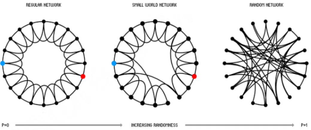
Figure 7: Watts and Strogatz models obtained by varying p between 0 and 1... 18
Figure 8: Number of new nodes introduced in the network over time. ... 30
Figure 9: Number of edges mt versus number of nodes nt in log-log scales... 31
Figure 10: Average node out-degree over time. ... 32
Figure 11: Edge density over time. ... 33
Figure 12: Degree distributions from 5 years of ucf.edu domain web graphs... 36
Figure 13: Diameter over time... 37
Figure 14: Average distance between node pairs. ... 38
Figure 15: Community discovery. ... 40
Figure 16: Community identification... 41
Figure 17: (a) edge independent paths, (b) node independent paths... 42
Figure 18: Edge betweenness of edges. ... 47
Figure 19: Edge clustering coefficient of edges. ... 50
Figure 20: Example resistor network... 54
Figure 22: Hubs and Authorities... 64
Figure 23: Degree centrality of a star, K1,8, and a cycle C8. ... 69
Figure 24: Closeness centrality of a star, K1,8, and a cycle C8. ... 70
Figure 25: An example for betweenness centrality... 71
Figure 26: An example for information centrality... 72
Figure 27: An example for clustering coefficient. ... 74
Figure 28: (a) degree centrality of the nodes in the graph, (b) corresponding edge centralities. . 77
Figure 29: Performance of community discovery using different centrality measures. ... 80
Figure 30: (a) bibliographic coupling (b) co-citation coupling. ... 81
Figure 31 : Performance on computer-generated models. ... 85
Figure 32: The Zachary Karate Club Network. ... 85
Figure 33: Communities identified in the Zachary Karate Club Network... 86
Figure 34: Communities identified in the College Football Network. ... 88
Figure 35: The largest component of the Santa Fe Institute collaboration network... 90
Figure 36: A few communities identified in the Roget's thesaurus network. ... 91
Figure 37: Communities identified in the largest component of the Santa Fe Institute collaboration network... 92
Figure 38: Output for various threshold values. ... 99
Figure 39: The architecture of UcfBot... 106
Figure 40: Implementation of the urlsToVisit data structure... 108
Figure 42: Degree distribution of a small portion of www.ucf.edu domain... 121 Figure 43: A snapshot of the network of the www.ucf.edu domain... 121 Figure 44: Overlap in communities. ... 122
LIST OF TABLES
Table 1: Size and order of the web graphs over the five-year period. t represents time. ... 29 Table 2: Comparing the complexity of the various algorithms... 67
1. INTRODUCTION
Ever since Euler’s paper on the Bridges of Königsberg [5], published in 1736, graph theory has been used to solve a wide range of problems in computer science, math, physics and chemistry. The four-color problem posed in 1852 by Francis Guthrie is considered as the birth of graph theory. This problem asks if it is possible to color, using only four colors, any map of countries such that no two neighboring countries have the same color. Appel and Haken [6] provided a solution to this problem in 1976.
Graph theory has proven itself to be a very powerful tool in solving a number of real-world problems. This is accomplished by first, modeling it as a graph and then, applying graph theoretic techniques to solve the problem. One of its first applications was on electric circuit analysis, where Gustav Kirchhoff used it to compute voltage and current in electric circuits. Many problems of practical interest can be described as graphs. Transforming a real-world problem into a graph is by itself a challenging task. For example, consider testing printed circuit boards (PCB) for short circuits. This can be accomplished by modeling the PCB into a graph such that each component on the PCB represents a vertex and an edge is drawn between two components if there is a potential for a short. Now one could perform graph coloring on this model to partition it into groups, consisting of vertices of the same color. Components represented by one group, could be simultaneously tested for shorts against all other components, thereby reducing the time required for testing. Over the past decade researchers have shown a lot of interest in graph modeling and study of properties of the graphs thus obtained.
Before proceeding further I will go over certain basic definitions, that might help the reader better understand the content of this thesis. Other definitions will be provided as and when required. For more advanced concepts and definitions in graph theory refer to [31].
A graph, G, is an ordered pair consisting of two sets (V, E), where V is a set of vertices, and E is a set of edges. The number of vertices, |V|, is termed the order of the graph and the number of edges, |E|, is termed its size. Every edge connects a pair of vertices in V, and is represented as (u, v) or eu,v. Here u, v∈ V and are called the endpoints of the edge. The graph is
termed directed if the edge (u, v) represents an ordered pair. In this case the vertex u is called the
tail and vertex v is called the head of the directed edge. Most of the graphs mentioned in this thesis are undirected unless specified otherwise. Physicists often refer to the graph as a network, vertices as nodes and edges as links. Two vertices u and v are said to be adjacent or neighbors if they are the endpoints of the same edge. The neighborhood of a vertex u, denoted Nu, is a set
consisting of all the vertices that are adjacent to u. Two edges are incident with each other if they have a common endpoint. A loop is an edge whose endpoints are equal. Two edges are said to be
parallel if they have the same set of endpoints. A vertex u is called isolated if it is not an endpoint of any edge. The degree of a vertex u, denoted du, is the number of edges that have u as
its endpoint. In a directed graph one can talk about in-degree and out-degree of a vertex. The in– degree of a vertex u refers to the number of edges that have u as its head and out-degree of a vertex u refers to the number of edges that have u as its tail. A complete graph on n vertices Kn =
(V, E), is such that V = {u1, u2,…, un} and every pair of vertices are connected by an edge i.e.E =
Graphs are being widely used to describe complex real-world systems such as the World Wide Web, Internet, energy power grids, social friendships, neural networks, etc. Despite their diversity, most of these real-world graphs share a lot of their organizational structure. Research in this area has concentrated on local (or microscopic) properties involving individual vertices or vertex pairs (e.g., shortest path between vertices, transitivity, degree distribution, robustness, etc.). Though these properties are important, it is equally important to understand their global (or macroscopic) properties. The microscopic and macroscopic properties together, aid in better understanding these systems.
1.1Real-world networks
Real-world networks are used to model complex systems, which consist of components that interact. These systems have most of the following features: agent based - the basic building blocks are characteristics and activities of individual agents in the environment under study;
dynamic – the characteristics of each of these agents vary over time, the system rarely achieves an equilibrium and the changes it undergoes are non-linear and often chaotic; organization – the agents organize themselves into groups that are well structured and these structures influence their evolution.
Network models are built to study the system and conduct scientific experiments. This involves identifying the mechanisms that characterize the dynamics of the system and translating them into sets of rules that can be implemented and investigated computationally. Care has to be taken to build simple models that provide coarse-grained description of the system. Once a
model is built researchers analytically identify new properties of the system and then validate the new properties against real-world data. Examples of complex systems and their models:
World Wide Web - The Web is an actively evolving network, composed of html pages that point to one another by means of a hyperlink. Superficially, it looks like a giant directed graph (web graph) where vertices are html pages and edges are the hyperlinks [55].
Internet – The Internet refers to the interconnected system of networks that connect computers and routers around the world. Its model consists of vertices representing computers or routers and edges representing physical connections between them [3].
Neural network – A neural network is collection of brain cells (neurons) transferring impulses to each other across via synaptic connections (axons). In this network model each vertex represents a neuron, and edges, the synaptic connections [93].
Citation network – A citation network consists of publications and their references. Vertices in this model represent publications and there exists an edge from one vertex to the other if the document being represented by the former vertex refers to the one being represented by the later [41].
Airline network – An airline network is a transportation network with vertices representing the various cities that have an airport and an edge is drawn between two vertices if there is an airline connecting the cities being represented by the vertices [48].
Semantic network – A semantic network consists of words represented by vertices and an edge between two vertices indicates that the corresponding words are either synonyms or antonyms [78].
Movie actors’ network – Nodes in this network represent actors and an edge is introduced between two vertices, if the corresponding actor’s appear in a movie together [92].
For additional examples see [3, 32, 67].
1.2Properties
Due to the randomness involved in their evolution, classical random graphs were initially used to represent real-world networks. Classical random graphs also known as Erdos and Renyi random graphs were first defined by Erdos and Renyi in the year 1959 [34]. Section 1.4.1 provides more information on these graphs. Recent studies on real-world networks have revealed some interesting structural and topological properties, which suggest that these networks are significantly different from classical random graphs. The next few sections describe a few of these properties.
1.2.1Small world network
A small world network is a network in which every vertex can reach every other vertex within a small number of hops. The idea is an extension of the small world phenomenon (small world effect) in social networks that hypothesizes that everyone in the world can be reached through a short chain of social acquaintances. Psychologist Stanley Milgram conducted an experiment and found that any two random US citizens were connected by an average of six
acquaintances [63]. Milgram sent 60 letters to various people in Omaha, Nebraska and asked them to forward them to a stockbroker in Sharon, Massachusetts. The participants were required to forward the letters to their acquaintances, whom they thought might be able to reach the stockbroker. Though Milgram’s initial experiment had a very poor completion rate, subsequent experiments by Milgram and other researchers had good completion rates. Watts and Strogatz showed the small-world phenomenon is common in a variety of realms ranging from C. elegans neurons to power grids [92]. They showed that by adding a handful of random links they could turn a disconnected network into a highly connected one. This has both positive and negative implications: a vast communication network like the internet could be made a few hops wide by addition of a few judicious routers; in contrast, in a social network, it places an individual a mere six people away from a deadly disease such as SARS. The average distance between vertices in such small world networks is of the order of log log n [27].
1.2.2Scale-free property
Barabàsi, Albert and Jeong working to study the topology of the World Wide Web [7] modeled the web as a directed graph with vertices representing HTML documents and edges representing hyperlinks or URLs that point from one document to another. They discovered that the graph thus formed had a small number of vertices with a high in/out-degree and a large number of vertices with small in /out-degree. This property was independent of the size of the graph and hence termed scale-free. This distribution of degrees was remarkably different from the Poisson distribution usually found in classical random graphs. Such a heavy tailed
degree vertices act as hubs and increase the overall connectivity of the graph thus reducing the average distance between vertex pairs. Scale-free networks are very resistant to random failure of vertices and show no sign of degradation. Due to high connectivity of hub vertices and the low probability of failure under random conditions make these networks robust. However a planned attack on the hub vertices could bring down a scale-free network in very little time. When a graph is said to exhibit the scale-free property it is also a small world [7].
1.2.3Power-law degree distribution
Figure 1: Out degree distribution of WWW.
A power-law relationship between two scalar quantities x and y can be expressed as shown below
k y ax= .
Here a is some proportionality constant and k is the exponent of the power-law. Degree distribution of a graph is a function that describes the total number of vertices in the graph with a given degree. Statistically it has been determined that for most of the real-world networks the degree distribution follows a power-law and is given by
P{du =d}= 1 dγ ,
Here P(du = d), is the probability that a vertex u has the degree d and γ is the exponent of the
power-law. Chung and Lu claim that the real-world networks have a γ value between 2 and 3 [27]. Figure 1 shows the out degree distribution of nodes in the World Wide Web, the data used was obtained from a crawl of the nd.edu domain [4].
1.2.4Network transitivity
Watts and Strogatz [92] first introduced the concept of clustering co-efficient in real world networks. It refers to the property that, two vertices, which are both neighbors of a third vertex, have a very high probability of being neighbors of one another. Section 4.1.6 provides more insight into this property. Network transitivity was introduced as an alternative to clustering co-efficient by Newman, Watts, and Strogatz [72]. The transitivity of a graph is defined as: 3 G N T N Δ Λ × = ,
where NΔ is the number of triples of vertices (v1, v2, v3) in the graph (triangles), where each
of vertices (v1, v2, v3) such that, at least one member of the triple is connected to the remaining
two. The 3 in the numerator signifies the fact that every triangle contains has three sets of triples such that, one vertex is connected to the remaining two. The resulting value of TG lies between
zero and one. The null graph has a transitivity of zero and a complete graph has the transitivity of one. Real-world networks have a transitivity value that is typically between 0.1 and 0.5 [44]. Comparatively classical random graphs have very low transitivity.
1.2.5Community structure
One property of recent interest is the community structure, it turns out the real-world networks organize themselves such that they are locally dense and globally sparse [70]. Each of these locally dense regions constitutes a community. The nodes of a community are similar in some aspect. Identifying these communities is the primary goal of my research. The community structure of a network would reflect the natural divisions of the network into densely connected subgraphs. Figure 2 shows the dominant communities present in the high school friendships network, color-coded to represent students from different races [69]. We will investigate the community structure property in detail in the following section.
1.3Community
The term community has several definitions. Initially people thought of using cliques and
near-cliques to define communities in graphs with the idea that high connectivity corresponds to similarity between vertices [9].
Figure 2: Communities in a high school friendships network.
Kleinberg while studying web graphs introduced the concept of “authorities” and “hubs”.
Authorities are web pages, which are highly referenced (vertices with high in-degree), and hubs
are web pages that reference many (high out-degree) authority pages. Later Gibson, Kleinberg and Raghavan define communities in web graph as a core of central, authoritative pages connected together by hub pages [42].
Kumar et al. define communities as bipartite cores: a bipartite core in a graph G consists of two (not necessarily disjoint) sets of vertices L and R, such that every vertex in L links to every vertex in R [57]. Vertices within L or R could be adjacent to one another.
Authority Hub
Figure 3: Hubs and authorities.
Sony Dell IBM Apple Intel ATI Hitachi Samsung Microsoft
Flake, Lawrence and Giles define them as a set of vertices C in a graph G that have more edges to members of the community than to non-members [36]. This definition of community is similar to the concept of defensive alliances introduced by Hedetniemi et al. [49]. A defensive alliance in a graph G = (V,E) is defined as a non-empty set of vertices S ⊆V such that for every vertex v∈S, |N[v] ∩S| ≥ |N[v] - S| where N[v] represents the closed neighborhood of vertex v.
v
Figure 5: Communities based on graph alliances.
within which edges are dense, but between which edges are sparse [44].
The existence of no one clear definition for community makes the task of extracting them from the graph more difficult. The general approach up until now has been to come up with a definition for the term community and then devise algorithms that would extract such structures from the input graph.
1.4Random graph models
Though the first random graph model [34] was developed in 1959, no significant developments were made till the late 90’s. Recent years have seen a high level of interest in the topology of complex networks. This has resulted in development of a number of random graph models. Most of the current work concentrates on real-world random graphs. Unlike the classical random graphs, real-world graphs are not uniformly random. They posses certain organizational-traits which are predictable. The general approach in designing these models has been as follows: a few experimentally deduced properties of real-world networks are used to design a mathematical model that exhibits these properties. The Model is then analyzed to deduce additional properties and finally the newly derived properties are validated against real-world data. This process is repeated several times to obtain models that are as accurate as possible. Having an accurate model serves several purposes: (i) it would help us understand the evolution of such networks; (ii) it would provide us with a synthetic graph to test the algorithms, developed for the real-world networks; (iii) understanding the topology of these networks would aid us in designing efficient algorithms for such networks. Despite the dynamic nature and enormous size, one of the main hurdles in working with random graphs is their non-deterministic nature.
Random graph models can be classified into two (i) static and (ii) dynamic. In a static model the vertices are added first and then edges are introduced one by one between pairs of vertices selected at random with a biased or uniform probability. In a dynamic model, at every iteration, one new vertex and a few edges are introduced that connect the new vertex to the exiting vertices (selected using a biased or uniform probability). The following sections provide some insight into the evolution of different network models and their characteristics.
⎟
1.4.1Classical random graph model
The theory of random graphs lies in the intersection between probability theory and graph theory. The Gn,m model introduced by Erdos and Renyi [34] and the Gn,p model introduced by
Gilbert [43] are known as classic random graphs. Both these models are static models. The Gn,m
model is defined as follows: Gn,m represents a set of all undirected, simple and labeled random
graphs of order n and size m. The set consists of M elements, where M =
n ⎛ ⎞ ⎜
⎝ ⎠ n× −(n 1) 2 . Each
member is a classical random graph and has a 1 |Gn m. | chance of occurring. The Gn,p model
represents a set of all undirected, simple and labeled random graphs of order n in which every potential edge of the graph occurs with a probability of p. Bollobas shows that both Gn,m and Gn,p
refer to the same graph when m= ×p M [11].
Algorithm 1 can be used to generate a classical random graph. The algorithm is very straightforward. It starts with a graph with n isolated nodes. Every edge in the graph is
n k
introduced with a probability of p. The function Rand() generates a uniform random number
between 0 and 1.
Let us now, look into some of the properties of these graphs. The degree distribution of these networks follows a binomial distribution. This can be explained as follows: Let v be a vertex picked uniformly at random from Gn,p and let P(v) denote the probability distribution
function of the random variable dv. There are (n – 1) vertices that could be adjacent to v with a
probability of p, it follows that dvwould follow a binomial distribution with the parameters (n –
1) and p, i.e., . This is in contrast to the power-law degree distributions observed in the real-world networks. The independence of the edges from one another, affects the overall transitivity of these graphs. This accounts for the low transitivity values in comparison to the real-world networks. One property that is in agreement with the real-world networks is the small-world property. It has been observed that for several values of p, G
P( )k n pk(1 p) k − ⎛ ⎞ =⎜ ⎟ − ⎝ ⎠ n,p
ClassicalRandomGraph(n, p)
V = {v1, v2, …, vn}
E’ = {e1, e2, …, enx(n-1)/2}
E = φ
forevery edge ei∈E’ do r = Rand() ifr≤pthen
E = E + {er}
endif endfor
1.4.2Watts and Strogatz model
Watts and Strogatz realized that the connection topology in real-world networks is neither completely random nor completely regular, but lies somewhere in-between [92]. They came up with a network model that could be tuned to this middle ground. They achieved this by taking a regular network (such as a ring lattice) and rewiring its edges into disarray. The end result is a highly clustered network with small average path lengths. A minimal lattice is a path, bending this linear lattice and connecting the end vertices with an edge creates a nearest-neighbor ring lattice or cycle. This consists of n vertices and n edges, and every vertex is of degree 2. If one were to include edges to the nearest-neighbors and to the next nearest-neighbors, the ring lattice would consist of 2n edges and each vertex would be of degree 4. One could create denser ring lattices by connecting the vertex to more of its nearest neighbors.
Their rewiring procedure can be explained as follows: Start with a ring lattice, which has
n vertices and k edges per vertex. For each edge e in the graph rewire one if its ends with a probability p, to another vertex, chosen uniformly at random.
Algorithm 2 can be used to create a Watts and Strogatz model random graph. The function CreateRingLattice(n, k) creates a new ring lattice graph G(V, E), where in each vertex
has k neighbors and the function GetARandomNewNeighbor(u) returns a vertex v such that v ∈ V
and initially euv ∉ E. One could tune the value of p and construct graphs that are completely random (when p = 1) or completely regular (when p = 0). For values 0 < p < 1, we get graphs with the desired properties. Figure 7 shows the graphs obtained by varying the value of p. The two properties that Watts and Strogatz were interested in particular were the average path length,
Lavg,which is a global property and clustering coefficient, Ccoeff, which is a local property. They
discovered that it is required that n >> k >> ln(n) >> 1, where k >> ln(n) guarantees that the resulting graph will be connected. It was also noted that the regular lattice at p = 0 is a highly clustered, large world where Lavg grows linearly with n, whereas the random graph at p = 1 is
poorly clustered, small world where Lavg grows logarithmically with n.
Figure 7: Watts and Strogatz models obtained by varying p between 0 and 1.
Though the Watts and Strogatz model was able to mimic the small world property found in real-world networks it failed to account for the power law degree distribution. As with the classical random graph model, the probability of finding nodes with large degree decreases exponentially.
WattsStrogratzGraph(n, k, p)
G( V, E) = CreateRingLattice(n, k) for neighbor from 1 to k do
for each c∈V do r = Rand() ifr≤pthen E = E – {ei,i + k} j = GetARandomNewNeighbor(vi) E = E + {ei,j} endif endfor endfor
1.4.3Preferential attachment model
Barabàsi and Albert proposed the preferential attachment random graph model [7]. It modeled the richer get richer behavior typically observed in social networks. Unlike the previous two models which were static this is an evolving dynamic model, defined as a discrete time process {Gt(Vt, Et)}t > 1. Let Gt(Vt, Et)refer to the state of the graph at time t. For all values
of t > 1, Gt + 1 can be obtained by applying some stochastic rules to the graph Gt. The process
starts with some m isolated vertices at time t = 0. At every incremental time step, t + 1, one new vertex, vt + 1 and m′ (m′ < m) edges are introduced into the graph. Each of the m new edges are
connected to the vertex vt + 1 at one end and at the other end they are connected to a vertex vi ∈Vt,
that is chosen at random with some bias. The probability with which a new edge would be connected to the vertex vi is directly proportional to its degree dvti.
Pt+1(vi)= dvi t dv j t j
∑
for vi ∈Vt.The main issue with this approach is that at time t = 1, P1(vi) = 0 for all vi∈V0. This is rectified
by starting with a graph, G0 that contains no isolated vertices [13]. After t time steps, the graph
has t + m nodes and m′ ×t + |E0| edges.
Algorithm 3 can be used for generating a preferential attachment model random graph. The function GenereteRandomGraph(m) generates a connected classical random graph with m
one of the vertices from the graph G with a probability proportional to its degree. The output of the algorithm would be a random graph Gt with t + m′ vertices and m′ × (t + 1) edges.
The preferential attachment model addresses several shortcomings that were present in classical random graphs: (i) it is dynamic similar to most of the real-world networks, (ii) it has the small world property, and (iii) its degree distribution follows a power law. Kumar et al. while studying frequently occurring substructures in the web graph [57], found that it contains a large number of locally dense subgraphs, and none of the models discussed so far, including the preferential attachment model contain locally dense subgraphs.
1.4.4Copy model
Kumar et al. came up with a directed dynamic random graph model [57]. They wanted to reproduce the large number of bipartite cores that occur in web graphs. To generate such a graph, one starts with a small random graph, G0 with n0 nodes at time t = 0. At each additional
time step t + 1 a new vertex, vt+1 is introduced with m′ outgoing edges. Now pick a node
(uniformly at random) from the set of already existing vertices, and call it the prototype vertex,
vpro. For every i-th outgoing edge, with a probability α, connect it to one of the existing vertices
selected uniformly at random, and with a probability 1 – α, connect it to the vertex pointed by the
i-th outgoing edge of vpro.
Algorithm 4 can be used to generate a copy model random graph. The function
GetRandomVertex(G) returns a vertex uniformly at random from the graph G and the function GetJthOutlink(v, j) returns the index of the vertex pointed by the j-th outlink of vertex v.
PreferentialAttachmentGraph(t, m′) G0(V0, E0)= GenereteRandomGraph(m′) fori from 1 to tdo Vi= Vi- 1 + {vi + m′} forj from 1 to m′ do k = GetPreferentialVertex(Gi-1) Ei = Ei – 1 + {ei m k+ ′, } endfor endfor
The intuition behind the model is as follows: each time a new web page is created it would be on a particular topic, the author of the web page would include a few hyperlinks in his page that are already present in another web page that deals in the same topic and a few new hyperlinks are added to give his web page a new flavor. The Copy model apart from being scale free and having a power law degree distribution, contains many bipartite subgraphs (bipartite cores).
1.4.5Models with embedded communities
Tawde, Oates and Glover proposed a web graph model, which has communities, embedded in them so as to satisfy the microscopic as well as macroscopic properties of the World Wide Web [88]. Unlike the previous two models, this one is not stochastic/dynamic.
They use a three-step procedure where, in the first step stand-alone communities are generated by using the preferential and random link distribution technique described by Pennock et al. in [77]. This would result in communities that have a few dangling links which would later be used to connect the community to the rest of the web. In the second step the communities generated above are combined by using the community interaction model suggested by Chakrabarthi et al. in [20]. This model is based on observed data for communities on the web. Chakrabarthi et al. experimented with 191 topics from DMoz2 and generated a 191 x 191 matrix, which modeled the interaction among these communities.
CopyModelGraph( t, m′, α) G0(V0, E0)= GenereteRandomGraph(m′) fori from 1 to tdo Vi= Vi- 1 + {vi + m′} forj from 1 to m′ do pro = GetRandomVertex(Gi - 1) r = Rand() if r < αdo k = GetRandomVertex(Gi - 1) Ei = Ei – 1 + {ei, k} else k = GetJthOutlink(vpro, j) Ei = Ei – 1 + {ei, k} endif endfor endfor
Element i, j of this matrix gives the empirical probability that an outlink, selected at random from a page in community i will link to a page in community j.The dangling links from the communities are used to perform this interconnection. Finally in the third step a benchmark link distribution of a web graph is used as a target and additional nodes and edges are added as required to achieve the link distribution of the target. Though this model is one of the very few which try to achieve an embedded community structure, it is to be noted that the model is not a purely evolving model like the ones mentioned previously.
2.
EVOLUTION OF THE WORLD WIDE WEB
2.1Importance of this work
This chapter throws some light on how the different properties of the World Wide Web evolve over time. Since its inception the World Wide Web has grown from a few thousand to several billion pages. Most of the work on real-world random networks has concentrated on their properties like degree distribution, average distance between node pairs, network transitivity, and community structure. The knowledge acquired was used to create synthetic models for these networks. Despite their dynamic nature, the above properties were studied over static instances of these networks. It would be interesting to analyze the evolution of such networks and observe how their properties change over time.
In this chapter we model the “ucf.edu” web domain as a graph and study its evolution and change in properties over a five-year period. The mapping for this model is as follows: every web page in the domain is a vertex and every hyperlink on a web page pointing to another webpage is a directed edge connecting the corresponding nodes.
There are several implications of this study: The trends and variation in properties could be used to design better models for web graphs and to evaluate existing ones. The data could be used for anomaly detection, for example, to identify spamming. Extrapolation of the collected data could help us predict properties of the network in future and also estimate its properties during a time frame when the data is not readily available. One could study the evolution of communities within these graphs and identify merging/partition of existing communities.
2.2Related work
We are aware of very few publications discussing properties of real-world networks over time. In a recent paper Leskovec et al. [61] study edge density and diameter of citation graphs, affiliation graphs, and autonomous system graphs over time. The work showed some interesting results. First, they show that the number of edges grow super-linearly in the number of nodes and claim that most of these graphs densify over time, Second, they show that the diameter shrinks over time, in contrast to priori studies which state that this parameter would grow slowly as a function of the number of nodes. Redner [81] has analyzed the properties of citation networks using the datasets obtained from the journal Physical Review. The datasets used cover citations over a 110-year period. In another independent work Katz [53] discovered densification of power laws for citation networks. Grossman [47] has performed a more statistical observation of the mathematical research collaboration graphs obtained from the journal Mathematical Reviews. Toyoda and Kitsuregawa study the evolution of communities in the “.jp” web domain [89]. They show that the distribution of size of the communities follows a power law and its exponent does not change much over time.
2.3Experimental setup
Studying graph properties at discreet time intervals has been difficult due to the lack suitable datasets. Another major draw back was storage requirements for such datasets. Web graphs are modeled based on crawls obtained by a web crawler. But these crawls can only provide us with the most recent version of the web pages. To study evolution in web graphs one needs web graph data over several years. With cost of storage decreasing, a number of
organizations have started archiving their old web pages for future reference. The Wayback Machine is an online archive that collects and stores contents of the crawls by the Alexa crawler. It has stored copies of web pages dating back to the year 1996. It provides users with a web interface to obtain archived versions of web pages when queried with an URL and date.
To construct the web graph of the ucf.edu domain we designed a special purpose downloading module on top of the UcfBot crawler, designed by myself and Cami (see Section 7), that would query the Wayback Machine archives and obtain stored versions of the web pages. Each query to the Wayback Machine consists of a URL and a date stamp. Our crawler starts with a few seed URLs that are appended with a time stamp and converted into query form. These queries are now submitted to the Wayback Machine. The page retrieved is then parsed to extract hyperlinks in the page. Each hyperlink is then converted into a query and the process is repeated until all the web pages from the specified time period are obtained.
The crawl obtained is now modeled into a web graph with each web page, representing a vertex in the graph and each hyperlink on the page pointing to another page, representing a directed edge connecting the corresponding vertices. We obtain five such web graphs by performing separate crawls one for each year from 1997 to 2001. These web graphs represent samples of the ucf.edu web domain during a particular year. The validity of our datasets depends on how comprehensive the Alexa crawls were during the past years. Our experiments show that the obtained datasets cover a large portion of the indexable ucf.edu domain during the specific time periods.
2.4Empirical observations
In this section we study the evolution of the “ucf.edu” domain by analyzing the properties of its web graphs at regularly spaced points in time. The size (number of edges) and order
(number of nodes) of our datasets are given in Table 1.
Table 1: Size and order of the web graphs over the five-year period. t represents time.
t n m 1997 7260 15998 1998 10974 16795 1999 12444 31578 2000 31170 80940 2001 58957 185909
We analyze several properties of the web graphs like number of new nodes being introduced, average degree, edge density, in-degree and out-degree distributions, diameter, and average distance between nodes. Our observations are given below.
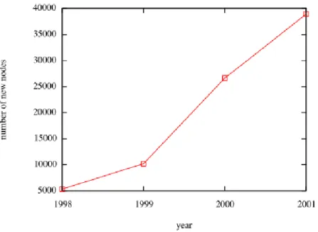
2.4.1New nodes
Using the web graph data we compute the number of nodes that were introduced into the graph every year from 1998 to 2001. This number increases steadily every year. Figure 8 shows the increase in the number new nodes over time. The x-axis represents time in years and y-axis represents the number of new nodes being introduced.
Figure 8: Number of new nodes introduced in the network over time.
2.4.2Densification power law and average out degree
Most of the existing literature about evolution of real-world networks suggests that the number of edges grows linearly with the number of nodes and as a result the average degree remains a constant. Leskovec et al. [61] observe that the number of edges grow super-linearly in the number of nodes and this growth follows a power law pattern given by:
mt∝ntγ, (1)
graph is sparse when the value of γ is close to 1 and is dense when the value of γ is close to 2. Leskovec et al. call this densification power law and suggest that networks are becoming denser over time.
Figure 9: Number of edges mt versus number of nodes nt in log-log scales.
Figure 9 shows our observations from the ucf.edu datasets. The x-axis represents the number of nodes and y-axis the number of edges in log-log scale over the five-year period. Our results echo the results from [61]. The densification exponent γ in our case has a value of 1.22. The plot in Figure 10 shows the average node out degree over the five-year period. We see that the average out degree increases over time. Though our results about super-linear growth of edges and increase in average degree coincide with the results obtained by Leskovec et al., we
see that the graphs are not getting denser over time. We explain this further in the upcoming section.
Figure 10: Average node out-degree over time.
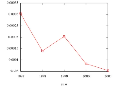
2.4.3Edge density
Edge density is the ratio of edges present in the graph to the maximum number of edges that could be present. For a directed graph the maximum number of edges is given by n ( n - 1). The change in edge density over time is shown in Figure 11, x-axis represents time and y-axis edge density.
Figure 11: Edge density over time.
Our results suggest that the edge density of these web graphs decreases over time. This seems surprising considering the fact that the average degree is actually increasing. Now we reason about this strange behavior. Edge density of a directed graph is given by
mt nt(nt −1),
where mt represents the number of edges and nt the number of nodes at time t. From equation 1
we get
mt nt(nt−1)∝
ntγ nt(nt−1),
where γ is the densification exponent. To prove that the edge density decreases over time we need to show that
ntγ nt(nt −1) ntγ+1 nt+1(nt+1−1) >1, We know that nt+1 = nt + 1. ntγ nt(nt−1) > nt +1
(
)
γ nt(nt+1), nt nt+1 ⎛ ⎝ ⎜ ⎞ ⎠ ⎟ γ > nt −1 nt+1, nt nt+1 ⎛ ⎝ ⎜ ⎞ ⎠ ⎟ γ > nt nt +1− 1 nt +1,When ntis large nt + 1 ≅nt. Substituting this in the equation proves the inequality and shows that ntγ
nt(nt−1) is a monotonically decreasing function. This explains the decreasing edge density over time.
2.4.4Degree distributions
Figure 12 shows the in-degree and out-degree distributions of our datasets during the five-year period. Each row represents a year from 1997 to 2001, the plots in the first column represent in-degree distributions and the ones in second column represent out-degree distributions. In each of the plots x-axis represents degrees and y-axis represents number of nodes. The plots for 1996 and 1997 seem to contain some noise but from 1998 the power law property is very evident. The presence of the power law, which is believed to be a basic web
In-degree distributions Out-degree distributions 1997 (a) (b) 1998 (c) (d) 1999 (e) (f)
2000
(g) (h)
2001
(i) (j)
Figure 12: Degree distributions from 5 years of ucf.edu domain web graphs.
It is interesting to note that the initial segment of the out-degree distributions deviates significantly from the power law. This has been observed by Broder et al. in [16] and they suggest that pages with low out-degree follow a different (possibly Poisson or a combination of Poisson and power law) distribution. The power-law exponents of our datasets were between 1 and 2.5, which is a bit deviant from existing datasets. We believe this is due to the small order of our graphs compared to other web graphs, which consist of at least a few hundred thousand nodes. We did observe a slowly increasing trend in the value of the power-law exponent but we see the need to further validate this observation by experimenting with datasets over a larger time period.
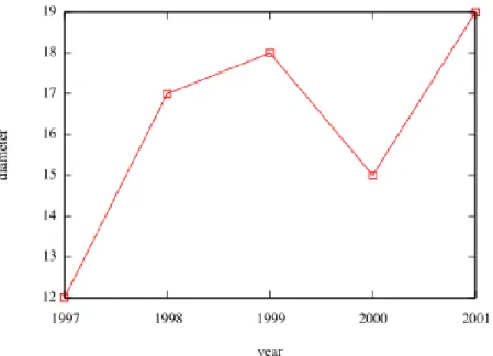
2.4.5 Diameter and average distance between node pairs
Another property of interest is the distance between nodes. There are two metrics which are often used: diameter and average distance between nodes. Diameter of a graph is defined as the longest of the shortest distances between all node pairs. We compute the diameter of the five datasets and our results are show in Figure 13, x-axis represents time and y-axis diameter. Unlike the results obtained by Leskovec et al. we did not observe any decrease in the diameter of the graphs over time. However it has to be noted that Leskovec et al. use a different definition of diameter termed the effective diameter. Effective diameter of a graph is defined as a distance d
such that at least 90% of the connected node pairs are at distance of at most d.
Figure 13: Diameter over time.
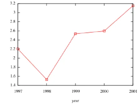
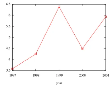
Average distance between node pairs: As stated in Section 1.2.1 this metric defines small world graphs. The average distance between nodes for the five datasets has been plotted in
Figure 14, x-axis represents time and y-axis average distance. Except for a major surge during the year 1999 the data seems to suggest that the average distance between nodes is growing at a slow rate.
Figure 14: Average distance between node pairs.
2.5Conclusion
The work proposes a new research track in the field of real-world networks. The knowledge obtained aids in better understanding the evolution of web graphs. Our results support the empirical results about super-linear growth of edges obtained by Leskovec et al. We also observe that the edge density reduces over time and explain this behavior. For future work, we would like to study, the growth and evolution of web communities; design new random graph
models that posses the observed properties; and evaluate the validity of existing random graph models.
3. SURVEY OF EXISTING METHODS
3.1Community related problemsFigure 15: Community discovery.
Two problems that are of interest are community discovery and community
identification. From a graph theoretic perspective community discovery is classifying vertices of
a graph G into subsets Ci⊆ V, 0 ≤i < k, such that vertices belonging to a subset Ci are all closely
related (classifying the nodes in a graph into different communities).
Community identification is identifying the community Ci to which a set of nodes S ⊆ V
belong (identifying the community that contains the set of vertices S). In general community
identification is considered an easier problem compared to community discovery, especially if the input graph is large.
Figure 16: Community identification.
3.2Existing algorithms
The majority of the existing community discovery algorithms employ hierarchical clustering techniques to extract communities. The hierarchical clustering algorithms work in two phases, at first, a similarity metric is defined to portray the strength of the relationship between a vertex pair. After which there are two possible ways of extracting communities using the defined metric (i) agglomerative and (ii) divisive.
The agglomerative algorithms begin by computing the similarity between every vertex pair. Initially each vertex is considered to be an individual community. During the course of the algorithm, closely related vertices are combined together to form bigger communities.
Divisive algorithms on the other hand, compute the similarity between adjacent vertex pairs. Initially the entire input graph is considered to be one large community. During the course of the algorithm, edges are removed between vertices that are least similar. This decomposes the graph into smaller but tighter communities.
Hierarchical clustering is preferred to other methods, because apart from extracting the communities it also provides their hierarchy. A general template for agglomerative and divisive algorithms is given in Algorithm 5 and Algorithm 6. S represents a matrix and its element Si,j
represents how similar vertices i and j are, all its elements are initialized to Ø; the function
Similarity(G, i, j) returns the similarity between vertices i and j; and the function Max(S) and Min(S) returns the index i, j of thelargest and smallest element in the matrix S respectively.
The final for loop could be terminated after desired number of iterations and the components that are present in G′ would represent the communities in the input graph G.
3.3Similarity metrics
The following sections provide some insight into the existing measures used to discover communities.
3.3.1Node/Edge independent paths
(a) (b) Figure 17: (a) edge independent paths, (b) node independent paths.
AgglomerativeCommunityDiscovery(G) for all vertex pairs(u, v) in G do
Su,v= Similarity(G , u, v) endfor V′ = {v1, v2, …, vn} E′ = {∅} for i from 1 to n(n−1) 2 do u,v = Max(S) E′ = E′ + {eu,v} Su, v = 0 endfor
Algorithm 5: Template for agglomerative procedure.
DivisiveCommunityDiscovery(G) for alleu,v∈E do
Su,v= Similarity(G, u, v) endfor V′ = V E′ = E for i from 1 to |E| do u,v = Min(S) E′ = E′ - {eu,v} Su, v = NULL endfor
To the best of my knowledge there are no prior publications utilizing node/edge independent paths as a similarity metric. Girvan and Newman first suggested this concept in [44]. Two or more paths are vertex-independent (vertex-disjoint) if they don’t share any vertex except maybe the initial and final vertices. Similarly, two or more paths are edge-independent (edgedisjoint) if they don’t share any edges. Existence of a large number of vertex (edge) -independent paths between a vertex pair indicates better similarity.
The intuition behind this approach is that the number of vertex (edge)-independent paths between vertices in the same community is greater than the number of vertex (edge)-independent paths between vertices in different communities. It is know that the number of vertex (edge)-independent paths between a vertex pair i, j is equal to the minimum number of vertices (edges) that need to be deleted to disconnect i and j [62].
The number of edge independent paths can be obtained by using the max-flow algorithms. Each edge is assumed to posses a unit flow capacity. The cardinality of the min cut would give the number of edge disjoint paths. Algorithm 7 describes the procedure to obtain edge independent paths between a given pair of vertices.
EdgeIndependentPathSimilarityMetric(G, i, j) s = i t = j G′(V′, E′) = G(V, E) for alleuv∈E′do Cuv = 1 endfor M = MinCut(G′, C, s, t)
The algorithm first assigns one of the input vertices as a source and the other as a sink. Then each edge is assigned a unit flow capacity. The function MinCut(G, C, s, t) computes the
min cut of the graph G with edge capacities specified by matrix C where s is the source and t is the sink. M would contain the set of edges that form the min cut and |M| is the number of edge independent paths between i and j. If one were to use the Edmonds-Karp algorithm to compute the min cut then the complexity of the above approach would be O(nm2). For a sparse graph m≈
n and the complexity is O(n3). Since this has to be computed for all vertex pairs, the overall complexity is O(n5).
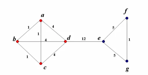
3.3.2Edge betweenness
Girvan and Newman [44] proposed the idea of edge betweenness as a similarity measure based on the concept of vertex betweenness introduced by Freeman [39]. Vertex betweenness of a vertex is defined as the number of shortest paths between pairs of vertices that pass through the given vertex. Edge betweenness of an edge is defined as the number of shortest paths between pairs of vertices that pass through the given edge. Betweenness in general is a centrality measure used to portray the importance of a vertex/edge within a graph. Centrality is discussed in detail in Section 4.1. This measure is only suited for divisive algorithms, as the value of edge betweenness for node pairs that are not adjacent is not defined.
Figure 18: Edge betweenness of edges.
The edge betweenness of inter-community edges would be high, as the shortest paths between nodes in the two different communities would have to pass through them. After computing the edge betweenness of all the edges, one can remove the edges with high edge betweenness and expose the community structure. Figure 18 describes a graph where the weights of the edges represent their betweenness. Clearly the inter-community edge ede has a higher value
of betweenness than all the other edges.
The divisive algorithm proceeds as follows: first the edge betweenness of all the edges is computed, the edges with the highest value for edge betweenness is deleted and the edge betweenness of the remaining edges is re-computed. The whole process is repeated for desired number of iterations or until all the edges are removed. Re-computing the edge betweenness, after every iteration is necessary, without which the results were not very impressive.
Computing the shortest path between a vertex pair takes O(m) time. Since we need to compute the shortest path between n2 vertex pairs, one might assume it would take O(mn2) time
to compute the betweenness of all the edges. In fact computing the shortest path from one vertex to the remaining n – 1 takes O(m) time. In effect computing all the shortest paths can be accomplished in O(mn) time. The algorithm requires the betweenness to be computed after removal of an edge. Hence the overall complexity of the algorithm is O(m2n). For a sparse graph
m≈n and the complexity is O(n3).
Algorithm 8 can be used to compute the edge betweenness of all the edges in the graph. At first the shortest paths from vertex s to all other vertices is calculated. Then the number of shortest paths are computed by traversing the graph from a leaf node to the source. During the traversal we count the number of successor edges to each edge. This counts the number of shortest paths through an edge. Repeating these steps from every vertex s in the graph and then consolidating the sum of the counts provides us with required betweenness.
One of the main drawbacks of the divisive algorithms is that they fail in scenarios where the edges do not portray the community structure. For example a bipartite graph consists of two sets of vertices, and no edges exist between vertices in the same set. Each of these sets would constitute a community. Removal of edges in any order using a divisive algorithm would not reveal the two communities. The cubic complexity of the algorithm makes it impractical for graphs with a few thousand nodes.
EdgeBetweennessSimilarityMetric(G) for s from 1 to ndo
s = 1
Ds = 0 Ws = 1
for all i such that eis∈E do Di = Ds + 1
Ws = 1 Wi = 1
endfor do
for all j such that eij∈E do
ifDj == NULL then Dj = Di + 1 Wj = Wi
else if Dj≠ NULL and Dj = Di + 1 then Wj = Wj+ Wi
else if Dj≠ NULL and Dj < Di + 1 then
endif endfor
while we have no vertex i such that eij∈E and Di≠ NULL and Dj== NULL
for every leaf node t do
for all i such that eit∈E do BBit = BitB + Wi Wt
endfor endfor
foreij∈E from the farthest eij to closest eij to node sdo
for ejk∈E where ejk farther than eij to node sdo BBij = BijB + (BBjk + 1) * Wi Wj
endfor endfor
endfor
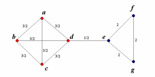
3.3.3Edge clustering co-efficient
Figure 19: Edge clustering coefficient of edges.
Radicchi et al. came up with an algorithm that utilizes the local property of the graph rather than a global property like the edge betweenness or node/edge independent paths. They devised a new similarity measure called the edge clustering co-efficient [79]. The Edge clustering co-efficient of an edge is defined as:
, 1 , min( 1, 1) i j i j T d d + − −
where Ti,j represents the number of triangles, K3’s, to which the edge i, j belongs to and di
represents the degree of node i. The denominator min(di - 1, dj - 1) indicates the maximum
number of triangles to which the edge eij could belong. The “+ 1” in the numerator takes care of
Algorithm 9 can be used to compute the edge clustering co-efficient of an edge (i, j). Once the clustering coefficient of all the edges is computed, the edge with the lowest value of clustering coefficient is removed. As in the edge betweenness algorithm, Radicchi et al. suggest re-computing the clustering coefficient of the set of edges that might be affected by removal of the edge. Deleting edges with low edge clustering coefficient value removes the inter-community edges and exposes the underlying communities. The complexity for computing the clustering coefficient for all the edges takes > O(m2) time. Clearly the algorithm would fail on all triangle free graphs.
The motivation behind this algorithm is as follows: the density of edges is higher inside the communities than along its boundaries. As a result edges connecting nodes in different communities are included in few or no triangles, on the other hand edges connecting nodes in the same community would be a part of many triangles and consequently have a high clustering co-efficient value. One could repeat the above algorithm by counting the number cycles of length four (squar