Methods for Learning Directed and Undirected Graphical Models

(1)

Department of Computer Science Series of Publications A

Report A-2020-1

Methods for Learning Directed and Undirected

Graphical Models

Janne Lepp¨

a-aho

Doctoral dissertation, to be presented for public examination with the permission of the Faculty of Science of the University of Helsinki, in Auditorium B123, Exactum, on January 24th, 2020 at 12 o’clock noon.

University of Helsinki Finland

(2)

Supervisor

Teemu Roos, University of Helsinki, Finland Pre-examiners

Joe Suzuki, Osaka University, Japan

Wray Buntine, Monash University, Australia Opponent

Brandon Malone, NEC Laboratories Europe, Germany Custos

Teemu Roos, University of Helsinki, Finland

Contact information

Department of Computer Science P.O. Box 68 (Pietari Kalmin katu 5) FI-00014 University of Helsinki Finland

Email address: [email protected] URL: http://cs.helsinki.fi/ Telephone: +358 2941 911

Copyright c2020 Janne Lepp¨a-aho ISSN 1238-8645

ISBN 978-951-51-5771-3 (paperback) ISBN 978-951-51-5772-0 (PDF) Helsinki 2020

(3)

Methods for Learning Directed and Undirected Graphical Models

Janne Lepp¨a-aho

Department of Computer Science

P.O. Box 68, FI-00014 University of Helsinki, Finland [email protected]

PhD Thesis, Series of Publications A, Report A-2020-1 Helsinki, January 2020, 50+84 pages

ISSN 1238-8645

ISBN 978-951-51-5771-3 (paperback) ISBN 978-951-51-5772-0 (PDF) Abstract

Probabilistic graphical models provide a general framework for modeling relationships between multiple random variables. The main tool in this framework is a mathematical object called graph which visualizes the as-sertions of conditional independence between the variables. This thesis investigates methods for learning these graphs from observational data. Regarding undirected graphical models, we propose a new scoring criterion for learning a dependence structure of a Gaussian graphical model. The scoring criterion is derived as an approximation to often intractable Bayesian marginal likelihood. We prove that the scoring criterion is consistent and demonstrate its applicability to high-dimensional problems when combined with an efficient search algorithm.

Secondly, we present a non-parametric method for learning undirected graphs from continuous data. The method combines a conditional mu-tual information estimator with a permutation test in order to perform conditional independence testing without assuming any specific paramet-ric distributions for the involved random variables. Accompanying this test with a constraint-based structure learning algorithm creates a method which performs well in numerical experiments when the data generating mechanisms involve non-linearities.

For directed graphical models, we propose a new scoring criterion for learning

(4)

iv

Bayesian network structures from discrete data. The criterion approximates a hard-to-compute quantity called the normalized maximum likelihood. We study the theoretical properties of the score and compare it experimentally to popular alternatives. Experiments show that the proposed criterion provides a robust and safe choice for structure learning and prediction over a wide variety of different settings.

Finally, as an application of directed graphical models, we derive a closed form expression for Bayesian network Fisher kernel. This provides us with a similarity measure over discrete data vectors, capable of taking into account the dependence structure between the components. We illustrate the similarity measured by this kernel with an example where we use it to seek sets of observations that are important and representative of the underlying Bayesian network model.

Computing Reviews (2012) Categories and Subject Descriptors:

Computing methodologies→ Machine learning

Mathematics of computing→ Probability and statistics Mathematics of computing→ Bayesian networks Mathematics of computing→ Markov networks General Terms:

machine learning, probabilistic graphical models, model selection Additional Key Words and Phrases:

Bayesian networks, Markov networks, Bayesian statistics, information theory, pseudo-likelihood, mutual information, normalized maximum likelihood, Fisher kernel

(5)

Acknowledgements

I would like to thank my supervisor Professor Teemu Roos for all the guidance and support during my PhD studies. I really appreciate the free and inspiring working environment that has been present throughout my PhD journey.

I am grateful to pre-examiners, Professors Joe Suzuki and Wray Buntine, for taking time to go through this manuscript carefully and providing comments at short notice. I would also like to thank Dr Brandon Malone for agreeing to be the opponent in my defence.

A big thanks goes to all the co-authors of the joint publications included in this thesis. I would especially like to thank Dr Tomi Silander for sharing great ideas and collaboration that resulted in two publications.

I would like to thank all the members, past and present, of the ”Informa-tion, Complexity and Learning” research group: Jussi Määttä, Yuan Zou, Ville Hyvönen, Elias Jääsaari, Teemu Pitkänen, Jukka Kohonen, Ioanna Bouri, Santeri Räisänen, Sotiris Tasoulis, Yang Zhao and Quan (Eric) Nguyen.

I acknowledge the financial support from Doctoral Programme in Com-puter Science (DoCS) and Academy of Finland (COIN CoE and project TENSORML).

Finally, my heartfelt thanks go to all my friends and family. My parents, Jaakko and Eija-Liisa, thank you for always being there and providing support and encouragement.

And Aurora, your unconditional love and support has been the biggest thing that kept me going through this journey.

Helsinki, December 2019 Janne Lepp¨a-aho

(6)

(7)

Original publications

This thesis is based on the following publications. They are reprinted at the end of the thesis.

I. J. Lepp¨a-aho, J. Pensar, T. Roos, and J. Corander. Learning Gaussian graphical models with fractional marginal pseudo-likelihood.

Interna-tional Journal of Approximate Reasoning, 83:21 – 42, 2017.

II. J. Leppä-aho, S. Räisänen, X. Yang, and T. Roos. Learning non-parametric Markov networks with mutual information. In V. Kra-tochv´ıl and M. Studený, editors,Proceedings of the Ninth International

Conference on Probabilistic Graphical Models, volume 72 of

Proceed-ings of Machine Learning Research, pages 213–224, Prague, Czech

Republic, 11–14 Sep 2018. PMLR.

III. T. Silander, J. Leppä-aho, E. Jääsaari, and T. Roos. Quotient nor-malized maximum likelihood criterion for learning Bayesian network structures. In A. Storkey and F. Perez-Cruz, editors, Proceedings of the Twenty-First International Conference on Artificial Intelligence

and Statistics, volume 84 ofProceedings of Machine Learning Research,

pages 948–957, Playa Blanca, Lanzarote, Canary Islands, 09–11 Apr 2018. PMLR.

IV. J. Lepp¨a-aho, T. Silander, and T. Roos. Bayesian network Fisher kernel for categorical feature spaces. Accepted for publication in

Behaviormetrika, 2019.

Author contributions:

Article I: JL formulated and proved the consistency results, performed the experiments and wrote the majority of the paper.

Article II: Based on the idea and preliminary work by SR, XY and TR, JL implemented the method, performed the experiments, and wrote the paper.

(10)

x Contents

Article III: JL proved the consistency and the regularity of the method, wrote the corresponding sections, and took part in analyzing the experimen-tal results.

Article IV: JL proved the invariance theorem, implemented the method, performed the experiments and participated in writing the paper.

(11)

Chapter 1 Introduction

I don’t know what that would be — I like graphs. And that doesn’t mean I’m going to try to build one. I’m looking for something more like the following graphs. An excerpt from the output of

GPT-2 language model built by Adam King when inputted: ”This is a nice quote for a computer science PhD thesis:”.

This chapter provides a gentle introduction to probabilistic graphical models. Graphical models have been around already for couple of decades and there exists several thorough overviews regarding the subject [25, 29, 63]. We scratch the surface here, going through the general framework briefly and then turn our focus to the main question addressed in this thesis, the problem of learning the structures of graphical models from a set of data. We conclude the chapter by describing the outline for the rest of the chapters and summarize the contributions of the original articles forming this thesis.

1.1 Probabilistic graphical models

Probabilistic graphical models provide a convenient tool for representing and analyzing complex probability distributions over multiple random variables. The graphical models considered in this thesis consist of two main building blocks: 1) a collection of random variables whose joint distribution we are interested in modeling; and 2) a graph, a mathematical object that contains

(12)

2 1 Introduction

one node for each random variable and a set of edges between these nodes. The edges in the graph can be undirected or directed, depending whether we are considering Markov networks (equivalently undirected graphs) or Bayesian networks (directed acyclic graphical models). Regardless of which of these two model classes we are using, the graph depicts relationships between the variables by encoding certain assertions of conditional inde-pendence that are present in the joint distribution. As such, the graph provides a visual representation of the dependence structure, making some properties of the complex multivariate distribution readily available at a glance, and what is more, the graph can be often used to decompose the distribution into smaller components that admit easier interpretation and are more tractable to handle computationally.

By providing a very general framework for representing multivariate distributions, graphical models are applied widely in the fields of machine learning and statistics. For instance, the structures of many commonly encountered models in these areas are easily described using a directed graphical model. Some classical examples include [4]: mixture models, (probabilistic) principal component analysis, factor analysis, naive Bayes,

and also, to name a more recent example, variational auto-encoders [24]. When treating graphical models, the discussion separates intrinsically in three distinct topics [25]: representation,inference, andlearning. We started our discussion by noting how graphical models are a tool for representing complex probability distributions. Then, having specified the distribution with the help of a graph, we might want to use our model to answer probabilistic queries regarding some of the variables. This is the part where the inference comes into play and often the graph structure is in the key role by determining how efficiently we can run our inference procedures. However, the part we are dedicating most of the focus in this thesis is the learning which tackles the problem of coming up with the graphical model in the first place.

1.2 Learning graphical models

In the learning part, we are given a set of observed data on some variables and our goal is to learn the graph that specifies the dependence structure among variables. This part is called structure learning. Additionally, we might also be interested in learning the parameters for this structure which might involve a separate step or happen at the same time with the structure learning, depending on the used method.

(13)

1.3 Outline of the thesis 3 The motivation for structure learning might be knowledge discovery: by learning the graph, we gain insight on the variables in our domain as we know how they depend on each other. For instance, directed graphical models have been used to model potential relationships in protein signaling networks [47] and brain-region connectivity using fMRI data [19]. The graph learning might also be motivated as an initial step for the subsequent prediction or inference tasks. For instance, in a classification task, we are interested in predicting the value for a class variable given the values for predictor variables. Examples of graphical models that are learned with the classification in mind include: naive Bayes, tree augmented naive Bayes [13] and limited dependence Bayesian network [48] classifiers.

In general, the learning of graphical models is a challenging problem. For the undirected graphs, the number of possible graphs increases exponentially with respect to the number of variables. In case of directed acyclic graphs, there exists even more possible graph structures for a given set of variables. The approaches for learning graphical models are commonly divided in two categories. The score-based methods cast the learning as a model selection problem. In this approach, each graph implies a model over our data that we can score using some criterion. The learning reduces thus to finding the highest scoring structure.

The constraint-based methods approach the problem from a different

angle. They utilize the fact that the edges in the graphical model imply a set of conditional independence statements over the variables. Based on the observed data, we can test whether a particular independence statements are likely to hold with the help of the well-known machinery from statistical literature calledhypothesis testing.

1.3 Outline of the thesis

This thesis studies the learning of graphical models in different scenarios. Without yet going much into the details, we will be tackling the following kinds of questions:

• Assume that we have a large number of variables and possibly a small amount of observations. Assume further that we model the data with a multivariate normal distribution. How can we learn an undirected graph describing the dependence structure of variables?

• What about if we do not want to make restrictive assumption of multivariate normality? Here, we focus on situations where the number of variables is relatively small but the variables might depend on each

(14)

4 1 Introduction

other in a complex, non-linear way. How do we learn an undirected graph in this situation?

• Assume now that the variables are categorical and we want to learn a directed acyclic graph. Adopting a score-based approach, there are plenty of scoring functions to choose from, each with its own virtues and vices. Can we come up with a new one that would avoid at least some of the shortcomings of the previous approaches?

In addition to problems related to learning, we also consider one appli-cation where we make use of the learned Bayesian network. We start with a completely specified Bayesian network model over categorical variables. Using this network we address the following problem:

• How can we measure similarity among data vectors with the aid of our Bayesian network? In general, being able to compute similarity for categorical data would give rise to myriad of applications but what would be the thing that this model induced similarity is the most suitable for?

The rest of the thesis is organized as follows. After providing the summaries of the original articles in this thesis, we move on to the Chapter 2 where we dive into the world of graphical models in an increased level of formality, providing notations and concepts needed to grasp the content of the remaining chapters. Then the two subsequent chapters treat the content of the original articles: Chapter 3 is based on original articles I and II with an underlying theme of learning undirected graphical models, and articles III and IV are discussed in Chapter 4, where the main topic is directed acyclic graphs. Chapter 4 is not purely focused on learning as we also present an application on how to make use of the learned networks. Finally, conclusions are presented in Chapter 5.

1.4 Main contributions

In this section, we briefly summarize the main contributions of the original articles.

Article I: Learning Gaussian graphical models with fractional marginal pseudo-likelihood. We propose a new scoring criterion for learning the dependence structure of the Gaussian graphical model. The criterion makes use of pseudo-likelihood in order to express the approxi-mative marginal likelihood for any undirected graph in closed form. It is

(15)

1.4 Main contributions 5 applicable in high dimensional settings and also shown to be consistent. In the experiments, we pair the criterion with an efficient greedy algorithm and evaluate the performance of the method against the leading methods for learning Gaussian graphical models.

Article II: Learning non-parametric Markov networks with mu-tual information. We propose a method for learning Markov network structures without restricting the learned network to belong to any spe-cific family of parametric distributions. The method makes use of a non-parametric estimator of conditional mutual information to test independence assertions. The resulting independence test is combined with a constraint-based learning algorithm, and shown to work well in the settings where the relationships between variables involve non-linearities.

Article III: Quotient normalized maximum likelihood criterion for learning Bayesian network structures. We present a new scoring criterion for learning Bayesian network structures in the discrete setting. The criterion is motivated as an approximation to information theoretic quantity called Normalized Maximum Likelihood. We discuss the theoretical properties of the score and compare it empirically to other commonly used criteria.

Article IV: Bayesian network Fisher kernel for categorical feature spaces. In this article, we derive a closed form expression for a Fisher kernel derived from a general Bayesian network model over categorical variables. We show that the resulting kernel is invariant for Bayesian networks expressing the same assertions of conditional independence. The Bayesian network Fisher kernel is studied empirically in experiments where the aim is to use the kernel to gain insight into the underlying Bayesian network.

(16)

(17)

Chapter 2 Preliminaries: graphical models

This chapter introduces the notation and basic concepts related to graphical models. After the overview, we start with the Bayesian networks and then move on to the undirected graphical models. With the general notation fixed, we then discuss the structure learning of graphical models more in detail.

2.1 General notation

Let X = (X1, . . . , Xd)T denote a d-dimensional random vector. Let G= (V, E) denote a graph, whereV ={1, . . . , d} is the set of nodes and E ⊂

V ×V denotes the set of edges. We associate each random variable Xi with the node i∈V, i= 1, . . . , d. The terms node and variable are used interchangeably. We useXA, A⊂ {1, . . . , d} to refer to a subvector of X restricted to variables in the setA.

The edges in the graph can be directed or undirected. In this thesis, we treat only graphs that include one of the aforementioned type at a given time. We say that there exists a directed edge fromXi to Xj, denoted also asXi →Xj, if and only if (i, j)∈E. If (i, j)∈E, variableXi is said to be a parent ofXj. In case of an undirected edge between Xi and Xj, Xi−Xj, the edge set E contains tuples (i, j) and (j, i).

2.2 Directed graphical models

This section considers Bayesian networks, or equivalently, directed acyclic graph (DAG) models. Assume thatGis a directed acyclic graph, implying that all the edges are directed and there does not exist any directed cycle in

G. Let p(X) denote the joint distribution of X. The graphGencodes a set 7

(18)

8 2 Preliminaries: graphical models

of conditional independence assertions between the components ofX that can be characterized withMarkov properties[29]. The local directed Markov

property states that each variable Xi is independent of itsnon-descendants

given its parentsXπ(i). A variable Xi is non-descendant ofXj if there does not exist a directed path from Xj to Xi. We use π(i) = {j | (j, i) ∈ E} to denote the parent set of variable Xi. The local Markov property is equivalent to the following factorization ofp(X) according toG:

p(X) = d

Y

i=1

p(Xi |Xπ(i)). (2.1)

This decomposition (2.1) to a product of conditional distributions is sometimes referred as the chain rule for Bayesian networks. It allows us to parametrize the joint distribution p(X |θ) conveniently through defining local parametersθi for each conditional distribution p(Xi |Xπ(i), θi).

For instance, assuming our variables are continuous, we can take condi-tional distributions to be linear Gaussian

Xi |Xπ(i)=xπ(i) ∼ N(wTi xπ(i), σ2i), (2.2) with the local parameters θi being now the vector of edge strengths wi which defines the mean of the distribution and the conditional variance σ_i2. If we define the conditional distributions using (2.2), the joint overX will be a multivariate normal N_d(0,Σ), where Σ can be determined from the collection of the local parameter sets [38].

Assume next that the variables are discrete, meaning that each Xi can take values from 1 to ri ∈N\ {0,1} (variables are treated categorical even though encoded using integers). In this case, it is common to parametrize the DAG structure using conditional probability tables by enumerating all the possible combinations of values for parentsXπ(i) of Xi, and defining

θijk=P(Xi =k|Xπ(i)=j), (2.3) where i ∈ {1, . . . , d}, k ∈ {1, . . . , ri} and j ∈ {1, . . . , qi} with qi denoting the number of possible parent combinations andXπ(i)=j meaning that the parent variables take values according to the jth configuration. For each i, the local distribution containsqi·(ri−1) free parameters, as the probabilities need to sum to one for any given parent combination. In other words, we model each variable with one categorical/multinomial distribution for each possible assignment of its parent variables. The parameter vectors related to these conditional distributions are denoted by θij ={θijk|k= 1, . . . , ri}.

(19)

2.3 Undirected graphical models 9 This allows us to express the likelihood of θfor a single data pointX=x as

p(x|θ, G) = d Y i=1 qi Y j=1 ri Y k=1 θ_ijkI(xi=k, xπ(i)=j), (2.4)

where the indicator functionI(xi =k, xπ(i) =j) = 1 ifxi =kandxπ(i)=j; andI(xi =k, xπ(i) =j) = 0, otherwise.

With directed graphical models it is possible that two different DAG structuresG1 andG2 represent exactly the same assertions of conditional independence. The graphsG1 andG2 are then said to independence equiva-lent. In case of the above two examples where the conditional distributions are linear Gaussian or multinomial, independence equivalence implies also that the two DAGsG1 and G2 represent the same set of joint distributions overX [14].

2.3 Undirected graphical models

The undirected graphical models (Markov networks), as the name implies, represent the independence structure for a set of random variables with the help of an undirected graphG. The possible sets of conditional inde-pendence assertions that can be represented with undirected graphs are generally different from those we can represent using DAGs. However, there exists a class of graphs calledchordal or decomposable graphs consisting of independence structures that are equally well representable using DAGs or undirected graphs.

Also in the undirected case, we can characterize the independence assumptions using similar Markov properties as those mentioned in the directed case. Since the edges do not have directions, we do not have concepts like ”parent” or ”child” and the properties admit maybe a bit simpler form.

Let mb(i) denote the Markov blanket of variable Xi. The set mb(i) includes all nodes that are connected to i by an edge in G. Now, the

pairwise, local, and global Markov properties can be stated as follows:

1. If there is no edge betweenXi andXj, the variableXi is independent of Xj given the remaining variables.

2. Given its Markov blanket, each variableXi is conditionally indepen-dent of all the remaining variables.

3. For disjoint subsets of nodes,A, B, C⊂V, it holds thatXA is condi-tionally independent of XB givenXC, if C separatesA and B in the graph G.

(20)

These three properties are equivalent assuming the positivity of the distri-bution p(X) [29].

Even though the independence assertions are somewhat easier to look up from an undirected graph, the distribution does not in general factorize into as intuitive components as the conditional probability distributions in case of DAGs. With Markov networks, the distribution factorizes over the

maximal cliques of the graph. A clique is a set of nodes in a graph such

that each node is connected by an edge to all the remaining nodes in the clique. Moreover, a clique is maximal if there does not exist a node in the graph which could be added to it while still satisfying the clique definition. LetC denote the set of maximal cliques inG. Now,

p(X) = 1

Z

Y

C∈C

φ(XC), (2.5)

where φ(XC) are called clique potentials which map the values of ran-dom variables to (usually) strictly positive values. The term Z−1 =

P

x

Q

C∈Cφ(XC = xC) is the normalization constant which guarantees that the product defines a valid distribution. In case of continuous variables the sum would be replaced by an integral. As the requirement for a mapping to be a potential function is rather loose, we generally lose the ability to interpret these as probability distributions.

One specific class of undirected graphical models encountered also later in this thesis is Gaussian graphical models. In Gaussian graphical models, we have an undirected graph Gand a random vector X following a multi-variate normal distributionN_d(0,Ω−1), where the matrix Ω is the inverse of covariance, aka the precision matrix. Due to the properties of multivariate normal distribution, the graph structure is easily read from the precision matrix. To be more precise, Xi is conditionally independent of Xj given the rest of variables if, and only if Ωij = 0. This means that there is no edge between these variables in the graph G. In other words, in undirected Gaussian graphical models, the graph structure is visible in the zero pattern of Ω but otherwise the elements are unrestricted as long as the resulting matrix is positive definite.

2.4 Graphical model structure learning

In this section, we define the problem of learning the structure of graphical model a bit more carefully, review the outlines of the common strategies when tackling this problem and mention some related concepts we will encounter later in the thesis.

(21)

2.4 Graphical model structure learning 11 2.4.1 Defining the problem

In every article included in this thesis, we are either proposing a method for solving, or just encountering the following problem: we are given a data matrixX = (x1, . . . ,xn) consisting ofd-dimensional observations xj. Depending on the problem, componentsxj_i might be real numbers or integers representing the values of continuous or categorical variables, respectively. We have the underlying assumptions thatxj are realizations of independent and identically distributed (i.i.d.) random variables following a distribution whose dependence structure obeys the Markov properties implied by graph

G. Based on the observational data X, our aim is to recoverG.

Next, we will discuss the score-based methods and how they approach this problem.

2.4.2 Score-based learning

The score-based approach treats the problem of learning a graph structure as a model selection problem. With dvariables, we have a finite amount of possible graphsG to choose from, and each graph is associated with a modelMG for our data. Model

MG={ p( · |G, θ)|θ∈ΘG⊆Rk }

means here a set of probability distributions for dataX that have a common functional form depending onG, and that are indexed by somek-dimensional parameter vectorθ.

A scoring function is mapping which returns a scalar value for every admissible input ofX andG. We can interpret this scalar value to describe how well our model fits the observed data. Making our models more complex, we can naturally fit the data better, thus scoring functions usually include a term that takes into account the complexity of the model, making the total score a trade-off between the goodness-of-fit and model complexity penalty.

There exists a wide variety of possible scoring functions devised under different assumptions. In this thesis, we will discuss scoring functions that draw their motivation from Bayesian statistics [2, 15] and Minimum Description Length (MDL) principle [17, 44].

With the scoring function given, the learning problem becomes an optimization problem over the possible graph structures. When learning DAGs, most of the scoring functions aredecomposable, meaning that the score for the whole network can be expressed as a variable-wise product (or a sum) where the ith local term depends only on the data on Xi and its parents Xπ(i). This allows the score to be optimized by traversing the

(22)

space of graphs with the help of local updates that affect only a couple of terms in the decomposition. Decomposability is not that often encountered when learning undirected graphs, although we will see a counter-example in Chapter 3.

Another theoretical property that we will discuss later in the thesis when proposing new scoring functions is consistency. Consistency roughly guarantees that our scoring function will eventually give the highest score to the true generating graph as we let our data sizen tend to infinity. 2.4.3 Constraint-based learning

In the constraint-based approach, we make use of the fact that the graph defines a certain set of independence assumptions over the variables in our domain. These are the Markov properties we reviewed earlier. Based on the observed data, we can then perform a series of queries to try to find Markov properties that hold and parse our graph together from these results. In practice, a single query is a conditional independence test which can be formulated as a hypothesis test. For an overview on hypothesis testing, see Casella and Berger [6].

The result of performing a hypothesis test is a yes/no answer, which usually indicates a presence or absence of an edge in the graphical model. Various algorithms have been proposed in order to be able to learn the network structures efficiently without resorting to testing every possible assertion of conditional independence.

For instance, in Chapter 3, we will use an algorithm that makes use of the local Markov property when learning an undirected graph. The idea is to find the Markov blanket for each variable, eq. the smallest set of variables that renders the variable conditionally independent of the remaining ones.

(23)

Chapter 3 Learning undirected graphical

models

In this chapter, we discuss two methods for learning undirected graphical models with continuous variables that differ greatly in modeling assumptions they are making about the underlying data generating distribution. In the first approach, we model our data with a multivariate normal distribution, and using an approximation to the likelihood called pseudo-likelihood, we derive a computationally attractive scoring function, titled as fractional marginal pseudo-likelihood (FMPL), that allows us to learn graphs with very large number of variables. In the second part, we devise a test for conditional independence that does not require us to assume any particular parametric form of the distribution for the variables involved. This allows us to identify complex interactions among variables more accurately but the resulting method is also computationally more involved.

3.1 Learning high dimensional Gaussian

graphi-cal models

We assume that our dataX = (x1, . . . ,xn) are i.i.d samples from a multi-variate normal distribution N_d(0,Ω−1), where the structure of the (positive definite) precision matrix Ω is determined by some undirected graph G∗, which describes the dependency structure of the generating distribution. In other words, we are modeling our data using the Gaussian graphical model (GGM), mentioned in Chapter 2.

(24)

14 3 Learning undirected graphical models

3.1.1 Bayesian learning of GGMs

We adopt a score-based approach to learning and make use of the Bayesian framework in deriving our scoring function. To briefly summarize, the Bayesian approach requires us to first construct a joint probability model for all the relevant quantities (observed and unobserved) in our problem domain, which involves expressing our beliefs on unobserved quantities by assigning prior distributions over them. Next task is to compute the posterior distribution for quantities under interest, and then finally use this posterior as the basis of decision making. In the context of score-based learning, Bayesian approach boils down to finding the graph with the highest posterior probabilityp(G|X). The posterior for Gcan be written as follows:

p(G|X)∝p(X, G) =p(X |G)·p(G), (3.1) wherep(G) is the prior probability forGandp(X |G) denotes the marginal likelihood. In the first proportionality, we omitted the term p(X) as this is constant for everyG, and can be ignored when we are only interested in finding theG with the maximum posterior probability. Marginal likelihood is the only data dependent term in Eq. (3.1). It is defined as follows:

p(X |G) =

Z

θ∈ΘG

p(X |θ, G) p(θ|G) dθ, (3.2)

where ΘG denotes the set of possible parameter values under G. Assuming uniform prior over graphs, the structure learning problem reduces to finding the graph with the highest marginal likelihood. However, even with our Gaussian assumption, there are several problems when trying to evaluate the marginal likelihood integral under a general graph structureG:

1. We need to be able to specify the parameter prior p(θ |G) for any given network structure. Eliciting the prior distributions subjectively might quickly become a daunting task as the number of variables increases.

2. Marginal likelihood is easily1 evaluated in closed form only if the underlying graph is chordal [10].

3. Methods based on numerical approximations of marginal likelihood tend to get computationally very demanding as the number of variables grows. For instance, Wang and Li [62] report that approximating the

1_{Recent work [60] shows that there exists, in principle, a way to evaluate marginal}

(25)

3.1 Learning high dimensional Gaussian graphical models 15 marginal likelihood of a 100 node graph using Monte Carlo integration would take approximately two days2.

However, evaluating the marginal likelihood for a Gaussian directed

graphical model is easier. In addition, there exists work on the objective comparison of Gaussian DAGs [8] which helps us to deal with the difficulty of eliciting the prior distributions. We will next review these results briefly and then describe how we can use pseudo-likelihood to connect the framework developed for the Gaussian DAGs to our problem of learning the undirected graph structures.

3.1.2 Objective comparison of Gaussian DAGs

Consonni and La Rocca [8] describe a framework for computing marginal likelihoods objectively for any Gaussian DAG structures. Objectivity is attained using an uninformative, usually also an improper, prior over the model parameters. Their methodology is based on a more general framework introduced by Geiger and Heckerman [14] which requires specifying only a single prior for the parameters of the complete DAG model (the precision matrix Ω for a model implying no assertions of conditional independence). If certain regularity assumptions are satisfied, this allows one to obtain the marginal likelihood for any Gaussian DAG Dusing the formula

p(X |D) = d Y i=1 p(Xi |Xπ(i), Dc) = d Y i=1 p(Xf a(i) |Dc) p(Xπ(i)|Dc) , (3.3)

where Dc refers to a complete DAG model, for which we have specified the prior distribution,f a(i) is the shorthand notation for π(i)∪ {i}, and the terms appearing on the right-hand side of (3.3) are marginal likelihoods corresponding to data on subvectors ofX under Dc. For the parameters of the full DAG model, Ω, Consonni and La Rocca use a default, uninformative prior of the form

p(θ |Dc) =p(Ω)∝ |Ω|(α−d−1)/2,

where | · |denotes the matrix determinant and α is a free parameter which we will take to beα=d−1, yielding p(Ω)∝ |Ω|−1_{. In order to cope with} the possible difficulties arising from the use of an improper prior, Consonni and La Rocca apply fractional Bayes factors [40].

In the fractional Bayes framework, we use a fraction 0< b < 1 of the likelihood,p(X |θ)b, to update the improper priorp(θ) to a proper posterior,

2

(26)

called the fractional prior. This fractional prior is then paired with the 1−b

fraction of the likelihood when computing the marginal likelihood. In our setting, withα=d−1, we can take b= 1/n, which results the fractional prior over Ω being a proper, data dependent Wishart distribution. This then allows one to express the terms in Eq. (3.3) in closed form.

3.1.3 FMPL score

Next we will make use of pseudo-likelihood [3] in order to connect the marginal likelihood results of the directed case to the undirected one. Pseudo-likelihood replaces the true Pseudo-likelihood function with an approximation that is computationally more tractable. Using the chain rule, we can always write p(X |θ, G) = d Y i=1 p(Xi |X1, . . .Xi−1, θ, G). (3.4) The main trick in pseudo-likelihood is to add more conditioning variables in each term of Eq. (3.4). Denoting X1, . . . Xi−1, Xi+1, . . . , Xd=X−i, we get the pseudo-likelihood as

d Y i=1 p(Xi |X1, . . .Xi−1, θ, G)≈ d Y i=1 p(Xi |X−i, θ, G),

and using the Markov properties implied byG, this simplifies further to d

Y

i=1

p(Xi |Xmb(i), θ).

Now replacing the likelihood in (3.2) with the above pseudo-likelihood, and assuming that the marginal likelihood integral factorizes over parameter sets

θi related to conditional distributions p(Xi |Xmb(i)), we obtain marginal

pseudo-likelihood as ˆ p(X |G)≡ d Y i=1 ˆ p(Xi|Xmb(i)) = d Y i=1 Z θi p(Xi|Xmb(i), θi)p(θi) dθi. (3.5)

Marginal pseudo-likelihood was originally introduced in the context of discrete undirected graphical models by Pensar et al. [42]. We refer to terms ˆ

p(Xi |Xmb(i)) as the local marginal pseudo-likelihoods.

Marginal pseudo-likelihood bears a resemblance to the marginal likeli-hood under a DAG model as seen by comparing Eq. (3.5) to Eq. (3.3). Thus, by using the available closed form formula for (3.3), replacingpa(i)→mb(i)

(27)

3.1 Learning high dimensional Gaussian graphical models 17 and re-definingf a(i) =mb(i)∪ {i}, we obtain fractional marginal pseudo-likelihood as ˆ p(X |G) = d Y i=1 π−(n−21) Γ n+pi 2 Γpi+1 2 n −2pi₂+1 _|_S f a(i)| |S_mb₍_i₎| −n−₂1 , (3.6)

wherepi is the size of the setmb(i),S =XTX is the unscaled covariance matrix (assumingX has observations on rows), and the notation SA refers to the submatrix ofS restricted to variables in set A. The above score is well-defined if matricesSf a(i) and Smb(i) are positive definite.

3.1.4 Properties of FMPL

The FMPL score defined in the last section is completely free of any tunable hyper-parameters, which is naturally an attractive property. However, the derivation presented in the last section might seem a bit heuristic. To put the score on a firmer ground, we formulate and prove the following theorem in Article I which verifies that FMPL is consistent estimator for the undirected graph structure:

Theorem 3.1 (Theorem 2 in Article I). Let X ∼ Nd(0,(Ω∗)−1) and

G∗ = (V, E∗) denote the the undirected graph that completely determines

the conditional independence statements between the components of X. Let

{mb∗(1), . . . , mb∗(d)} denote the set of Markov blankets, which uniquely define G∗.

Suppose we have a complete random sample X of size n obtained from

Nd(0,(Ω∗)−1).Then for every i∈V, the local fractional marginal

pseudo-likelihood estimator

c

mb(i) = arg max_mb₍_i₎⊂V\{i}pˆ(Xi|Xmb(i))

is consistent, that is, mbc(i) = mb∗(i) with probability tending to 1, as

n→ ∞.

As the Markov blankets define the graph uniquely, Theorem 3.1 guaran-tees that the true graph will eventually receive the highest score.

Another remarkable property of the FMPL scoring function is that it is decomposable, a property not so often encountered in the context of undirected graphs, and we can optimize it independently for each variable while still guaranteeing the consistency in the limit of infinite data. We will make use of this property in the next section, where we will review a greedy algorithm for optimizing the FMPL score. In Article I, we also provide

(28)

theoretical results showing that this greedy algorithm equipped with FMPL score will eventually identify the true Markov blankets when given enough data.

3.1.5 Optimizing the FMPL score

Our approach to optimizing the FMPL score is divided in two steps: 1. We start by finding the Markov blanket for each node independently.

This is done by using a greedy algorithm that is similar in spirit to a constraint-based algorithm called interIAMB [58]. The found Markov blankets are combined to two undirected graphs: GOR andGAN D. 2. Making further use of the decomposability of the score, we run greedy

hill-climbing based on local changes starting from an empty graph. The allowed operations are adding or deleting an edge from the graph. As a further restriction, only edges present in GOR are considered when edges are added. The algorithm terminates after no local change provides an increase in FMPL score. The output graph is calledGHC. To describe the first step more carefully, the algorithm starts from an empty blanket and then adds a node there that results in the highest increase in the score. Successful addition steps are followed by deletion steps, where nodes are removed from the blanket if that increases the score. The algorithm terminates after one unsuccessful addition step.

Even though the FMPL score is consistent, this result applies only asymptotically, and the Markov blankets found in the first step with any finite sample sizes might not be coherent. By coherent, we mean that if we found ito belong to the Markov blanket of j then j should also be in the blanket ofi as per definition of an undirected graph. To enforce this property with finite sample sizes, we output two graphs mentioned already above: GAN D includes only the edges that were found in both directions during independent Markov blanket searches, and for denser GOR it is enough that edge was found in one direction.

This procedure is suitable for high-dimensional settings as the Markov blanket searches in the first step can be computed completely in parallel. Also, the edge addition and deletion operations involved in the second step are efficient to evaluate due to the decomposability of the score: the score needs to be recomputed only for the two nodes involved in the local change.

A similar two step strategy was used in the context of learning discrete undirected graphs by Pensar et al. [42]. In general, the procedure resembles the two step algorithm for learning DAG structures called Max-Min Hill-Climbing [59]. The main difference is that Max-Min Hill-Hill-Climbing uses a

(29)

3.1 Learning high dimensional Gaussian graphical models 19 constraint-based algorithm in the first step when learning the undirected skeleton of the network.

3.1.6 On the empirical performance

To evaluate the FMPL method in practice, we compared it to three commonly used methods for learning Gaussian graphical models: graphical lasso (glasso) [12, 64], neighbourhood selection (NBS) [36], and Sparse Partial Correlation Estimation (SPACE) [41]. The common denominator in all the aforementioned methods is that they use `1-penalty in their objective functions in order to promote sparsity in the solutions. In the experiments, we also included an additional sparsity promoting prior on the sizes of Markov blankets to FMPL score. A more detailed description of the prior is found in Article I.

The different methods were evaluated in two tasks: structure learning and prediction. In the structure learning experiments, the graphs found by the considered methods were compared to the ground truth graph using Hamming distance (the number of edges to be added and deleted in order to obtain the true graph). In the prediction experiments, the task was to predict a value for a variable given the values of all the other variables based on a model learned from training data.

To briefly summarize the conclusions from the experiments: in terms of structure learning, the AN Dand HC graphs outputted by FMPL method were generally closer to the true generating graph than the ones produced by the competitors. However, in terms of prediction, the compared methods performed quite similarly and one clear winner for all the settings was hard to pick. In the prediction experiments,OR graph seemed to outperform the other graphs outputted by FMPL.

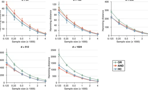
To highlight some of the numerical results, we show in Figures 3.1 and 3.2 the results for the different methods in structure learning experiments with synthetic data. The ground truth graphs had the number of nodes ranging from 64 from 1024 with the corresponding number of edges ranging from 78 to 1248. The inverse of covariance was randomly created with the zero pattern implied by the graph, and the data was sampled from the multivariate normal distribution determined by the inverse of covariance. Figure 3.1 shows the comparison ofAN D graph of FMPL and the `1-based methods. We can see that generally, the AND method performs the best with NBS on tail. Figure 3.2 shows the comparison between the different graphs outputted by FMPL method. We can see thatHCandAN Dgraphs perform quite similarly, while theOR graph does a good job in the settings with less variables (where the true graph is relatively denser).

(30)

20 3 Learning undirected graphical models Sample size (x 1000) 0.125 0.25 0.5 1 2 4 Hamming distance 0 20 40 60 80 100 d = 64 Sample size (x 1000) 0.125 0.25 0.5 1 2 4 Hamming distance 0 40 80 120 160 200 d = 128 Sample size (x 1000) 0.125 0.25 0.5 1 2 4 Hamming distance 0 80 160 240 320 400 d = 256 Sample size (x 1000) 0.125 0.25 0.5 1 2 4 Hamming distance 0 140 280 420 560 700 d = 512 Sample size (x 1000) 0.125 0.25 0.5 1 2 4 Hamming distance 0 260 520 780 1040 1300 d = 1024 AND glasso NBS space

Figure 3.1: Hamming distance with different sample sizes in the structure learning experiments with synthetic data for FMPL and `1-methods. Here, AND graph represents the output of our proposed method. Figure reprinted from Article I.

When the Markov blanket searches were run on a standard 2.3 GHz workstation without utilizing parallelization, the running time of finding all the FMPL graphs ranged roughly from half a second, in case with d= 64 variables, to couple minutes in d= 1024 case.

3.2 Learning non-parametric graphical models

We continue under the theme of learning undirected graphical models. We will present a method for learning undirected graph structures without assuming any particular distribution the data should follow. In order to do this, we will first review some concepts from information theory and try to motivate why the Gaussian assumption might not always be suitable. 3.2.1 Going beyond Gaussian

In the last section our main underlying modeling assumption was that the data follows a multivariate normal distribution. This allowed us to derive a scoring function which was efficient to evaluate even for a high number

(31)

3.2 Learning non-parametric graphical models 21 Sample size (x 1000) 0.125 0.25 0.5 1 2 4 Hamming distance 0 10 20 30 40 50 d = 64 Sample size (x 1000) 0.125 0.25 0.5 1 2 4 Hamming distance 0 20 40 60 80 100 120 d = 128 Sample size (x 1000) 0.125 0.25 0.5 1 2 4 Hamming distance 0 100 200 300 400 d = 256 Sample size (x 1000) 0.125 0.25 0.5 1 2 4 Hamming distance 0 200 400 600 800 d = 512 Sample size (x 1000) 0.125 0.25 0.5 1 2 4 Hamming distance 0 500 1000 1500 2000 2500 d = 1024 OR AND HC

Figure 3.2: Hamming distance with different sample sizes in the structure learning experiments with synthetic data for different FMPL graphs. Figure reprinted from Article I.

of variables. However, assumption that our data follows a multivariate Gaussian distribution is quite rigid, and puts some constraints on the types of relationships between the variables we can model. To be more specific, by assuming normality, the task of deciding whether two variables are independent given some others reduces to testing whether the partial correlation between them is non-zero. As the correlation measures only the strength of a linear relationship, we might not to be able to detect dependencies correctly if the relationships are more complex than linear or if data deviates strongly from Gaussian distribution.

One class of methods that try to deal with this, while still retaining the Gaussian assumption partly, go under the nameGaussian copulas or

non-paranormal methods [33, 34]. The main idea is to find univariate

transformations for each variable so that after the transformation the data can be taken to follow multivariate normal distribution. The transformed data can be then dealt with using any method developed for the Gaussian data.

Kernel methods (see, for instance, [65]) are a second example of methods that are applicable in this situation. Their approach consists roughly of mapping the data to some possibly infinite dimensional space where the

(32)

representation of data allows one to detect complex relationships among the variables.

Our proposed solution to tackle with this problem will use mutual information to devise a non-parametric independence test which can be then paired with a constraint-based structure learning algorithm.

3.2.2 Mutual information and its estimation

Mutual informationI(X, Y) [9] measures the information that a random variable X carries from some other variable Y. For two continuous random variables with joint density pXY(x, y), it is defined as follows:

I(X, Y) = Z x∈X Z y∈Y pXY(x, y) log pXY(x, y) pX(x)pY(y) dxdy, (3.7)

wherepX andpY denote the marginal densities of the corresponding random variables. As a measure of association, mutual information is not restricted to detecting mere linear relationships like correlation. Mutual information equals zero if and only if the variables are independent.

However, estimating mutual information based on observed samples of

XandY might prove tricky in the general case, since if blindly following the definition, we would first need to estimate the densities appearing in (3.7). To bypass this, we will make use of the non-parametric mutual information estimator by Kraskov et al. [28] which relies on the kth-nearest neighbor statistics computed from the observed data.

The Kraskov estimator is based on a previous entropy estimator from Kozachenko and Leonenko [27] which estimates the entropy using the as-sumption that the probability density is constant inside the hyperspheres containing the k−1 nearest neighbors of each data point. The resulting formula for entropy involves distances from each data point to theirkth near-est neighbors. As mutual information is expressible through (differential) entropies, denoted H(·), as

I(X, Y) =H(X) +H(Y)−H(X, Y), (3.8) Kraskov et al. apply the estimator to each of entropies appearing in Eq. (3.8) while taking into account that the length scales in joint and marginal

spaces might be different, effectively canceling the aforementioned distance terms. After finding the kth nearest neighbor of each point (xi, yi) in the joint space and recording the corresponding distancei, the Kraskov mutual information estimator takes the form

b I(X, Y) =ψ(n) +ψ(k)− 1 n n X i=1 [ψ(nx(i) + 1) +ψ(ny(i) + 1)], (3.9)

(33)

3.2 Learning non-parametric graphical models 23 whereψ(·) denotes the digamma function, nis the sample size and nx(i) stands for the number of points found around xi in the marginal space of

X within the distance i (and ny is defined similarly). The choice of the value fork is connected to bias-variance trade-off, as smallerk means that the assumption of constant density is made in smaller volumes.

As our ultimate interest will be to apply the estimator for structure learning, we need to measure association between random variables given the values of some other variables. To this end, we will need conditional mutual informationI(X, Y |Z). An important property regarding independence testing is that conditional mutual information is zero if the variables in question are conditionally independent, specifically

I(X, Y |Z) = 0 if and only ifX⊥⊥Y |Z.

Conditional mutual information also admits a decomposition through en-tropies which makes it possible to estimate it with similar techniques as used in ordinary Kraskov estimator. A formula resembling Eq. (3.9) for computing the conditional mutual information,Ib(X, Y |Z), is provided by

Vejmelka and Paluˇs [61]. Similarly to Eq. (3.9), computing the conditional mutual information requires performing the nearest neighbor search first in the joint space (X, Y, Z), and then counting points inside given radii in the marginal spaces.

3.2.3 Permutation test for conditional independence

While computing the value for conditional mutual informationIb(X, Y |Z)

proved to be straightforward, applying it to independence testing poses another challenge. Even if the random variables under consideration are conditionally independent, the estimatorIb(X, Y |Z) generally never equals

exactly zero due to random fluctuations.

If we knew the distribution of conditional mutual information estimator under the hypothesis of independence, we could just check where the ob-served value lands and use this to guide us when deciding on independence. However, to our best knowledge, the analytical form of the distribution of the estimator still remains elusive, and we need to resort to other means.

To cope with this problem, we will use a permutation test. Given the observed data of size n denoted x = (x1, . . . , xn), y = (y1, . . . , yn) and z = (z1, . . . , zn), we try to simulate the conditional independence by randomly permuting the samplesy and thus breaking the dependence betweenX andY. The idea is to repeatedly permute the dataT times, and compute mutual information Ib(X, Y |Z) using the permuted data. This

(34)

gives us T new different values for mutual information. Using these, we can compare where the initially estimated value ranks among them. Denoting by

K the number of permuted values that exceed the initial value, we get the following estimate for thep-value under the null hypothesis of independence:

ˆ

p= 1 +K 1 +T .

This value can be then compared to predetermined significance level α in order to decide on the independence. This gives us our non-parametric test for conditional independence.

Regarding the computational complexity of mutual information based independence testing, although the permutation test can be done completely in parallel, the single conditional mutual information estimations require nearest neighbor searches that can get computationally demanding as the number of samplesn, or the dimension (through adding more conditioning variables) gets large. The brute force approach would scale as O(kdn2), wheredrefers to the dimension of (X, Y, Z) space. Using data structures such askd-trees [1] one can bring the complexity with respect to the sample size down toO(nlogn).

In our implementation, we also included simple heuristic rules-of-thumb that determine couple situations when the permutation could be skipped and independence deduced. For instance, if fast-to-perform partial correlation based test accepts independence, and estimated conditional mutual infor-mation is below 0.001 nats, we accept the independence without performing the test. For more details, we refer to Sec. 2.3. in Article II.

Even though the permutation test described above breaks the dependence between yand xas desired, Runge [46] notes that this also results in the dependence between permutedy and conditioningz being broken which is in principle wrong when testing for conditional independence. He proposes a local permutation scheme to counter this. This approach involves defining neighborhoods for each data point inZ space, and then permutingylocally with help of these neighborhoods. This introduces an additional tunable hyperparameter,kperm, defining the number of points in the neighborhood. We ran some experiments comparing local permutation scheme to the simple one and found out that local permutation strategy did not seem to result in a more accurate structure recovery when accompanied with the algorithm discussed in the next section. Therefore, we opt to use the simple permutation scheme. For details, we refer to Appendix A of Article II.

(35)

3.2 Learning non-parametric graphical models 25 3.2.4 Empirical performance

To test the method in practice in structure learning, we need to accompany it with a constraint-based learning algorithm. Our strategy will resemble the first step of FMPL algorithm in the last section. That is, we use a constraint-based algorithm to learn the Markov blankets of each variable which we will then combine using theAN D-rule, also described when discussing FMPL, to form the final undirected graph.

To learn the Markov blankets for each node, we use IAMB (incremental association Markov Blanket) algorithm [58]. The algorithm consists of two phases where in the first we add variables to the blanket if they are found to be conditionally dependent given the current blanket. Order in which variables are considered to be added is determined by a dynamic heuristic which in case of our non-parametric test will be the conditional mutual information. In the second phase, we try to identify the possible false positives by removing the nodes that are found to be conditionally independent given the remaining blanket.

The resulting method is referred to as knnMI. Next, we will briefly describe some of the results from experiments in Article II.

We will compare knnMI with k= 5 to other independence tests paired with the same structure learning algorithm. These tests include: Fisher-Z

test for partial correlation (assumes Gaussian data, see, for instance, Kalisch and B¨uhlmann [22]), KCIT [65] which is a non-parametric kernel based method, and RCIT [53], also a kernel method but based on approximations in order to make the test more scalable. Significance level was set toα= 0.05 for every test. In addition to these, we include also the familiar glasso and NBS methods which are applied to data after performing a non-paranormal transformation. These methods are referred to as NPN glasso and NPN mb, respectively.

In the experiments, our main interest was to study how the different methods react when the data generating mechanism deviates from the simple linear Gaussian structure. To that end, we created a data from a small network containing seven nodes and eight edges. To ease the data generation, the graph was selected to be chordal, meaning that we can represent it equally well using a DAG or an undirected graph. We used the DAG form, as it allows us to sample data for each variable given the values of its parents, and varied the following properties in the data generating mechanism:

1. Each variableXiwas defined either as alinear or anon-linear function of its parent variables plus an additive noise term, denoted i. The

(36)

used non-linearities included, for instance, trigonometric functions, logarithm, and absolute value.

2. The additive noise distribution was taken to be either standard Gaus-sian, uniformly distributed between [−1,1], or standard t with two degrees of freedom.

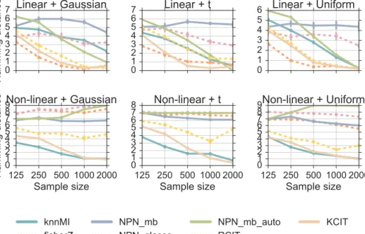
Considering all the options for noise distributions in linear and non-linear settings yields six different scenarios. The results of applying aforementioned structure learning methods to these data sets with different sample sizes are presented in Figure 3.3. The goodness of the learned structures was measured using Hamming distance.

By looking at Figure 3.3, we can see that in the linear case (top-row), kernel methods and the Gaussian test are the most accurate. The proposed method knnMI seems to converge to the right graph but with a slower pace than the leading methods. However, we observe drastic difference in results when we change the relationships in the generating model to be non-linear. In this case (the bottom-row of Figure 3.3) knnMI is generally the best in capturing the underlying structure. KCIT is the runner-up while the other methods do not seem to be able to converge to the right structure.

We considered also a larger version of the non-linear data generating structure. The larger version was created by combining three seven node networks discussed above to create a network with 21 variables. The conclusion from this experiment was the same: knnMI and KCIT were the only methods that seemed to work consistently, knnMI slightly better with small sample sizes.

In addition to this, the methods were tested with non-paranormal data. The data was generated from a Gaussian undirected graphical model with 10 or 20 nodes, and then put through a power transformation. The non-paranormal methods were the best in the larger setting. The exact kernel method KCIT worked also well in these settings and the performance of knnMI was comparable to KCIT with the smallest and the largest sample sizes considered.

To summarize, our method was found to outperform the other methods in case the data generating mechanism involved non-linearities. Out of the tested methods, only the kernel method KCIT could achieve comparable performance in these settings. Comparison of computational complexities for these two methods favors knnMI as the KCIT scales cubicly in the sample size. That being said, all the other compared methods scale better to larger data sets. But as seen in the experiments, the gain in speed might come with a trade-off in accuracy.

(37)

3.2 Learning non-parametric graphical models 27 0 1 2 3 4 5 6 7 Hamming distance Linear + Gaussian 0 1 2 3 4 5 6 7 Linear + t 0 1 2 3 4 5 6 Linear + Uniform 125 250 500 1000 2000 Sample size 0 1 2 3 4 5 6 7 8 9 Hamming distance Non-linear + Gaussian 125 250 500 1000 2000 Sample size 0 1 2 3 4 5 6 7 8 Non-linear + t 125 250 500 1000 2000 Sample size 0 1 2 3 4 5 6 7 8 9Non-linear + Uniform knnMI

fisherZ NPN_mbNPN_glasso NPN_mb_autoRCIT KCIT

Figure 3.3: Structure learning with data generated using linear (top-row) and non-linear (bottom-row) relationships with additive noise (columns). Figure reprinted from Article II.

(38)

(39)

Chapter 4 Learning and applying directed

graphical models

In this chapter, we change our setting in two major ways: 1) we consider discrete random variables instead of continuous, 2) the graphical models we study are directed, Bayesian networks. We start by going through some common scoring criteria that are used when learning Bayesian network struc-tures, and then propose a new one, called Quotient Normalized Maximum Likelihood (qNML). After discussing qNML and its properties, we move on to an application of Bayesian networks. To that end, we review the concept of Fisher kernel and show how it can be combined with Bayesian networks to produce a similarity measure for categorical data vectors.

4.1 Scoring criteria for structure learning in the

discrete setting

LetXdenote an×ddata matrix consisting ofnobservations ondcategorical variables X = (X1, . . . , Xd). Recall from Chapter 2, that the Bayesian network consists of DAGGand parameters θijk =P(Xi =k|Xπ(i) =j). Recall also that Bayesian network allows us to express the likelihood function (see Eq. (2.4)) givenn i.i.d. data pointsX as

p(X |G, θ) = d Y i=1 qi Y j=1 ri Y k=1 θNijk ijk , (4.1)

whereNijk denotes the number of times we observe Xi taking valuek when its parentsXπ(i) take value j in our dataX.

All the scoring functions we consider next are decomposable. Recall that this means we can express them as a sum (or a product) of local scoring

(40)

30 4 Learning and applying directed graphical models

functions: f(G,X) =P

ifi(Xi |Xπ(i)), where the local terms depend only on the data through variableXi and its parents Xπ(i).

4.1.1 BDeu

As we have already seen in Chapter 3, one common choice for f(G,X) is to consider the posterior probability of the graph given the observed data,

p(G|X), which simplifies to marginal likelihood, assuming uniform prior over different graphs.

In the discrete setting, assuming parameter sets θij follow independent Dirichlet distributions,θij ∼Dir(αij1, . . . , αijri), allows one to evaluate the

marginal likelihood in closed form. The resulting score is called Bayesian-Dirichlet-score (BD) [18]. BD-score requires the user to specify hyperpa-rameters αijk which might not be straightforward. A very widely used form of BD-score, called Bayesian-Diriclet equivalence uniform (BDeu), tries to solve this by requiring the user to provide only one tuning parameter: the equivalent sample size, α > 0. Using this, the hyperparameters are set toαijk=α/(riqi). BDeu-score is also score equivalent. This property guarantees that two Bayesian networks G1 andG2 that imply exactly the same assertions of independence, are scored equally.

Even though depending only on one hyperparameter, the BDeu-score can be really sensitive with respect of this choice: in [50], it is shown how the highest scoring DAG structure can vary even from an empty graph to the full network only by changing the value ofα.

Another shortcoming of BDeu was noted by Suzuki [54]. Suzuki shows how BDeu violates regularity in model selection. A decomposable scoring functionfi(Xi |Xπ(i)) is said not to be regular if it prefers a larger parent set over a smaller one, even though the larger set does not provide a better fit to data. The fit to data is here defined via empirical conditional entropy

H(Xi |Xπ(i)), with the smaller entropy implying a better fit. The example in [54] where BDeu violates the regularity involves deterministic relationships between the variables. In [55], it is also argued that regular scores are more efficient when applied with branch-and-bound type search algorithms for structure learning.

4.1.2 BIC

Another very popular scoring function is Bayesian Information Criterion (BIC), which is derived as an asymptotic expansion of the log marginal

(41)

4.1 Scoring criteria for structure learning in the discrete setting 31 likelihood. For the Bayesian networks, it admits the following form:

BIC(G,X) = d X i=1 log ˆp(Xi|Xπ(i))− ki 2 logn, (4.2) where log ˆp(Xi |Xπ(i)) = maxθilogp(Xi |Xπ(i), θi) denotes the maximized

log-likelihood function forXi given the parents Xπ(i), andki=qi(ri−1) is the number of free parameters in the conditional distribution of Xi.

BIC is often stated to have tendency to underfit, preferring simple models unless a lot of data is available. This behaviour is observed for instance in [51], where BIC requires large sample sizes before converging to the correct structure.

4.1.3 fNML

The factorized Normalized Maximum Likelihood (fNML) [51] is a close relative to the qNML criterion that we will present in the next section. Both of these criteria draw their motivation from information theory as they are approximations to a normalized maximum likelihood (NML) criterion which itself is an instance of a more general MDL principle.

Utilizing the NML for learning a Bayesian network structure requires us to compute the NML distribution under any given DAGG defined as

pN M L(X |G) = p(X |G,θˆ(X)) P X0_∈Xp(X0 |G,θˆ(X0)) = Qd i=1pˆ(Xi |Xπ(i)) P X0_∈XQd_i₌₁pˆ(X_i0 |X_π0₍_i₎) , (4.3) where X represents the set off all possible n×d data matrices for our variables X. We have also used notation ˆθ(·) to make the data set from which the maximum likelihood parameters are computed explicit. Taking a log of (4.3) and comparing the result to BIC formula (4.2) shows a clear resemblance, the only difference being the penalty term.

The logarithm of the penalty term, that is, the denominator in (4.3) is calledparametric complexity or regret. This huge sum does not admit a simple factorization over variables, and for a general Bayesian network structure, this term is impossible to compute in reasonable time. However, in case of n observations on a single categorical variable Xi, the regret

reg(n, ri) = logPX0

i∈Xipˆ(X

0

i) and therefore the NML distribution, can be computed efficiently with an exact, linear time (with respect ton andri) algorithm [26] or by constant time approximations [56, 57]. Both, the fNML and the soon-to-be-presented qNML make use of these results.