The weak aggregating algorithm and weak mixability
✩Yuri Kalnishkan
∗, Michael V. Vyugin
Department of Computer Science and Computer Learning Research Centre, Royal Holloway, University of London, Egham, Surrey, TW20 0EX, United Kingdom
Received 10 July 2006; received in revised form 15 June 2007 Available online 29 August 2007
Abstract
This paper resolves the problem of predicting as well as the best expert up to an additive term of the ordero(n), wherenis the length of a sequence of letters from a finite alphabet. We call the games that permit this weakly mixable and give a geometrical characterisation of the class of weakly mixable games. Weak mixability turns out to be equivalent to convexity of the finite part of the set of superpredictions. For bounded games we introduce the Weak Aggregating Algorithm that allows us to obtain additive terms of the formC√n.
©2007 Elsevier Inc. All rights reserved.
Keywords:On-line learning; Predicting individual sequences; Prediction with expert advice; General loss functions
1. Introduction
This paper deals with the problem of prediction with expert advice. We consider the on-line prediction protocol, where outcomesω1, ω2, . . . occur in succession while a prediction strategy tries to predict them. Before seeing an eventωt, the prediction strategy produces a predictionγt. We are interested in the case of a finite outcome space, i.e.,
ω1, ω2, . . .∈Ω such that|Ω|<+∞.
We use a loss functionλ(ω, γ )to measure the discrepancies between predictions and outcomes. A loss function and a prediction space (a set of possible predictions) Γ specify the game, i.e., a particular prediction environment. The performance of a learnerSw.r.t. a game is measured by the cumulative loss
LossS(n)=
n
t=1
λ(ωt, γt) (1)
suffered on a sequence of outcomesω1, ω2, . . . , ωn. In the problem of prediction with expert advice the learner has
access to predictions generated by ‘experts’E1,E2, . . . ,ENthat try to predict elements of the same sequence. The goal
✩ The previous versions of this paper were published as Technical Report CLRC-TR-03-01, Computer Learning Research Centre, Royal
Holloway, University of London (November 2003) and in: Learning Theory, Proceedings of the 18th Annual Conference, COLT 2005, in: Lecture Notes in Artificial Intelligence, vol. 3559, Springer, 2005.
* Corresponding author.
E-mail addresses:[email protected] (Y. Kalnishkan), [email protected] (M.V. Vyugin). 0022-0000/$ – see front matter ©2007 Elsevier Inc. All rights reserved.
of the learner is to predict nearly as well as the best expert, i.e., to suffer loss that is only little bigger than the smallest of the experts’ losses.
This problem has been studied intensively; see, e.g., [1,2] and the overview in the recently published book [3]. Papers [4,5] propose the Aggregating Algorithm that allows the learnerMto achieve loss satisfying the inequality
LossM(n)cLossEi(n)+alnN (2) for alli=1, . . . , N andn=1,2, . . ., where the constantscanda are optimal and are specified by the game. Note that neithercnoradepend onn.
If we can takecequal to 1, the game is called mixable. It is possible to provide a geometrical characterisation of mixable games in terms of the so-called sets of superpredictions. The Aggregating Algorithm fully resolves the problem of predicting as well as the best expert up to an additive constant. For the sake of completeness we formulate one of the results concerning the Aggregating Algorithm in Section 2.4.
There are interesting games that are not mixable, e.g., the absolute loss game introduced in Section 2.1. The Aggregating Algorithm still works for some of such games, but it allows us to achieve only values ofcgreater than 1. In this paper we take a different approach to non-mixable games. We fixc=1 but considera(n)that can grow when the lengthnof the sequence increases. We study the problem of predicting as well as the best expert up too(n)as
n→ +∞, wherenis the length of the sequence. Section 3 introduces the corresponding concept of weak mixability. The main result of this paper, Theorem 7, shows that weak mixability is equivalent to a very simple geometric property of the set of superpredictions, namely, the convexity of its finite part.
If the loss function is bounded, it is possible to predict as well as the best expert up to an additive term of the form
C√n, provided the finite part of the set of superpredictions is convex. This result follows from a recent paper [6]. We shall present our own construction, which is independent of [6] and goes back to ideas from [1]. We develop the Weak Aggregating Algorithm based on the old method of averaging experts’ losses with dynamically updated weights. Unlike the Aggregating Algorithm, which uses the average logβ(
ipiβli), the Weak Aggregating Algorithm uses
simple convex combinationsipili (see Remark 19 for a more detailed discussion); however the way of updating
weights is more complicated.
In [6] (see Remark ‘Deterministic prediction and absolute loss’ at the end of Section 9 in [6]) a result similar to Corollary 14 was obtained. The algorithm used in [6] is based on the ‘following the perturbed leader’ idea while ours belongs to the family of ‘weighted majority’-type algorithms. The extra term obtained in [6], Theorem 6.ii has the multiplicative constant 2√2 as compared to our 2. On the other hand, the analysis in [6] is much more general; some of the bounds obtained there have extra terms depending on the loss of experts rather than time. Those bounds make sense even when the experts’ loss is small, while ours is meaningful only for big losses.
Different algorithms and results leading to various extra terms are widely discussed in the literature; for an overview see [3], Chapter 2 including bibliographic remarks in 2.12. The general question of lower bounds for additive terms of the type considered in this paper remains open. The authors derive some lower bounds in [7] (that paper deals with predictive complexity, but the results can be easily restated for the problem of prediction with expert advice) but the bounds are not sufficiently tight.
If the game is not bounded, our construction can be applied in a different form to predict as well as the best expert up too(n). The result for unbounded games as well as the negative result for games that are not convex constitute the most original contribution of the paper (Appendix A shows that there are indeed unbounded games that are convex but not mixable).
The question of lower bounds for the additive term for unbounded games remains open too.
2. Preliminaries
We will formulate the definitions below without a reference to computability. The negative results of this paper are true in this strong sense. The positive results are proved constructively and algorithms are presented. Therefore the theory can be reformulated in a constructive fashion; see Section 7 for details.
2.1. On-line prediction
AgameGis a tripleΩ, Γ, λ, whereΩ is anoutcome space,Γ is aprediction space, andλ:Ω×Γ → [0,+∞]
ω(0), ω(1), . . . , ω(M−1). In the simplest binary caseM=2 andΩ may be identified withB= {0,1}. We also assume
thatΓ is a compact topological space andλis continuous w.r.t. the extended topology of[−∞,+∞]. Since we treat Ω as a discrete space, the continuity ofλin two arguments is the same as continuity in the second argument. These assumptions hold throughout the paper except for Remark 8, where negative losses are discussed.
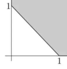
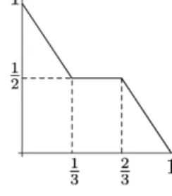
Thesquare-lossgame, theabsolute-lossgame, and thelogarithmicgame with the outcome spaceΩ=B, prediction spaceΓ = [0,1], and loss functionsλ(ω, γ )=(ω−γ )2,λ(ω, γ )= |ω−γ|, and
λ(ω, γ )=
−log2(1−γ ) ifω=0,
−log2γ ifω=1,
respectively, are examples of (binary) games. A slightly different example is provided by thesimple prediction game withΩ=Γ =B= {0,1}andλ(ω, γ )=0 ifω=γ andλ(ω, γ )=1 otherwise.
A gameG= Ω, Γ, λisboundedif and only ifλis bounded, i.e., there isL∈(0,+∞)such thatλ(ω, γ )Lfor eachω∈Ω andγ ∈Γ. If a game is not bounded, we shall call itunbounded. Examples of bounded games include the square-loss game, the absolute-loss game, and the simple prediction game. The logarithmic game is unbounded.
It is essential to allowλto assume the value+∞; this assumption is necessary in order to take into account the logarithmic game as well as other unbounded games. However we impose the following restriction: ifλ(ω0, γ0)= +∞ for someω0∈Ωandγ0∈Γ, then there is a sequenceγn∈Γ such thatγn→γ0andλ(ω, γn)is finite for allω∈Ω
and all positive integers n (note that λ(ω0, γn)→ +∞by continuity). In other words, any prediction that leads
to infinite loss on some outcomes can be approximated by predictions that can only lead to finite loss no matter what outcome occurs. This restriction allows us to exclude some degenerate cases and to simplify the statements of theorems.
2.2. Expert advice
A merging strategy works in an on-line fashion. On trialt it reads predictions of expertsE(1),E(2), . . . ,E(N )and outputs its own. Afterωt, the outcome of trialt, becomes available, the experts and the merging strategy suffer losses.
We want the merging strategy to compete with the experts in terms of the cumulative loss. The goal of the merging strategy is to suffer loss that is not much worse than the loss of the best expert. By the best expert after trialtwe mean the expert that has suffered the smallest cumulative loss so far.
Formally amerging strategyMforN expertsis a function
M:
+∞
t=1
Ωt−1×ΓNt→Γ. (3)
Consider the following on-line protocol: (1) FOR t=1,2, . . .
(2) M reads predictions γt(1), γt(2), . . . , γt(N )∈Γ
(3) M chooses γt ∈Γ
(4) M observes the actual outcome ωt∈Ω
(5) END FOR
By definition, let the total loss ofMafterntrials be
LossGM(n)=
n
t=1
λ(ωt, γt)
and the total loss of expertEi be LossGE i(n)= n t=1 λωt, γt(i) ,
where i=1,2, . . . , N. The upper index Gcan be omitted when it is clear from the context which game we are referring to.
Fig. 1. The square-loss game. Fig. 2. The absolute-loss game.
Fig. 3. The simple prediction game. Fig. 4. The logarithmic game.
One may think of the predictions γt(1), γt(2), . . . , γt(N ) as output by experts E1,E2, . . . ,EN. Note that the term ‘expert’ is only a convenient metaphor. In fact we have a full information game between two parties. Our adversary generates predictionsγt(1), γt(2), . . . , γt(N )∈Γ and outcomesωtwhile we generate predictionsγt. When we say below
that a certain inequality for the total loss of the merging strategy is guaranteed, we mean that it holds no matter what experts’ predictions and outcomes are generated by the adversary.
2.3. Geometric interpretation of a game
Take a gameG= Ω, Γ, λsuch thatΩ= {ω(0), ω(1), . . . , ω(M−1)}and|Ω| =M. The following important defi-nition goes back to [4,5].
Definition 1.AnM-tuple(s0, s1, . . . , sM−1)∈ [0,+∞]M is asuperpredictionif there isγ∈Γ such that the inequal-itiesλ(ω(i), γ )si hold for everyi=0,1,2, . . . , M−1.
The set of superpredictionsSis an important object characterising the game. Figures 1–4 show the sets of super-predictions for the sample binary games defined in Section 2.1.
2.4. Mixability
In this subsection we formulate the result concerning prediction with expert advice for the so-called mixable games. It will not be used in our proofs, but it is important for the motivation.
Take a gameG= Ω, Γ, λsuch thatΩ = {ω(0), ω(1), . . . , ω(M−1)}and|Ω| =M. LetS⊆ [0,+∞]M be its set of superpredictions. Take aβ∈(0,1)and consider the homeomorphismBβ:[0,+∞]M→ [0,1]M specified by the
formulaBβ((x0, x1, . . . , xM−1))=(βx0, βx1, . . . , βxM−1). We can now give the following definition (after [4,5]).
Definition 2.We say thatGisβ-mixable, whereβ∈(0,1), if the setBβ(S)is convex. IfGisβ-mixable for some
β∈(0,1), we say that it ismixable.
For mixable games and only for them we can predict as well as the best expert up to an additive constant; the result can be achieved by a merging strategy following the Aggregating Algorithm (AA).1
1 The Aggregating Algorithm as well as the Weak Aggregating Algorithm introduced in this paper leave some flexibility in the choice of the actual predictions; that is the reason why we do not call them merging strategies in the strict sense.
Fig. 5. The loss λ(ω(0), γ ) for the example from Remark 5.
Fig. 6. The loss λ(ω(1), γ ) for the example from Remark 5.
Proposition 3.(See[4,5].) For every gameG= Ω, Γ, λ
(i) ifGisβ-mixable for someβ∈(0,1), then for everyN=1,2, . . .and for every merging strategyMforNexperts that follows the Aggregating Algorithm, the bound
LossM(n)LossE(i)(n)+ lnN
ln(1/β)
is guaranteed for alln=1,2, . . .and alli=1,2, . . . , N;
(ii) if there is a merging strategyMfor two experts and a positive constantasuch that the inequality LossM(n)LossE(i)(n)+a
is guaranteed for alln=1,2, . . .andi=1,2, thenGis mixable.
If fact, the results concerning the AA hold for a wider class of games with infinite sets of outcomesΩ. The AA can also be shown to be optimal: the constants it achieves in the upper bounds are optimal.
It can be easily shown directly that the square-loss and the logarithmic games are mixable while the absolute-loss and the simple prediction games are not. This is also implied by more general Lemmas 16 and 17 from Appendix A. 2.5. Convexity
Take a gameG= Ω, Γ, λsuch thatΩ= {ω(0), ω(1), . . . , ω(M−1)}and|Ω| =M. LetS⊆ [0,+∞]M be its set of superpredictions. Let us give the following geometrical definition.
Definition 4.We say thatGisconvexif the finite partS∩RM of its set of superpredictionsSis convex.
Remark 5. Suppose thatΓ is a convex set. Then convexity of all the functionsλ(ω(i), γ ),i=0,1, . . . , M−1, in the second argument implies convexity of the game. However the opposite is not true. Indeed, consider a binary game withΓ = [0,1]and the loss function specified by Figs. 5 and 6. Its set of superpredictions coincides with that of the absolute-loss game (Fig. 2), but its loss function is not convex in the second argument.
All mixable games are convex, while the opposite is not true. For example, the absolute-loss game is convex but not mixable. A discussion of convexity and mixability and more examples can be found in Appendix A. The simple prediction game provides an example of a non-convex game.
3. Weak mixability
For non-mixable games it is not possible to predict as well as the best expert up to an additive constant. Let us relax this requirement and ask whether it is possible to predict as well as the best expert up to a larger term.
In the worst case, loss grows linearly in the length of the sequence. Therefore all terms of slower growth can be considered small as compared to loss. This motivates the following definition.
Definition 6.A gameGisweakly mixableif there is a merging strategyMfor two experts and a functionf:N→R (hereN= {1,2, . . .}is the set of positive integers) such thatf (n)=o(n)asn→ +∞and the bound
LossG
M(n)Loss G
E(i)(n)+f (n) (4)
is guaranteed for everyn=1,2, . . .andi=1,2.
We can give an equivalent definition requiring that for everyN =1,2,3, . . .there is a merging strategyMforN
experts such that the inequality LossGM(n)Loss
G
E(i)(n)+f (n)lnN (5)
is guaranteed for alln=1,2, . . .and fori=1,2, . . . , N.
Indeed, a strategy merging two experts can be turned into a strategy mergingN experts by means of the following trick. Let us split the pool of experts into pairs and merge the two experts’ predictions inside each pair. Then we can iterate the procedure until we merge all experts’ predictions into one. (Note that functionsf (n)in the two definitions are different because iterative merging incurs overheads.)
In fact, we shall obtain stronger bounds below. The extra term in the upper bound for the Weak Aggregating Algorithm grows inN asO(√lnN )(see Corollary 14).
The following theorem is the main result of the paper.
Theorem 7.A gameG= Ω, Γ, λis weakly mixable if and only if it is convex, i.e., the finite partS∩RM of the set of superpredictionsSis convex.
Examples of weakly mixable games are the logarithmic and the square-loss game, which are also mixable, and the absolute-loss game, which is not mixable. The simple prediction game is not weakly mixable.
The rest of the paper contains the proof of the theorem. The ‘only if’ part follows from Theorem 9 that is formulated in Section 4 and proved in Appendix B.
The ‘if’ splits into two parts, for bounded and for unbounded games. The ‘if’ part for bounded games follows from [6]. In Section 5 we shall give an alternative derivation, which achieves a slightly better value of the constantCin the additive termC√n. The unbounded case is described in Section 6.
Remark 8.Let us allow (within this remark)λto assume negative values; they can be interpreted as ‘gain’ or ‘reward.’ Ifλassumes the value−∞, the expression for the total loss may include the sum(−∞)+(+∞), which is undefined. In order to avoid this ambiguity, it is natural to prohibitλto take the value−∞. Sinceλis assumed to be continuous andΓ compact, this implies thatλis bounded from below, i.e., there isa >−∞such thatλ(ω, γ )a for all values ofωandγ.
Consider another game with the loss functionλ(ω, γ )=λ(ω, γ )−a, which is non-negative. A merging strategy working with non-negative loss functions can be easily adapted to work with the original game: let the learner just imagine that it is playing the game withλ. The losses w.r.t. the two games on a stringω1ω2. . . ωnwill differ by the
termanand the upper bounds of the type (4) will be preserved. On the other hand, the sets of superpredictions for the two games will differ by a shift, which preserves convexity. Therefore Theorem 7 remains true for games with loss functions bounded from below.
4. ‘Only if’ part
We shall derive a statement that is, in fact, slightly stronger than required by Theorem 7.
Theorem 9.If a game G= Ω, Γ, λ,|Ω| =M <+∞, has the set of superpredictions S such that its finite part
S∩RM is not convex, then there are sequences of experts’ predictionsγt(1)∈Γ and γt(2)∈Γ,t=1,2, . . ., and a constantθ >0such that for any merging strategySfor two experts there is a sequenceωt∈Ω,t=1,2, . . ., such
that max i=1,2 LossGS(n)−LossGE i(n) θ n (6)
For the proof see Appendix B.
5. ‘If’ part for bounded games 5.1. Weak Aggregating Algorithm
In this subsection we introduce the Weak Aggregating Algorithm (WAA). LetG= Ω, Γ, λbe a game such that |Ω| =M <+∞and letN be the number of experts. LetΩ= {ω(0), ω(1), . . . , ω(M−1)}. Although the WAA can be
applied to any game, the performance results we shall obtain hold only for bounded games, so one may assume that
Gis bounded.
We describe the WAA using pseudo-code. The WAA acceptsNinitial normalised weightsq1, q2, . . . , qN∈ [0,1]
such thatNi=1qi=1 and a positive numbercas parameters. The role ofcis similar to that of the learning rate in the
theory of prediction with expert advice. Letβt=e−c/
√ t,t=1,2, . . . (1) l(i)1 :=0, i=1,2, . . . , N (2) FOR t=1,2, . . . (3) wt(i):=qiβ lt(i) t , i=1,2, . . . , N (4) p(i)t := w (i) t N j=1w (j ) t , i=1,2, . . . , N
(5) read experts’ predictions γt(1), γt(2), . . . , γt(N )
(6) gk:=Nj=1λ(ω(k), γt(j ))p (j )
t , k=0,1, . . . , M−1
(7) output γt∈Γ such that λ(ω(k), γt)gk for all k=0,1, . . . , M−1
(8) observe ωt
(9) lt(i)+1:=lt(i)+λ(ωt, γt(i)), i=1,2, . . . , N
(10) END FOR
The variablelt(i)stores the loss of theith expertE(i), i.e., after trialt we havel(i)t+1=LossG
E(i)(t ). The valuesw
(i) t
are weights assigned to the experts during the work of the algorithm; they depend on the loss suffered by the experts and the initial weightsqi. The valuespt(i)are obtained by normalisingw
(i)
t . Note that from the computational point of
view it is sufficient to have only one set of variablesp(i),i=1,2, . . . , N, one set of variablesw(i),i=1,2, . . . , N, and one set of variables l(i),i=1,2, . . . , N to save memory. The subscriptt has been added in order to simplify referring to these variables in the proofs below.
This algorithm is applicable if the set of superpredictionsShas a convex finite partS∩RM. If this is the case, then the point(g0, g1, . . . , gM−1)belongs toSand thusγt can be found on step (7). The choice ofγt is not necessarily
unique.
Remark 10. Suppose that Γ is a convex set and the functions λ(ω, γ )are convex in the second argument for all
ω∈Ω (cf. Remark 5). Then on step (7) we can takeγt=Nj=1p
(j )
t γ
(j )
t (note that it is not necessarily the only
possible solution).
For bounded games the following lemma holds.
Lemma 11.For everyL >0, every gameG= Ω, Γ, λ such that|Ω|<+∞andλ(ω, γ )Lfor allω∈Ω and
γ ∈Γ and everyN=1,2, . . ., for every merging strategyMforN experts that follows the WAA with initial weights
q1, q2, . . . , qN∈ [0,1]such thatNi=1qi=1andc >0the bound
LossM(n)LossE(i)(n)+ cL2+1 cln 1 qi √ n (7)
is guaranteed for everyn=1,2, . . .and everyi=1,2, . . . , N. The proof of Lemma 11 is given in Appendix C.
Fig. 7. A counterexample for unbounded games in dimension 2.
Remark 12.It is easy to see that the result of Lemma 11 will still hold for a countable pool of expertsE1,E2, . . .. We take weights+∞i=1qi=1; the sums in lines (4) and (6) from the definition of the WAA become infinite but they
clearly converge. The point(g0, g1, . . . , gM−1)clearly belongs toSbecauseSis closed (in fact, convexity is sufficient here; a convex combination of countably many points still belongs to their convex closure; see e.g., Theorem 2.4.1 in [8]).
Remark 13. The WAA belongs to the class of merging strategies that on each step produce a distribution
pt(1), p(t2), . . . , pt(N )and suffer loss bounded by the weighted sum of experts’ lossesNi=1λ(ωt, γt(i))p (i)
t . This means
that WAA can be applied to everybounded game in the following randomised fashion. Let us choose one expert from the pool randomly according to this distribution and output the prediction of that expert. Our expected loss on each step will be bounded by the same weighted sum. Therefore (7) will hold with the left-hand side replaced by
ELossM(n), where the expectationEis taken w.r.t. the internal randomisation. Note that the convexity requirement
becomes unnecessary; introducing the randomisation has essentially the same effect as taking the convex hull of the set of superpredictions.
Let us take equal initial weights q1=q2= · · · =qN=1/N in the WAA. The additive term then reduces to
(cL2+(lnN )/c)√n. Whenc=√lnN /L, this expression reaches its minimum. We get the following corollary.
Corollary 14.Under the conditions of Lemma11, there is a merging strategyMsuch that the bound LossM(n)LossE(i)(n)+2L
√
nlnN
is guaranteed.
6. ‘If’ part for unbounded games 6.1. Counterexample
The WAA can be applied even in the case of an unbounded game; indeed, the only requirement is that the finite part of the set of superpredictionsS is convex. However we cannot guarantee that a reasonable upper bound on the loss of a strategy that uses it will exist. The same applies to any strategy that uses a linear combination in the same fashion as WAA.
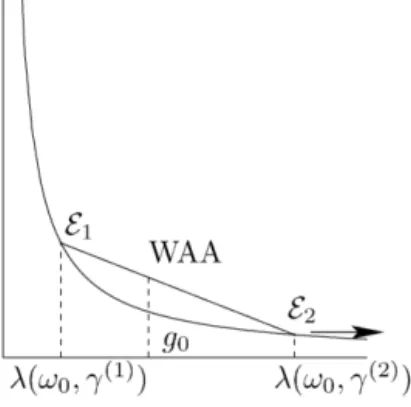
Indeed, consider a game with an unbounded loss function λ. Letω0 be such that the function λ(ω0, γ )attains arbitrary large values.
Suppose that there are two expertsE1andE2and on some trial they are ascribed weightsp(1)andp(2)such that
p(2)>0. Suppose thatE1 outputsγ(1) such thatλ(ω0, γ(1)) <+∞(see Fig. 7 for a two-dimensional illustration). The upper estimate on the loss of the merging strategy in the case when the outcomeω0occurs is
g0=p(1)λ ω0, γ(1) +p(2)λω0, γ(2) ,
Fig. 8. ObtainingLεin the case of two outcomes.
whereγ(2) is the prediction output by E2. Let us vary γ(2). The weights depend on the previous behaviour of the experts and they cannot be changed. Ifλ(ω0, γ(2))tends to infinity, theng0tends to infinity and therefore the difference
g0−λ(ω0, γ(1))tends to infinity. Thus the learner cannot compete with the first expert.
This example shows that the WAA cannot be straightforwardly generalised to unbounded games. It needs to be altered.
6.2. Approximating unbounded games with bounded
The following lemma allows us to ‘cut off’ the infinity at a small cost.
Lemma 15. LetG= Ω, Γ, λ be a game such that |Ω|<+∞. Then for every ε >0 there isLε>0 with the
following property. For every γ∈Γ there isγ∗∈Γ such thatλ(ω, γ∗)Lε andλ(ω, γ∗)λ(ω, γ )+ε for all
ω∈Ω.
The proof of Lemma 15 is given in Appendix D.
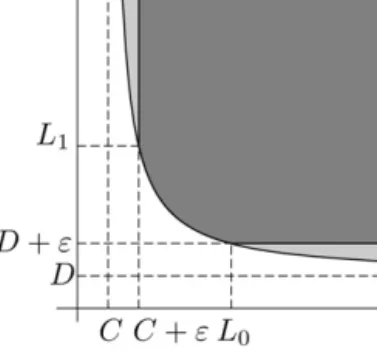
In the case of two outcomes|Ω| =2 obtainingLεis particularly straightforward. See Fig. 8, where
C= inf γ∈Γλ ω(0), γ and D= inf γ∈Γλ ω(1), γ;
we can takeLε=max(L0, L1). Ifγis such that the point(λ(ω(0), γ ), λ(ω(1), γ ))falls into the area to the right of the straight linex=L0, we can takeγ∗such that(λ(ω(0), γ∗), λ(ω(1), γ∗))=(L0, D+ε).
6.3. Merging experts in the unbounded case
Consider an unbounded gameG= Ω, Γ, λandN expertsE1,E2, . . . ,EN. Fix someε >0. LetLε be as above.
After obtaining experts’ predictionsγt(1), γt(2), . . . , γt(N )we can findγt(1)∗, γt(2)∗, . . . , γt(N )∗as in Lemma 15 and then apply the results from the bounded case to them. By proceeding in this fashion, a strategyMsuffers loss such that
LossGM(n)LossGE(i)(n)+Cε
√
n+εn (8)
for all i=1,2, . . . , N andω1, ω2, . . . , ωn∈Ω,n=1,2, . . ., where Cε=2L2ε
√
lnN (we are applying WAA with equal weights).
This inequality does not allow us to prove Theorem 7. In order to achieve an extra term of the ordero(n)we shall varyε.
Take a strictly increasing sequence of integersNk,k=1,2, . . ., and a sequenceεk>0,k=0,1,2, . . .. Consider
the merging strategyMdefined as follows. The strategy first takesε0and merges the experts’ predictions using the WAA andε0in the fashion described above. This continues whilen, the length of the sequence of outcomes, is less than or equal toN1. Then the strategy switches toε1and applies the WAA andε1untilnexceedsN2, etc. (see Fig. 9). Note that each timenpasses through a limitNi, the current invocation of the WAA terminates and a completely new
Fig. 9. The sequences ofNk,Mk, andεk.
In Appendix E we show how to choose the sequencesεkandNkin such a way as to achieve the desired extra term
of the ordero(n).
7. Computability issues
Since the results of this paper are proved constructively, they can be restated in a constructive fashion.
Let us require in Definition 6 thatMis computable. The experts do not have to be computable in any sense because in our analysis the merging strategy has no access to their internal ‘machinery.’ The merging strategy simply receives experts’ predictions as inputs. Note that we can choose computable sequencesγt(1) andγt(2) in Theorem 9 though. The sequenceωncan be generated effectively ifMis computable.
In order for the merging strategies constructed in the proof of Theorem 7 to be computable, we need to impose computability restrictions on games. We require the loss function to be computable so that the operations we need to do become possible.
We need to be able do the following. First we need to compute the values ofλ. Secondly in order to perform step (7) of the WAA we need to be able to solve systems of inequalities of the type
λω(0), γt0, λω(1), γt1, .. . λω(M−1), γtM−1 w.r.t.γ, whereti= m
j=1pjλ(ω(i), γj)for some set ofγjand weightspj(i=0,1, . . . , M−1 andj=1,2, . . . , N).
Note that we only encounter systems where the solution is known to exist. Thirdly for unbounded games we need to compute the valuesLεfrom Lemma 15. If we have the value ofLε, we can findγ∗for everyγ0by solving the system of the aforementioned type withti=min(λ(ω(i), γ0)+ε, Lε),i=0,1, . . . , M−1.
These requirements are quite natural and every reasonable loss function (e.g., specified by a reasonable analytical expression) should satisfy them.
Remark 10 simplifies our task ifΓ is convex andλconvex in the second argument. We can then findγt on step (7)
of the WAA by taking a convex combination onΓ.
Suppose that we have an oracle that can answer the questions of the types we have listed. Then both the WAA and the algorithm for unbounded functions we have constructed output the prediction on each step of the on-line protocol inO(MN )time modulo calls to the oracle.
Acknowledgments
We would like to thank participants of the Kolmogorov seminar on complexity theory at the Moscow State Uni-versity and Alexander Shen in particular for useful suggestions that allowed us to simplify the WAA. We would also like to thank Volodya Vovk for suggesting an idea that helped us to strengthen an upper bound on the performance of WAA.
We are grateful to anonymous COLT and JCSS referees for their detailed comments. The paper has been greatly improved due to referees’ suggestions.
Appendix A. Convexity vs mixability
In this appendix we show that convexity is a weaker requirement than mixability. All mixable games are convex, while the converse is not true. We shall give a geometrical proof and construct examples.
Lemma 16.If a gameG= Ω, Γ, λsuch thatΩ= {ω(0), ω(1), . . . , ω(M−1)}is mixable, then it is convex.
Proof. We shall rely on a characterisation of convexity by means of support hyperplanes (see, e.g., Theorems 8 and 9 in [9]).
Take a point x0=(x0(0), x0(1), . . . , x0(M−1))∈RM on the boundary∂(S∩RM). Letβ∈(0,1)be such that Gis
β-mixable and henceBβ(S)is convex. Through the pointBβ(x0)there passes a support hyperplane toBβ(S).
Because the setBβ(S)contains the whole parallelepiped with the diagonal from the origin toBβ(x0), the equation of the hyperplane can be written as Mi=−01aiu(i)=1, where ai 0 for alli=0,1, . . . , M−1 (hereu(i) are the
coordinates inRM).
Therefore the set Slies ‘above’ the surface passing throughx0and specified by the equationiM=−01aiβx
(i) =1 (herex(i)are the coordinates inRM), whereai0 for alli=0,1, . . . , M−1. Sinceaβx=βx+logβa, this surface is a
shift of either the surfaceMi=−01βx(i)=1 or a cylinder over a similar surface of lower dimension. Since the function
βx is concave, the sumMi=−01βx(i) is concave and the set {(x(0), x(1), . . . , x(M−1))∈RM−1|βx(i)1}is convex. A support hyperplane passes through each point on the surface; thus we can draw a support hyperplane toS∩RM
throughx0. 2
We shall now construct binary examples differentiating convex games from mixable. We need the following lemma from [10] (it is in fact a restatement of results from [2]).
Lemma 17.LetGbe a binary game with the set of superpredictionsS. Suppose that there are twice differentiable functionsx, y:I →R, whereI⊆Ris an open(perhaps infinite)interval, such thatx>0andy<0onI andSis the closure of the set{(u, v)∈R2|there ist∈I:x(t )uandy(t )v}w.r.t. the extended topology of[−∞,+∞]2. Then, for everyβ∈(0,1), the gameGisβ-mixable if and only if
ln1
β
y(t )x(t )−x(t )y(t ) x(t )y(t )(y(t )−x(t ))
holds for everyt∈I. The gameGis mixable if and only if the fraction(yx−xy)/xy(y−x)is separated from the zero, i.e., there isε >0such that
yx−xy
xy(y−x)ε (9)
holds onI.
Proof. Convexity ofBβ(S)is equivalent to concavity of the function with the graph{Bβ(x(t ), y(t ))|t∈I}. Because
the functionsx(t )andy(t )are smooth, this curve is concave if and only if the inequality
d2βy(t ) d(βx(t ))20
holds onI. Differentiation yields
dβy(t ) dβx(t ) =β y(t )−x(t )y(t ) x(t ) and d2βy(t ) d(βx(t ))2= βy(t )−2x(t ) lnβ·(x(t ))2 y(t )−x(t )y(t )lnβ+y (t )x(t )−y(t )x(t ) x(t ) .
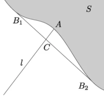
Fig. 10. The drawing for the proof of Theorem 9.
Using this lemma, one can check that the square-loss and the logarithmic games are mixable, while the absolute-loss game is not.
If in the lemmax(t )=t, one can rewrite (9) as
y
y(y−1)ε >0.
The convexity requirement reduces toy0. These formulae allow us to construct various examples of convex games that are not mixable.
If the second derivative ofy(x)vanishes inside the interval (buty(x)does not become constant), theny(x)specifies the set of superpredictions of a non-mixable game.
The following group of examples shows that mixability can be violated ‘at the infinity.’ Let I =(0,+∞)and
y(x)=1/xm,m >0. We have
y y(y−1)=
(m+1)xm m+xm+1
and the fraction tends to 0 asx→0 orx→ +∞. Clearly all the games with the sets of superpredictions specified
by such y(x)are convex and unbounded but not mixable. However if we cut off the ends of the interval and take
I=(a, b), where 0< a < b <+∞, we get mixable games.
Appendix B. Proof of the ‘only if’ part
Proof of Theorem 9. We shall use the following simple vector notation. IfX=(x1, . . . , xn),Y =(y1, . . . , yn)and
α∈R, thenX+Y andαXare defined in the natural way. ByX, Ywe denote the scalar productni=1xiyi. Vector
inequalities, e.g.,XY, hold if they hold component-wise. Note that the definition of the set of superpredictionsS
implies that ifX∈SandYXthanY ∈S.
For brevity we shall denote finite sequences by bold letters, e.g.,x=ω1. . . ωn∈Ωn. Let|x|be the length ofx,
i.e., the total number of symbols inx. We shall denote the number of elements equal toω(0)in a sequencexby0x, the number of elements equal toω(1)by1x, etc. It is easy to see thatiM=−01ix= |x|for everyx∈Ω∗. The vector
(0x, 1x, . . . , M−1x)will be denoted byx.
There are pointsB1=(b1(0), b1(1), . . . , b1(M−1))andB2=(b2(0), b(21), . . . , b2(M−1))such thatB1, B2∈S∩RMbut the segment[B1, B2]connecting them is not a subset ofS. Letα∈(0,1)be such thatC=αB1+(1−α)B2does not belong toS(see Fig. 10). Sinceλis continuous andΓ is compact, the setSis closed and thus there is a small vicinity ofCthat is a subset ofRM\S.
Without restricting the generality one may assume that all coordinates ofB1andB2are strictly positive. Indeed, the pointsB1=B1+t·(1,1, . . . ,1)andB2 =B2+t·(1,1, . . . ,1)belong toSfor all positivet. Ift >0 is sufficiently small, thenC=αB1+(1−α)B2 still belongs to the vicinity mentioned above and thusCdoes not belong toS.
Let us draw a straight linel through the origin and pointC. LetA=(a(0), a(1), . . . , a(M−1))be the intersection oflwith the boundary∂S. Such a point really exists. Indeed,l= {X∈RM| ∃t0: X=t C}. For sufficiently larget
all coordinates oft Care greater than the corresponding coordinates ofB1and thust C∈S. Now lett0=inf{t0|
t C∈S}andA=t0C. SinceC /∈S, we gett0>1 and thusA=(1+δ)C, whereδ >0.
We now proceed to constructing the sequences γt(1) and γt(2). There are predictions γ1, γ2 ∈ Γ such that
λ(ω(i), γ1)b(i)1 andλ(ω(i), γ2)b(i)2 for alli=0,1,2, . . . , M−1. Letγt(1)=γ1andγt(2)=γ2for allt=1,2, . . .. Ifx=ω1ω2. . . , ωt, then LossE1(t ) M−1 i=0 ixb(i)1 = B1, x, (10) LossE2(t ) M−1 i=0 ixb(i)2 = B2, x (11) for allt=1,2, . . ..
Now let us consider a merging strategySand construct a sequencexn=ω1ω2. . . ωnsatisfying the requirements of
the theorem. The sequence is constructed by induction. Suppose thatxnhas been constructed. Letγ be the prediction
output bySon the(n+1)th trial, provided the previous outcomes were elements constituting the stringsxn in the
correct order. There is some ω(i0)∈Ω such thatλ(ω(i0), γ )a(i0). Indeed, if this is not true and the inequalities
λ(ω(i), γ ) < a(i)hold for alli=1,2, . . . , M−1, then there is a vicinity ofAthat is a subset ofS. This contradicts the definition ofA. We letxn+1=xnωi0. The construction implies
LossS(n)
M−1
i=0
ixna(i)= A, xn. (12)
Letε=minj=1,2;i=0,1,2,...,M−1b(i)j >0. We getBj,x =
M−1
i=0 b
(i)
j ixε|x| for all stringsx∈Ω∗ andj =
1,2. SinceA=(1+δ)(αB1+(1−α)B2)we get A, x =(1+δ)αB1, x +(1−α)B2, x
αB1, x +(1−α)B2, x +δε|x|
for all stringsx. Letθ=δε; note thatεandδdo not depend onS. By combining this inequality with (10), (11), and (12) we obtain the inequality
LossS(n)αLossE1(n)+(1−α)LossE2(n)+θ n
for all positive integersn. It is easy to see that
LossS(n)−LossE1(n)(1−α) LossE2(n)−LossE1(n)+θ n, LossS(n)−LossE2(n)α LossE1(n)−LossE2(n)+θ n.
If LossE2(n)LossE1(n)the former difference is greater than or equal toθ n, otherwise the latter difference is greater than or equal toθ n. By combining these two inequalities we obtain (6). 2
Appendix C. Proof of Lemma 11
In this appendix we prove Lemma 11. We start with the following lemma.
Lemma 18.LetG= Ω, Γ, λbe a game such that|Ω|<+∞and let N be the number of experts. Let the finite part of the set of superpredictionsS∩RM be convex. IfMis a merging strategy following the WAA, then for every
t=1,2, . . .we get βLoss G M(t ) t β t j=1δ(j ) t N i=1 qiβ LossG E(i)(t ) t , (13)
where δ(j )=logβj β N i=1λ(ωj,γj(i))p(i)j j N i=1β λ(ωj,γj(i)) j p (i) j (14)
forj =1,2, . . . , t, in the notation introduced above.
Proof. The proof is by induction ont. Let us assume that (13) holds and then derive the corresponding inequality for the stept+1.
The functionxα, where 0< α <1 andx0, is increasing inxand it is also concave inx. For every set of weights
pi ∈ [0,1], i=1, . . . , n such that
n
i=1pi =1 and every array of xi 0, i=1, . . . , n, we get (
n i=1pixi)α n i=1pixiα. Therefore (13) implies βLoss G M(t ) t+1 = βLoss G M(t ) t log βtβt+1 (15) β t j=1δ(j ) t N i=1 qiβ LossG E(i)(t ) t log βtβt+1 (16) β t j=1δ(j ) t+1 N i=1 qiβ LossG E(i)(t ) t+1 . (17)
Step (7) of the algorithm implies thatλ(ωt+1, γt+1) N
i=1λ(ωt+1, γt(i)+1)p(i)t+1. By exponentiating this inequality we get βλ(ωt+1,γt+1) t+1 β N i=1λ(ωt+1,γt(i)+1)p (i) t+1 t+1 (18) = β N i=1λ(ωt+1,γt(i)+1)p (i) t+1 t+1 N i=1β λ(ωt+1,γt(i)+1) t+1 p (i) t+1 N i=1 βλ(ωt+1,γ (i) t+1) t+1 p (i) t+1 (19) =βtδ(t+1+1) N i=1 βλ(ωt+1,γ (i) t+1) t+1 p (i) t+1. (20)
Multiplying (17) by (20) and substituting
pt(i)+1=wt+1 N j=1w (j ) t+1 = qiβ LossG E(i)(t ) t+1 N j=1qjβ LossG E(j )(t ) t+1 completes the proof on the lemma. 2
By taking the logarithm of (13) we get LossGM(t ) t j=1 δ(j )+logβt N i=1 qiβ LossG E(i)(t ) t t j=1
δ(j )+logβtqi+LossGE(i)(t ) for everyi=1,2, . . . , N. We have logβtqi= −
√
t
Recall thatLis an upper bound onλ. By applying the inequality lnxx−1 we get δ(t )= N i=1 λωt, γt(i) p(i)t + √ t c ln N i=1 βλ(ωt,γt(i)) t p (i) t N i=1 λωt, γt(i) p(i)t + √ t c N i=1 βλ(ωt,γ (i) t ) t p (i) t −1 .
By using Taylor’s series with Lagrange’s remainder term we obtain
βλ(ωt,γ (i) t ) t =e−cλ(ωt,γ (i) t )/ √ t= 1−cλ(ωt, γ (i) t ) √ t + 1 2 cλ(ω√t, γt(i)) t 2 eξ, whereξ∈ [−cλ(ωt, γt(i))/ √ t,0]and thus βλ(ωt,γ (i) t ) t 1− cλ(ω√t, γt(i)) t + c2L2 2t .
Thereforeδ(t )cL2/2√tand summation yields
t j=1 δ(j ) t j=1 cL2 2√j cL2 2 t 0 dx √ x =cL 2√t . This completes the proof.
Remark 19.Let us discuss the intuitive meaning of the termδ(t ). We have
δ(t )= N i=1 λωt, γt(i) p(i)t −logβt N i=1 βλ(ωt,γt(i)) t p (i) t .
This is the difference of two terms corresponding to two different ways of mixing experts’ predictions. The first is the convex mixture we use in the WAA. The second is the mixture used in the Aggregating Algorithm (AA) (see [4,5]). In the AA the transformationBβ(see Section 2.4) is applied, a mixture is calculated in the image space, and then the
inverse imageB−β1is taken. This is only possible if the game isβ-mixable, while for the WAA convexity is sufficient. What we have shown is that the loss suffered by the hypothetical AA-style mixture converges to the loss of the convex combination fast enough asβ approaches 1.
Appendix D. Proof of Lemma 15
For everyε >0 andγ∗∈Γ the setU (γ∗, ε)= {γ∈Γ |λ(ω, γ∗) < λ(ω, γ )+εfor allω∈Ω}is open. Indeed,λ
is continuous andU (γ∗, ε)is an intersection of finitely many inverse images of open sets.
For every finiteL >0 letΓL= {γ∈Γ |λ(ω, γ )Lfor allω∈Ω}. Fixε >0. The unionL>0
γ∗∈ΓLU (γ ∗, ε)
is an open covering ofΓ. Indeed, consider someγ0∈Γ. If the valuesλ(ω, γ0)are finite for allω, thenγ0belongs to someΓL. If some of these values are infinite,γ0can still be approximated by predictions that can only lead to finite losses and thereforeγ0belongs toU (γ∗, ε)of some suchγ∗.
SinceΓ is compact, a finite subcovering exists and thus a finiteLcan be chosen. This proves the lemma.
Remark 20.The lemma can also be proven by constructing a covering of the set of superpredictionS. This way is slightly longer, but arguably more intuitive because the construction is done inRM.
Let |Ω| =M and Ω= {ω(0), ω(1), . . . , ω(M−1)}. Let ΓL be as above and consider the sets PL= {(λ(ω(0), γ ),
λ(ω(1), γ ), . . . , λ(ω(M−1), γ ))|γ∈ΓL}.
For everyε >0 letV (L, ε)be theε-vicinity of the setPL, i.e., the union of all open balls of radiusεcentred on
points fromPL. Finally, letS(L, ε)= {X∈ [−∞,+∞]M|XY for someY ∈VL,ε}.
It is easy to check that for every >0 we haveS⊆L>0S(L, ε). One can show that this covering has a finite subcovering by considering the image under the transformationBβ (see Section 2.4) with someβ∈(0,1).
Appendix E. Choosing the sequences
TakeM0=N1andMj=Nj+1−Nj,j=1,2. . .. Let a positive integernbe such thatNk< nNk+1(see Fig. 9). Applying (8) yields
LossGM(n)LossE(i)(n)+r(n)
for alli=1,2, . . . , N, whereNis the number of experts and
r(n)= k−1 j=0 Mjεj+ k−1 j=0 Cεj Mj+εk(n−Nk)+Cεk n−Nk (21)
is the ‘remainder’ (we recall thatCε=2L2ε
√
lnN). Note that the former two terms correspond to the previous invo-cations of WAA and the later two correspond to the current invocation.
We shall formulate conditions sufficient for the terms in (21) to be ofo(n)order of magnitude. First note that (1) limj→+∞εj=0
andk=k(n)→ ∞asn→ ∞is sufficient to ensure thatεk(n−Nk)=o(n)asn→ ∞. Secondly, if, moreover,
(2) ∞j=0Mj= +∞
thenkj−=10Mjεj=o(n)by the following simple lemma.
Lemma 21.If the series∞i=1Mi diverges andαi →0, where allMi andαi are non-negative, then
k
i=1Miαi =
o(ki=1Mi)ask→ ∞.
Proof of Lemma 21. Take a smallε >0. There is positive integerlsuch thatαi< ε/2 for allil. We thus have k i=1 Miαi l i=1 Miαi+ ε 2 k i=l Mi
for allkl. Since the series diverges,ki=lMi tend to+∞ask→ ∞and thus for sufficiently largek l i=1 Miαi ε 2 k i=l Mi and therefore k i=1 Miαiε k i=1 Mi. 2
Thirdly, the lemma implies that if, moreover, (3) Cεj 8 Mj,j=0,1,2, . . ., thenkj−=10Cεj Mjkj−=10Mj/Mj3/8=o(n).
It remains to consider the last term in (21). There are two cases, eithern−NkMk3/4orn−Nk> Mk3/4. In the
former case we get 1 nCεk n−Nk Mk1/8√n−Nk Nk Mk1/8Mk3/8 Mk−1 = √ Mk Mk−1 ,
while in the latter case we get 1 nCεk n−Nk Mk1/8√Mk Mk3/4 = 1 Mk1/8 .
To ensure the convergence to 0, it is sufficient to add (4) Mj−1Mj3/4,j=1,2, . . .
and to replace (2) with a stronger requirement (2) Mj→ +∞,j→ ∞.
Let us show that conditions (1)–(4) are compatible, i.e., construct the sequences εj and Mj. Let M0 = max(2,Cε8
0)andMj+1= M
4/3
j ,j=0,1,2, . . .. The sequenceεj is constructed as follows. Suppose that allεj
have been constructed forjk. IfCεk/2M 1/8
k , we letεk+1=εk/2; otherwise we letεk+1=εk. SinceMk→ +∞
andCεis finite for everyε >0, we shall be able to divideεkby 2 eventually and thus ensure thatεj→0 asj → +∞.
References
[1] N. Cesa-Bianchi, Y. Freund, D. Haussler, D.P. Helmbold, R.E. Schapire, M.K. Warmuth, How to use expert advice, J. ACM 44 (3) (1997) 427–485.
[2] D. Haussler, J. Kivinen, M.K. Warmuth, Sequential prediction of individual sequences under general loss functions, IEEE Trans. Inform. Theory 44 (5) (1998) 1906–1925.
[3] N. Cesa-Bianchi, G. Lugosi, Prediction, Learning, and Games, Cambridge University Press, 2006.
[4] V. Vovk, Aggregating strategies, in: Proceedings of the 3rd Annual Workshop on Computational Learning Theory, Morgan Kaufmann, San Mateo, CA, 1990, pp. 371–383.
[5] V. Vovk, A game of prediction with expert advice, J. Comput. System Sci. 56 (1998) 153–173.
[6] M. Hutter, J. Poland, Adaptive online prediction by following the perturbed leader, J. Mach. Learn. Res. 6 (April 2005) 639–660.
[7] Y. Kalnishkan, M.V. Vyugin, On the absence of predictive complexity for some games, in: Algorithmic Learning Theory, 13th International Conference, Proceedings, in: Lecture Notes in Artificial Intelligence, vol. 2533, Springer, 2002, pp. 164–172.
[8] D. Blackwell, M.A. Girshik, Theory of Games and Statistical Decisions, Wiley, 1954. [9] H.G. Eggleston, Convexity, Cambridge University Press, Cambridge, 1958.
[10] Y. Kalnishkan, M.V. Vyugin, Mixability and the existence of weak complexities, in: Computational Learning Theory, 15th Annual Conference, Proceedings, in: Lecture Notes in Artificial Intelligence, vol. 2375, Springer, 2002, pp. 105–120.