Factoring and Testing
Irreducibility of Sparse
Polynomials over Small
Finite Fields
Richard P. Brent
Australian National University
joint work with
Paul Zimmermann
INRIA, Nancy
France
30 March 2009
Outline
• Introduction– Polynomials over finite fields
– Irreducible and primitive polynomials
– Fermat and Mersenne primes • Part 1: Testing irreducibility
– Irreducibility criteria
– Modular composition
– Three algorithms
– Comparison of the algorithms
– The “best” algorithm
– Some computational results • Part 2: Factoring polynomials
– Distinct degree factorization
– Avoiding GCDs, blocking
– Another level of blocking
– Average-case complexity
– New primitive trinomials
2
Polynomials over finite fields
We consider univariate polynomialsP(x) over a finite fieldF. The algorithms apply, with minor changes, for any small positive characteristic, but since time is limited we assume that the characteristic is two, andF =Z/2Z= GF(2).
P(x) isirreducibleif it has no nontrivial factors. IfP(x) is irreducible of degreer, then [Gauss]
x2r =xmodP(x).
ThusP(x) divides the polynomial Pr(x) =x2
r
−x. In fact,Pr(x) is the product of
all irreducible polynomials of degreed, whered
runs over the divisors ofr.
LetN(d) be the number of irreducible polynomials of degreed. Thus
X
d|r
dN(d) = deg(Pr) = 2r.
By M¨obius inversion we see that
rN(r) =X
d|r
µ(d)2r/d.
Counting irreducible polynomials
Thus, the number of irreducible polynomials of degreeris N(r) = 2 r r +O 2r/2 r ! .Since there are 2rpolynomials of degreer, the probability that a randomly selected polynomial is irreducible is∼1/r→0 asr→+∞. In this sense,almost allpolynomials over (fixed) finite fields are reducible (just as almost all integers are composite).
Analogy. Polynomials of degreerare analogous to prime numbers ofrdigits. By the prime number theorem, the number ofr-digit primes in basebis about Z br br−1 dt lnt= br−br−1 rlnb 1 +O 1 r .
The Riemann Hypothesis implies an error term
O(rbr/2) asr→+∞for the integral on the left [von Koch].
Irreducible and primitive polynomials
Irreducible polynomials over finite fields are useful in several applications. As one example, observe that, ifP(x) is an irreduciblepolynomial of degreer over GF(2), then GF(2)[x]/P(x)∼= GF(2r). In other words, the ring of polynomials modP(x) gives a
representation of the finite field with 2r elements.
If, in addition,xis a generator of the multiplicative group, that is if every nonzero element of GF(2)[x]/P(x) can be represented as a power ofx, thenP(x) is said to beprimitive. Primitive polynomials can be used to obtain linear feedback shift registers (LFSRs) with maximal period.
In general, to test primitivity, we need to know the prime factorization of 2r−1.
The number of primitive polynomials of degree
rover GF(2) is
φ(2r−1)
r ≤N(r),
with equality when 2r−1 is prime.
5
Fermat and Mersenne primes
AFermat primeis a prime of the form 2n+ 1. There areconjecturedto be only finitely many. Forn <233the only examples are
3,5,17,257,65537. Note thatnis necessarily a power of 2, because ifn=pqwithp >1 odd, then 2q+ 1 is a nontrivial divisor of 2n+ 1.
The converse is false, as shown by Euler: 232+ 1 = 641×6700417.
AMersenne primeis a prime of the form 2n−1, for example 3,7,31,127,8191, . . .
There areconjecturedto be infinitely many Mersenne primes. The number forn≤N is conjectured to be of order logN.
The GIMPS project is searching systematically for Mersenne primes. So far 46 Mersenne primes are known, the largest being
243112609−1.
If 2n−1 is prime we say that nis aMersenne exponent. A Mersenne exponent is necessarily prime, but not conversely (211−1 = 23×89).
6
Part 1: Testing irreducibility
Since irreducible polynomials are “rare” but useful, we are interested in algorithms for testing irreducibility.
From [Gauss],P(x) of degreer >1 is irreducible iff
x2r=xmodP(x)
and, for all prime divisorsdofr, we have GCDx2r/d−x, P(x)= 1.
The second condition is required to rule out the possibility thatP(x) is a product of irreducible factors of some degree(s)k=r/d,d|r.
This condition does not significantly change anything, so let us assume thatris prime. (In our examplesris a Mersenne exponent, so necessarily prime.) ThenP(x) is irreducible iff
x2r =xmodP(x).
One more assumption
All the algorithms involve computations mod
P(x), that is, in the ring GF(2)[x]/P(x). In the complexity analysis we assume thatP(x) issparse, that is, the number of nonzero coefficients is small. Thus, reduction of a polynomial modP(x) can be done in linear time. The algorithms to be discussed still work without this assumption, but the complexity analysis no longer applies because more time is spent in the reductions modP(x).
In applicationsP(x) is often atrinomial P(x) =xr+xs+ 1, r > s >0.
Irreducible and primitive trinomials
There is no known formula for the number of irreducible or primitivetrinomialsof degreerover GF(2) (unlike the case of general polynomials).
SinceN(r)≈2r/r, the probability that a
randomly chosen polynomial of degreer will be irreducible is about 1/r. It isplausibleto assume that the same applies to trinomials. There arer−1 trinomials of degreer, so we might expectO(1) of them to be irreducible. More precisely, we might expect a Poisson distribution with some constant meanµ. This plausible argument isfalse, as shown by Swan’s theorem. We state a [corrected] version of Swan’s Corollary 5 that is relevant to trinomials.
Historical note: Swan (1962) rediscovered results of Pellet (1878) and Stickelberger (1897), so the name of the theorem depends on your nationality.
9
Swan’s theorem (Corollary 5)
Theorem 1 Letr > s >0, and assumer+sis odd. ThenTr,s(x) =xr+xs+ 1has an even
number of irreducible factors overGF(2)in the following cases:
a)r even,r6= 2s,rs/2 = 0or1mod4. b)r odd,snot a divisor of2r,r=±3mod8. c)r odd,sdivisor of2r, r=±1mod8. In all other casesxr+xs+ 1has an odd
number of irreducible factors.
If bothr andsare even, thenTr,s(x) is a
square. If bothr andsare odd, apply the theorem toTr,r−s(x).
Forr an odd prime, ignoring the easily-checked casess= 2 orr−s= 2,
case (b) says that the trinomial has aneven number of irreducible factors, and hence must bereducible, ifr=±3 mod 8.
For primer=±1 mod 8, the heuristic Poisson distribution does seem to apply, with mean
µ≈3. Similarly for primitive trinomials, with a correction factorφ(2r−1)/(2r−2).
10
First algorithm — repeated squaring
Our first and simplest algorithm for testing irreducibility is justrepeated squaring:Q(x)←x; forj←1 tordo Q(x)←Q(x)2modP(x); ifQ(x) =xthen returnirreducible else returnreducible.
The operationQ(x)←Q(x)2modP(x) can be performed in timeO(r). The constant factor is small. We recommend the fast squaring algorithm of Brent, Larvala and Zimmermann (2003). This saves both operations and memory references, and is about 2.2 times faster than the obvious squaring algorithm (as implemented in most otherwise-good software packages). Since the irreducibility test involvesr squarings, the overall time isO(r2).
Polynomial multiplication
Before describing other algorithms for irreducibility testing, we digress to discuss polynomial multiplication, matrixmultiplication, and modular composition. To multiply two polynomialsA(x) andB(x) of degree (at most)r, the “classical” algorithm takes timeO(r2). There are faster algorithms, e.g. Karatsuba, Toom-Cook, and FFT-based algorithms.
For polynomials over GF(2), the asymptotically fastest known algorithm is due to Sch¨onhage. (The Sch¨onhage-Strassen algorithm does not work in characteristic 2, and it is not clear whether F¨urer’s ideas are useful here.) Sch¨onhage’s algorithm runs in time
M(r) =O(rlogrlog logr).
In practice, forr≈32 000 000, a multiplication takes about 480 times as long as a squaring.
Matrix multiplication
Letωbe the exponent of matrix multiplication, so we can multiplyn×nmatrices in time
O(nω+ε) for anyε >0. The best result is
Coppersmith and Winograd’sω <2.376, though in practice we would use the classical (ω= 3) or Strassen (ω= log27≈2.807) algorithm. Since we are working over GF(2), our matrices have single-bit entries. This means that the classical algorithm can be implemented very efficiently using full-word operations (32 or 64 bits at a time). Nevertheless, Strassen’s algorithm is faster ifnis larger than about 1000.
Good in practice is the “Four Russians” algorithm [Arlazarov, Dinic, Kronod & Faradzev, 1970]. It computesn×nBoolean matrix multiplication in timeO(n3/logn). We can use the Four Russians’ algorithm up to some threshold, sayn= 1024, and Strassen’s recursion for largern, combining the advantages of both.
13
Modular composition
Themodular compositionproblem is: given polynomialsA(x),B(x),P(x), compute
C(x) =A(B(x)) modP(x).
If max(deg(A),deg(B))< r= deg(P), then we could computeA(B(x)), a polynomial of degree at most (r−1)2, and reduce it moduloP(x). However, this wastes both time and space. Better is to compute
C(x) = X
j≤deg(A)
aj(B(x))j modP(x)
by Horner’s rule, reducing modP(x) as we go, in timeO(rM(r)) and spaceO(r). Using Sch¨onhage’s algorithm for the polynomial multiplications, we can computeC(x) in time
O(r2logrlog logr).
14
Faster modular composition
Using an algorithm of Brent & Kung (1978), based on an idea of Paterson and Stockmeyer, we can reduce the modular composition problem to a problem of matrix multiplication. If the degrees of the polynomials are at mostr, andm=⌈r1/2⌉, then we have to performm multiplications ofm×mmatrices. The matrices are over the same field as the polynomials (that is, GF(2) here). The Brent-Kung modular composition algorithm takes time
O(r(ω+1)/2) +O(r1/2M(r)),
where the first term is for the matrix multiplications and the second term is for computing the relevant matrices.
Assuming Strassen’s matrix multiplication, the first term isO(r1.904) and the second term is
O(r1.5logrlog logr). Thus, the second term is asymptotically negligible (but maybe not in practice).
Using modular composition
Recall that our problem is to computex2r modP(x). Repeated squaring is not the only way to do this.
LetAk(x) =x2
k
modP(x). Then a modular composition algorithm can be used to compute
Ak(Am(x)) modP(x). Since
Ak(Am(x)) = x2
m2k
modP(x) =Am+k(x),
we can computex2r
modP(x) with about log2(r) modular compositions instead ofr squarings.
For example, ifr= 17, we have (all computations in GF(2)[x]/P(x)): A1(x) =x2, (trivial) A2(x) =A1(A1(x)) =x4, (≡1 squaring) A4(x) =A2(A2(x)) =x16, (≡2 squarings) A8(x) =A4(A4(x)) =x256, (≡4 squarings) A16(x) =A8(A8(x)) =x2 16 , (≡8 squarings) A17(x) =A16(x)2=x2 17 , (1 squaring) using only 4 modular composition steps.
Second algorithm
To summarise, we can compute
Ar(x) =x2
r
modP(x) by the following recursive algorithm that uses the binary representation ofr(notthat of 2r):
ifr= 0 then returnx
else ifreven then {U(x)←Ar/2(x);
returnU(U(x)) modP(x)} else
returnAr−1(x)2modP(x). The algorithm takes about log2(r) modular compositions. Hence, if Strassen’s algorithm is used in the Brent-Kung modular composition algorithm, we can test irreducibility in time
O(r1.904logr).
17
Third algorithm
Recently, Kedlaya and Umans (2008) proposed an asymptotically fast modular composition algorithm that runs in timeOε(r1+ε) for any
ε >0.
The algorithm is complicated, involving iterated reductions to multipoint multivariate
polynomial evaluation, multidimensional FFTs, and the Chinese remainder theorem.
See the papers on Umans’s web site
www.cs.caltech.edu/~umans/research.htm
Using the Kedlaya-Umans fast modular composition instead of the Brent-Kung reduction to matrix multiplication, we can test irreducibility in timeOε(r1+ε).
Warning: the “Oε(· · ·)” notation indicates that
the implicit constant depends onε. In this case, it is a rather large and rapidly increasing (probably exponential) function of 1/ε.
18
Comparison of the algorithms
So the last shall be first, and the first lastMatthew 20:16 The theoretical time bounds predict that the third algorithm should be the fastest, and the first algorithm the slowest. However, this is only forsufficiently largedegreesr.
In practice, forr up to at least 4.3×10⁷, the situation is reversed! The first algorithm is the fastest, and the third algorithm is the slowest. A minor drawback of the first (squaring) algorithm is that it is hard to speed up on a parallel machine. The other algorithms are much easier to parallelise. However, this is not so relevant when we are considering many trinomials, as we can let different processors of a parallel machine work on different trinomials in parallel.
Example,
r
= 32 582 657
Following are actual or estimated times on a 2.2 Ghz AMD Opteron 275 forr= 32 582 657 (a Mersenne exponent).
1. Squaring (actual): 64 hours 2. Brent-Kung (estimates):
• classical: 265 hours (19% mm) • Strassen: 254 hours (15% mm) • Four Russians: 239 hours (10% mm)
(plus Strassen forn >1024) 3. Kedlaya-Umans (estimate): >1010years The Brent-Kung algorithm would be the fastest if the matrix multiplication were dominant; unfortunately theO(r1/2M(r)) overhead term dominates.
Since the overhead scales roughly asr1.5, we estimate that the Brent-Kung algorithm would be faster than the squaring algorithm for
Note on Kedlaya-Umans
´Eric Schost writes:
The Kedlaya-Umans algorithm reduces modular composition to the multipoint evaluation of a
multivariate polynomial, assuming the base field is large enough.
The input of the evaluation is overFp; the algorithm works overZ
and reduces modpin the end. The evaluation overZis done by CRT modulo a bunch of smaller primes, and so on. At the end-point of the recursion, we do a naive evaluation on all ofFpm, wherepis the current prime andmthe number of
variables. So the cost here is≥pm. [Now he considers choices ofmin the caser= 32 582 657; all give
pm≥1.36×1027.]
Our estimate of>1010years is based on a time of 1 nsec per evaluation (very optimistic).
21
The “best” algorithm
Comparing the second algorithm with the first, observe that the modular compositions do not all save equal numbers of squarings. In fact the lastmodular composition saves⌊r/2⌋squarings, thesecond-lastsaves⌊r/4⌋squarings, etc. Each modular composition has the same cost. Thus, if we can use only one modular
composition,it should be the one that saves the most squarings.
If we use⌊r/2⌋squarings to compute
x2⌊r/2⌋
modP(x), then use one modular composition (and one further squaring, ifr is odd), we can computex2r modP(x) faster than with any of the algorithms considered so far, providedrexceeds a certain threshold.
In the example, the time would be reduced from 64 hours to 44 hours, a saving of 31%.
Doing two modular compositions would reduce the time to 40 hours, a saving of 37%.
22
Computational results
In 2007-8 Paul Zimmermann and I conducted a search for irreducible trinomialsxr+xs+ 1 whose degreeris a (known) Mersenne exponent. Since 2r−1 is prime,irreducible
impliesprimitive. The previous record degree of a primitive trinomial wasr= 6 972 593.
r s
24 036 583 8 412 642, 8 785 528
25 964 951 880 890, 4 627 670, 4 830 131, 6 383 880 30 402 457 2 162 059
32 582 657 5 110 722, 5 552 421, 7 545 455 Table 1: Ten new primitive trinomialsxr+xs+ 1
of degree a Mersenne exponent, fors≤r/2. We used the first algorithm to test irreducibility of the most difficult cases. Most of the time was spent discarding the vast majority of trinomials that have a small factor, using a new factoring algorithm with good average-case behaviour (the topic of the second half of this talk).
Part 2: Factoring
The problem of factoring a univariate polynomialP(x) over a finite fieldF often arises in computational algebra. An important case is whenF has small characteristic and
P(x) has high degree but issparse(has only a small number of nonzero terms).
Since time is limited, I will make the same assumptions as in Part 1: F= GF(2) and
P(x) is sparse, typically a trinomial
P(x) =xr+xs+ 1, r > s >0,
although the ideas apply more generally. The aim is to give an algorithm with good amortized complexity, that is, one that works wellon average. Since we are restricting attention to trinomials, we average over all trinomials of fixed degreer.
Equivalently, we can use probabilistic language, and assume a uniform distribution over all trinomials of fixed degreer.
Distinct degree factorization
I will only considerdistinct degree factorization. That is, ifP(x) has several factors of the same degreed, the algorithm will produce the product of these factors. The
Cantor-Zassenhaus algorithm can be used to split this product into distinct factors. This is usually cheap because in most cases the product has small degree or consists of just one factor.
Factor of smallest degree
To simplify the complexity analysis and speed up the algorithm in the common application of searching for irreducible polynomials, I only consider the time required to findonenontrivial factor (it will be a factor of smallest degree) or output “irreducible”.
Certificates of reducibility
A nontrivial factor (preferably of smallest degree) gives a “reducibility certificate” that can quickly be checked.
25
Factorization in
GF(2)[
x
]
From now on we write “+” instead of “−” (they are equivalent in GF(2)[x]).
As we already mentioned,x2d+xis the product of all irreducible polynomials of degree
dividingd. For example,
x23+x=x(x+ 1)(x3+x+ 1)(x3+x2+ 1).
Thus, a simple (but slow) algorithm to find a factor of smallest degree ofP(x) is to compute GCD(x2d
+x, P(x)) ford= 1,2, . . .. The first time that the GCD is nontrivial, it contains a factor of minimal degreed. If the GCD has degree> d, it must be a product of factors of degreed.
If no factor has been found ford≤r/2, where
r= deg(P(x)), then P(x) must be irreducible. Note thatx2d
should not be computed explicitly; instead computex2dmodP(x) by repeated squaring.
26
Application to trinomials
Some simplifications are possible whenP(x) =xr+xs+ 1 is a trinomial.
• We can skip the cased= 1 because a trinomial can not have a factor of degree 1.
• SincexrP(1/x) =xr+xr−s+ 1, we only need considers≤r/2.
• By applying Swan’s theorem, we can usually show that the trinomial under consideration has an odd number of factors; in this case we only need check
d≤r/3.
Complexity of squares and muls
In Part 1 we already considered the complexity of computing squares and products inGF(2)[x]/P(x). Recall that, with our usual assumption thatP(x) is sparse, squaring can be performed in time
S(r) = Θ(r)≪M(r)
and multiplication can be performed in time
M(r) =O(rlogrlog logr).
In the complexity estimates we assume that
M(r) is a sufficiently smooth and well-behaved function.
Complexity of GCD
For GCDs we use a sub-quadratic algorithm that runs in timeG(r) =O(M(r) logr). More precisely,
G(2r) = 2G(r) +O(M(r)),
so
M(r) =O(rlogrlog logr)⇒G(r) = Θ(M(r) logr).
In practice, forr≈2.4×10⁷ and our implementation on a 2.2 Ghz Opteron, S(r)≈0.005 seconds, M(r)≈2 seconds, G(r)≈80 seconds, M(r)/S(r)≈400, G(r)/M(r)≈40. 29
Avoiding GCD computations
In the context of integer factorization,Pollard (1975) suggested a blocking strategy to avoid most GCD computations and thus reduce the amortized cost; von zur Gathen and Shoup (1992) applied the same idea to polynomial factorization.
The idea of blocking is to choose a parameter
ℓ >0 and, instead of computing
GCD(x2d+x, P(x)) for d∈[d′, d′+ℓ),
compute
GCD(pℓ(x2
d′
, x), P(x)),
where theinterval polynomialpℓ(X, x) is
defined by pℓ(X, x) = ℓY−1 j=0 X2j+x .
In this way we replaceℓGCDs by one GCD and
ℓ−1 multiplications modP(x). 30
Backtracking
The drawback of blocking is that we may have to backtrack ifP(x) has more than one factor with degrees in [d′, d′+ℓ), soℓshould not be
too large. The optimal strategy depends on the expected size distribution of factors and the ratio of times for GCDs and multiplications.
New idea - multi-level blocking
We introduce a finer level of blocking to replace most multiplications by squarings, which speeds up the computation in GF(2)[x]/P(x) of the interval polynomialspm(x2d, x), where
pm(X, x) = mY−1 j=0 X2j+x= m X j=0 xm−jsj,m(X), sj,m(X) = X 0≤k<2m, w(k)=j Xk,
andw(k) denotes the Hamming weight ofk. Note thatsj,m(X2) =sj,m(X)2 in
GF(2)[x]/P(x). Thus,pm(x2
d
, x) can be computed with costm2S(r) if we already know
sj,m(x2
d−m
) for 0< j ≤m.
In this way we replacemmultiplications andm
squarings by one multiplication andm2 squarings. Choosingm≈pM(r)/S(r) (about 20 ifM(r)/S(r)≈400), the speedup over single-level blocking is aboutm/2≈10.
Fast initialization
The polynomials sj,m(x) = X 0≤k<2m, w(k)=j xksatisfy a “Pascal triangle” recurrence relation
sj,m(x) =sj,m−1(x2) +x×sj−1,m−1(x2) with boundary conditions
sj,m(x) = 0 if j > m ,
s0,m(x) = 1.
Thus, we can compute
{sj,m(x) modP(x) | 0≤j≤m}
in timeO(m2r), even though the definition of
sj,m(x) involvesO(2m) terms.
Question: Have the polynomialssj,m(x) been
studied before? It seems probable but I have not found any references to them.
33
Recapitulation
To summarize, we use two levels of blocking: • The outer level replaces most GCDs by
multiplications.
• The inner level replaces most multiplications by squarings. • The blocking parameter
m≈pM(r)/S(r) is used for the inner level of blocking.
• A different parameterℓ=kmis used for the outer level of blocking.
34
Example
Figure 1: ℓ= 15,m= 5 In the example,S= 1/25,M= 1,G= 10 No blocking: cost 15G+ 15S= 150.6 1-level blocking: G+ 14M+ 15S= 24.6 2-level blocking: G+ 2M+ 75S= 15.0 More realistically, supposeℓ= 80,m= 20,S= 1/400,M= 1,G= 40
No blocking: cost 80G+ 80S= 3200.2 1-level blocking: G+ 79M+ 80S= 119.2 2-level blocking: G+ 3M+ 1600S= 47.0
Sieving
Asmallfactor is one with degreed <1 2log2r, so 2d<√r.
It would be inefficient to find small factors in the same way as large factors. Instead, let
d′= 2d−1,r′=rmodd′,s′=smodd′. Then
P(x) =xr+xs+ 1 =xr′
+xs′
+ 1 mod (xd′
−1),
so we only need compute
GCD(xr′+xs′+ 1, xd′−1).
The cost of finding small factors is negligible (both theoretically and in practice), so will be ignored.
In the definition, the fraction 12 is rather arbitrary; it can be replaced by 1−ε for any
Distribution of degrees of factors
In order to predict the expected behaviour of our algorithm, we need to know the expected distribution of degrees of irreducible factors. Our complexity estimates here are based on the assumption that trinomials of degreer behave like the set of all polynomials of the same degree, up to a constant factor:Assumption 1 Over all trinomialsxr+xs+ 1
of degreer overGF(2), the probabilityπdthat a
trinomial has no nontrivial factor of degree≤d is at mostc/d, wherec is a constant and 1< d≤r.
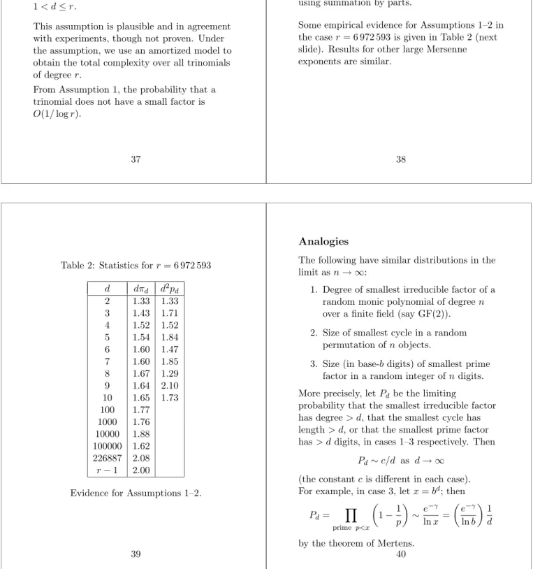
This assumption is plausible and in agreement with experiments, though not proven. Under the assumption, we use an amortized model to obtain the total complexity over all trinomials of degreer.
From Assumption 1, the probability that a trinomial does not have a small factor is
O(1/logr).
37
Simpler approximation
Letpd=πd−1−πdbe the probability that the
smallest nontrivial factor of a randomly chosen trinomial has degreed≥2. Although not strictly correct, the following is a good approximation.
Assumption 2 pdis of order1/d2, providedd
is not too large.
I will use Assumption 2 because it simplifies the amortized complexity analysis, but the same results can be obtained from Assumption 1 using summation by parts.
Some empirical evidence for Assumptions 1–2 in the caser= 6 972 593 is given in Table 2 (next slide). Results for other large Mersenne exponents are similar.
38
Table 2: Statistics forr= 6 972 593
d dπd d2pd 2 1.33 1.33 3 1.43 1.71 4 1.52 1.52 5 1.54 1.84 6 1.60 1.47 7 1.60 1.85 8 1.67 1.29 9 1.64 2.10 10 1.65 1.73 100 1.77 1000 1.76 10000 1.88 100000 1.62 226887 2.08 r−1 2.00
Evidence for Assumptions 1–2.
Analogies
The following have similar distributions in the limit asn→ ∞:
1. Degree of smallest irreducible factor of a random monic polynomial of degreen
over a finite field (say GF(2)). 2. Size of smallest cycle in a random
permutation ofnobjects.
3. Size (in base-bdigits) of smallest prime factor in a random integer ofndigits. More precisely, letPdbe the limiting
probability that the smallest irreducible factor has degree> d, that the smallest cycle has length> d, or that the smallest prime factor has> ddigits, in cases 1–3 respectively. Then
Pd∼c/d as d→ ∞
(the constantcis different in each case). For example, in case 3, letx=bd; then
Pd= Y prime p<x 1−1 p ∼ e −γ lnx = e−γ lnb 1 d
Outer level blocking strategy
The blocksize in the outer level of blocking is
ℓ=km. We take an increasing sequence
k=k0j for j= 1,2,3, . . . ,
wherek0mis of order logr (since small factors will have been found by sieving). This leads to a quadratic polynomial for the interval bounds. There is nothing magic about a quadratic polynomial, but it is simple to implement and experiments show that it is reasonably close to optimal.
Using the data that we have obtained on the distribution of degrees of smallest factors of trinomials, and assuming that this distribution is insensitive to the degreer, we could obtain a strategy that is close to optimal. However, the choicek0jwith suitablek0is simple and not too far from optimal. The number of GCD and sqr/mul operations is usually within a factor of 1.5 of the minimum possible.
41
Expected cost of sqr/mul
Recall that the inner level of blocking replaces
mmultiplications bym2squarings and one multiplication, wherem≈pM(r)/S(r) makes the cost of squarings about equal to the cost of multiplications.
For a smallest factor of degreed, the expected number of squarings ism(d+O(√d)). Averaging over all trinomials of degreer, the expected number is O m X d≤r/2 d+O(√d) d2 =O(mlogr) .
Thus, the expected cost of sqr/mul operations per trinomial is
OS(r) logrpM(r)/S(r) = OlogrpM(r)S(r) = Or(logr)3/2(log logr)1/2 .
42
Expected cost of GCDs
Suppose thatP(x) has smallest factor of degreed. The number of GCDs required to find the factor, using our (quadratic polynomial) blocking strategy, isO(√d). By Assumption 2, the expected number of GCDs for a trinomial with no small factor is
1 +O X (lgr)/2<d≤r/2 √ d d2 = 1 +O 1 √ logr .
Thus the expected cost of GCDs per trinomial is
O(G(r)/logr) =O(M(r)) =O(rlogrlog logr).
This is asymptotically≪expected cost of sqr/mul operations
In practice, forr≈4.3×10⁷, GCDs take about 65% of the time versus 35% for sqr/mul. Once again, the asymptotic analysis is misleading, because the function
s logr
log logr
is a very slowly growing function ofr.
Comparison with classical algorithms
For simplicity I will use theOenotation which ignores log factors.The “classical” algorithm takes an expected timeOe(r2) per trinomial, orOe(r3) to cover all trinomials of degreer.
The new algorithm takes expected timeOe(r) per trinomial, orOe(r2) to cover all trinomials of degreer.
In practice, the new algorithm is faster by a factor of about 160 forr= 6 972 593, and by a factor of about 1000 forr= 43 112 609. Thus, comparing the computation for
r= 43 112 609 with that forr= 6 972 593: using the classical algorithm would take about 240 times longer (impractical), but using the new algorithm saves a factor of 1000.
Generally, our search for different Mersenne exponentsr∈ {6 972 593, 24 036 583, 25 964 951, 30 402 457, 32 582 657, 43 112 609}took less time for largerr, due to incremental improvements in the search program!
Recent computational results
Since Sept 2008 we have been searching for primitive trinomials of degree 43 112 609 (the largest known Mersenne exponent).Dan Bernstein and Tanja Lange have joined in the search and contributed CPU cycles. So far we completed about 98% of the search and found four new primitive trinomials
xr+xs+ 1,r= 43 112 609:
s= 3 569 337, 4 463 337, 17 212 521, 21 078 848 Testing irreducibility took about 119 hours per trinomial on a 2.2 Ghz AMD Opteron, using our first algorithm. The “best” algorithm would take about 69 hours (saving 42%).
Most of the time (about 22 processor-years) was spent eliminating reducible trinomials at an average rate of about 32 sec per trinomial (×43112609/2 trinomials).
45
Conclusion
The new double-blocking strategy works well and, combined with fast multiplication and GCD algorithms, has allowed us to find new primitive trinomials of record degree. This would have been impractical using the classical algorithms.
The same ideas work over finite fields GF(p) for small primep >2, and for factoring sparse polynomialsP(x) that are not necessarily trinomials: all we need is that the time forp-th powers (modP(x)) is much less than the time for multiplication (modP(x)).
46
Acknowledgement
Thanks to ´Eric Schost for his comments on the work of Kedlaya and Umans; to Dan Bernstein and Tanja Lange for contributing computer time to the search for degree 43 112 609; to Alan Steel for independently verifying our new primitive trinomials using Magma; and to Victor Shoup for his package NTL, which was used to debug our software and check our certificates.
References
[1] V. L. Arlazarov, E. A. Dinic, M. A. Kronod & I. A. Faradzev, On economical construction of the transitive closure of an oriented graph,Soviet Math. Dokl.11
(1975), 1209–1210.
[2] W. Bosma & J. Cannon,Handbook of Magma Functions, School of Mathematics and Statistics, University of Sydney, 1995.
http://magma.maths.usyd.edu.au/
[3] R. P. Brent, P. Gaudry, E. Thom´e & P. Zimmermann, Faster multiplication in GF(2)[x],Proc. ANTS VIII 2008,Lecture Notes in Computer Science5011, 153–166.
http://wwwmaths.anu.edu.au/~brent/ pub/pub232.html
[4] R. P. Brent & H. T. Kung, Fast algorithms for manipulating formal power series,J. ACM25(1978), 581–595.
.../pub045.html
[5] R. P. Brent, S. Larvala & P. Zimmermann, A fast algorithm for testing reducibility of trinomials mod 2 and some new primitive trinomials of degree 3021377,Math. Comp. 72(2003), 1443–1452..../pub199.html
[6] R. P. Brent & P. Zimmermann, A multi-level blocking distinct-degree factorization algorithm,Finite Fields and Applications: Contemporary Mathematics 461(2008), 47–58..../pub230.html
[7] R. P. Brent & P. Zimmermann, Ten new primitive binary trinomials,Math. Comp. 78(2009), 1197–1199..../pub233.html
[8] D. G. Cantor and H. Zassenhaus, A new algorithm for factoring polynomials over finite fields,Math. Comp.36(1981), 587–592.
[9] D. Coppersmith & W. Winograd, Matrix multiplication via arithmetic progressions, J. Symb. Comput.9(1980), 251–280. [10] M. F¨urer, Faster integer multiplication,
Proc. 48th STOC Conference, 2007, 57–66. [11] J. von zur Gathen & J. Gerhard,Modern
Computer Algebra, Cambridge Univ. Press, 1999.
[12] J. von zur Gathen and J. Gerhard, Polynomial factorization overF2,Math.
Comp.71(2002), 1677–1698.
49
[13] J. von zur Gathen and V. Shoup,
Computing Frobenius maps and factoring polynomials,Computational Complexity 2
(1992), 187–224.
http://www.shoup.net/papers/
[14] K. Kedlaya & C. Umans, Fast modular composition in any characteristic,Proc. FOCS 2008, 146–155.http://www.cs. caltech.edu/~umans/research.htm
[15] T. Kumada, H. Leeb, Y. Kurita and M. Matsumoto, New primitivet-nomials (t= 3, 5) over GF(2) whose degree is a Mersenne exponent,Math. Comp.69
(2000), 811–814. Corrigenda: ibid71
(2002), 1337–1338.
[16] A.-E. Pellet, Sur la d´ecomposition d’une fonction enti`ere en facteurs irr´eductibles suivant un module premierp,Comptes Rendus de l’Acad´emie des Sciences Paris 86(1878), 1071–1072.
[17] J. M. Pollard. A Monte Carlo method for factorization,BIT15(1975), 331–334,
50
[18] A. Sch¨onhage, Schnelle Multiplikation von Polynomen ¨uber K¨orpern der
Charakteristik 2,Acta Inf.7(1977), 395–398.
[19] ´E. Schost,Fast irreducibility test, personal communication, 4 June 2008.
[20] V. Shoup, NTL: A library for doing number theory.http:www.shoup.net/ntl/
[21] L. Stickelberger, ¨Uber eine neue Eigenschaft der Diskriminanten
algebraischer Zahlk¨orper,Verhandlungen des ersten Internationalen Mathematiker-Kongresses, Z¨urich, 1897, 182–193. [22] R. G. Swan, Factorization of polynomials
over finite fields,Pacific J. Math.12
(1962), 1099–1106.
[23] G. Woltmanet al, GIMPS, The Great Internet Mersenne Prime Search.