Explainable NILM Networks

(1)

Explainable NILM Networks

David Murray, Lina Stankovic, Vladimir Stankovic

[email protected],[email protected],[email protected] University of Strathclyde

Glasgow, United Kingdom

ABSTRACT

There has been an explosion in the literature recently on Non-intrusive load monitoring (NILM) approaches based on neural net-works and other advanced machine learning methods. However, though these methods provide competitive accuracy, the inner workings of these models is less clear. Understanding the outputs of the networks help in improving the designs, highlights the relevant features and aspects of the data used for making the decision, pro-vides a better picture of the accuracy of the models (since a single accuracy number is often insufficient), and also inherently provides a level of trust in the value of the provided consumption feedback to the NILM end-user. Explainable Artificial Intelligence (XAI) aims to address this issue by explaining these “black-boxes”. XAI methods, developed for image and text-based methods, can in many cases interpret well the outputs of complex models, making them trans-parent. However, explaining time-series data inference remains a challenge. In this paper, we show how some XAI-based approaches can be used to explain NILM deep learning-based autoencoders inner workings, and examine why the network performs or does not perform well in certain cases.

CCS CONCEPTS

•Computing methodologies→Neural networks;Feature se-lection.

KEYWORDS

neural networks, explainable artificial intelligence (XAI), inter-pretable machine learning

ACM Reference Format:

David Murray, Lina Stankovic, Vladimir Stankovic. 2020. Explainable NILM Networks. InThe 5th International Workshop on Non-Intrusive Load Moni-toring (NILM’20), November 18, 2020, Virtual Event, Japan.ACM, New York,

NY, USA, 6 pages. https://doi.org/10.1145/3427771.3427855

1 INTRODUCTION

Deep learning models have become significantly larger than that of 10 years ago and with the ability to transfer trained model layers, un-derstanding how the network is trained and how it can be adapted

Permission to make digital or hard copies of all or part of this work for personal or classroom use is granted without fee provided that copies are not made or distributed for profit or commercial advantage and that copies bear this notice and the full citation on the first page. Copyrights for components of this work owned by others than ACM must be honored. Abstracting with credit is permitted. To copy otherwise, or republish, to post on servers or to redistribute to lists, requires prior specific permission and/or a fee. Request permissions from [email protected].

NILM’20, November 18, 2020, Virtual Event, Japan

to a new use case has become increasingly more important [5]. Ex-amples of this would be the use and modification of ResNet [6] by Microsoft, GoogLeNet [20] by Google and AlexNet [10] where pre-trained image classification models can be downloaded and with minimal changes to input and output layers, image classification re-sults can be obtained on a new dataset which are on par to the state of the art [11]. More recently, the AlphaGo Zero network which, given only the basic rules of play of the Chinese game Go, has taught itself how to play Go at the highest level starting from a totally random play [19]. As these types of reinforcement network and the deep pre-trained networks are finding applications in critical sys-tems, such as self driving cars, police, space, and other exploration missions, the need to understand their inner-working and interpret the decisions the system makes, are increasingly important. Thus, the field of Explainable Artificial Intelligence (XAI) [4] [3] [12] [2] has become the focus of research interest lately, mainly evolving around developing models that are interpretable-by-design or de-veloping “post-hoc” algorithms that can interpret “black boxes” such as deep learning-based models [1] [14]. Another driver for the XAI research is the recent EU legislation that empowers a cus-tomer to request explanations for AI system decisions, recital 71 of the EU GDPR law [17]. Examples of network explainability can be seen in well-known image networks [1] [14]. With the addition of saliency maps and attention mechanisms it is possible to see what the network is ‘looking at’ when it is classifying images which can be important to make sure that the network is not learning ‘data noise’ or a common feature in images, e.g., classifying the blue background as a fish instead of the fish in the foreground.

Deep Learning has become a major staple of recent NILM work with about a third of papers published last year mentioning neural networks in some form or another [7] [23] [9] [21] [25], [16]. In many cases these networks attain state-of-the-art results in event detection and regression tasks [8] [26]. However, it is unclear what the network has learned in terms of pattern recognition, or indeed if it has been over-trained for the given example house or dataset. Furthermore, it is unclear what kind of features the network looks for, and consequently, if and when a pre-trained model can be used on unseen houses [16]. Averaged accuracy results very often misrepresent the learning ability of the network, and can give the wrong impression on what to expect on a case by case basis.

Models are becoming more complex and being able to under-stand how a network learns can allow for accuracy improvement via improved architecture designs and hyper-parameter selection and also better transparency, especially if the model is providing NILM results to utility customers, where incorrect information will be questioned as it may led to disadvantaging the customer and providing them misleading energy saving advice.

(2)

Since deep learning models are becoming more involved, provid-ing “post-hoc" interpretability is becomprovid-ing an increasprovid-ingly challeng-ing task. In this paper, we study interpretability of deep learnchalleng-ing models for non-intrusive load monitoring (NILM) and how inter-pretability can help improve the performance.

2 AUTOENCODER MODEL

To exemplify explainable NILM, we use an one-dimensional autoen-coder model, which takes the aggregate signal as an input and the appliance signal as an output. The architecture is suitable for the NILM problem as it reconstructs the appliance power signal making it easier to calculate the consumed power, rather than classifying it, if the appliance is on or off. This provides a better indication of how much an appliance actually consumed instead of estimating the average power consumption from detected edges, e.g., from event-based approaches.

The network is initially trained to recreate the aggregate input signal to learn feature representations. The model has the decoder reset and is trained to represent a single appliance type using the features it has learned from the aggregate signal. In particular, the model consists of 9 layers, 4 encoding convolutional layers, 4 decod-ing layers and an output layer, each with ReLU activation. We used two dropout layers, after the first two encoding layers. The input is a window size of 2048 samples at 10sec sampling rate (downsam-pled from 8s). Training involved preprocessing and normalising both aggregate and appliance signals to a range between 0 and 1. This was done by a min/max scaler where the aggregate signal was set to a maximum of 12,000W and the appliance signal to a maximum of 3000W. In extreme use cases where the aggregate is higher than 12,000 Watts the values would be slightly higher than 1.

Due to the nature of household consumption, many of the high consumption appliances are unlikely to be on for a significant portion of time over a large period, e.g., a kettle might be on for 0.1% of a year and a washing machine around 2%. Therefore, the input data was balanced, such that 87% of windows contain only aggregate data (without the targeted appliance) and the remaining 13% include appliance activations, i.e., windows where an appliance was on. Although this significantly reduces the training data, it significantly increases accuracy.

The models were trained using TensorFlow, with a Nvidia RTX 2080Ti, for a maximum of 20 epochs per batch (1 month of real-time data, with batch sizes of 8 x 2048-length samples), with a reduce on plateau learning rate with patience of 2, and a network patience of 4. Loss was calculated using mean absolute error (MAE) and the optimiser was Adam with an initial learning rate of 0.0001 and AMSGrad set to False. All random number generators were initialised to seed 7.

2.1 Challenges of explainability of time-series

data

Interpretable “by-design" methods, such as linear classifiers, k-nearest neighbour, or decision trees [13], do no provide accurate enough estimates for many NILM applications. Hence, more ad-vanced, but non-interpretable, machine learning methods are needed.

Various “post-hoc" approaches are developed to explain the outputs of these algorithms that are not interpretable by design.

Interpretable “post-hoc" methods for deep learning models have been successful in explaining image data inference [10] [22] [24]. However, one-dimensional convolutions applied to times-series data, unlike images, require domain specific knowledge to under-stand if they are correctly representing their input/target. With image data, it is possible to map the filter activations as a 1-to-1 representation of the image for the initial layers, or attention mech-anisms can be represented as highlights on top of the original input images, which is easily interpretable by a human. This is unfortu-nately not the case with time-series (and many other non-image) data, making the process of interpreting deep learning network “working" challenging.

Some initial results on explaining machine learning models used to classify time-series data are presented in [18], where several XAI methods are compared mainly based on identifying feature impor-tance. Similarly to the saliency maps used on images, a heatmap is created to represent relevance, as identified by a XAI method, of different features and time samples in the time-series data. A methodology to automate the evaluation of the quality of explana-tions produced by XAI methods is proposed and tested on binary and multi-class classification problems using Convolutional Neural Networks (CNN) or Recurrent Neural Networks (RNN).

3 EXPLAINING DEEP NILM NETWORKS

For illustration, the network described in the previous section was trained on the Washing Machine using House 2 from the REFIT dataset and tested on House 5. The REFIT dataset is a domestic household consumption dataset, available at 8 second resolution, for a continuous period of about 2 years [15].

Assessing the quality of NILM results by averaging accuracy (e.g., using MAE) over a long period of time can give the wrong im-pression of the quality and accuracy of NILM feedback as over- and under-spent predictions, i.e., false positives and negatives, cancel out. For example, the designed network, described in the previous section, provides an output that is statistically accurate, achieving a mean consumption accuracy of over 80% over the 2-year period. Hence, it is important that we can explain the network predic-tions on a case by case basis, searching for an answer to ques-tions such as ‘why was this particular washing machine activation missed¿ or ‘why was this period assigned to the washing machine though it was not running?’. By investigating the internal network layer representations of the input signal, we can begin to identify why these might occur.

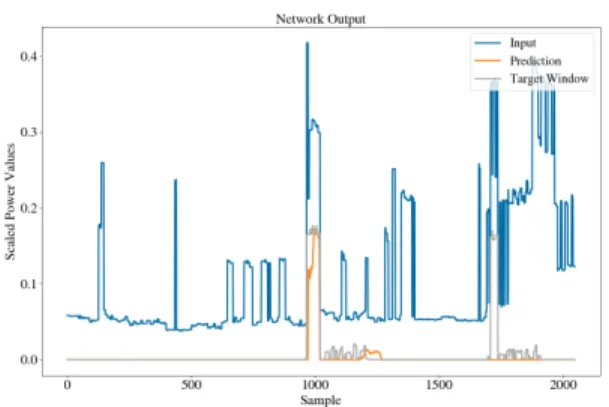
Fig. 1 shows the output of the network over a partial input window which contains two uses of the washing machine. It can be seen that the network correctly identifies the first Washing Machine operation (starting roughly at sample 100 and ending at 300). However, the second run of the washing machine (roughly between samples 800 and 10000) was not picked up by the network. Taking snapshots of the network layers and outputs at vari-ous points enables us to better understand good training vs. bad training and better helps understand the differences seen between epochs. Figs. 2 (left) and 3 (left) show the activations of the first convolutional layer (conv1d) at the encoder and the third decoder

(3)

Figure 1: Network prediction. The input is the aggregate sig-nal. The target is the washing machine signal measured us-ing appliance-level monitor, and the prediction is the output of the network.

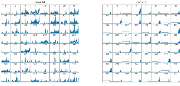
layer (conv1d_transpose_3) of the network which contain 512 and 128 filters, respectively. Note that the encoding layers are used for feature representation - to learn and extract discriminative features, while the decoding layers reconstruct the signal, hence the outputs of the latter are more ‘signal looking’. We present 64 filters in both cases to improve visibility of the figure.

We can see in the first encoder layer that filters 178 & 257 have extracted the two edges that correspond to two washing machine usages. Most other filters either missed the second usage or picked up many other appliances between the two washing machine us-ages. Some filters appear to have little activation or none at all. Assuming equal importance of each feature (i.e., each filter out-put), it becomes obvious that the second usage might be missed as features that represent this usage are not discriminative enough.

Indeed, this is propagated to the decoder side (Fig. 3 (left)), where, despite a significant amount of noise, it is obvious that most filters have a significant peak corresponding to the location of the first usage of the target appliance. Some filter outputs do have a response to the second appliance run, but usually hidden in the noise or smaller than the first peak. Consequently, after combining the filter outputs in the output layer, the second usage will be missed.

The two plots on the right in both figures (Figs. 2 & 3) show activations when the first washing machine usage is masked (that is, it is removed). At the encoder side, one can see a clear peak for most filters’ outputs around sample 900. The earlier neurons are inactive, due to zero washing machine usages caused by masking. This is propagated to the decoder side where the reconstruction clearly shows the second peak and the flat response prior to it.

These observations indicate that the first washing machine us-age in some way caused the second one to be missed. To further investigate this issue, Fig. 4 shows the difference in activations of all of the filters between the non-masked and masked input case. The horizontal axis corresponds to the neuron number, and each colour represents one filter. Note that the first layer reduces the initial input size from 2048 samples to 1024, which means that the first masked 1500 samples correspond to the first 750 samples in

this encoder layer. Since the filter window is shifted by one sample each time, there are 1024 neurons each with a receptive field of 300 corresponding to the filter size.

It can be seen from the figure that, the first 750 neurons are inac-tive in the case of the masked input, after neuron 860 compared to the non-masked input. In this case neuron 861 is the most changed from the non-masked input and we can then identify the filters that contribute to this difference the most.

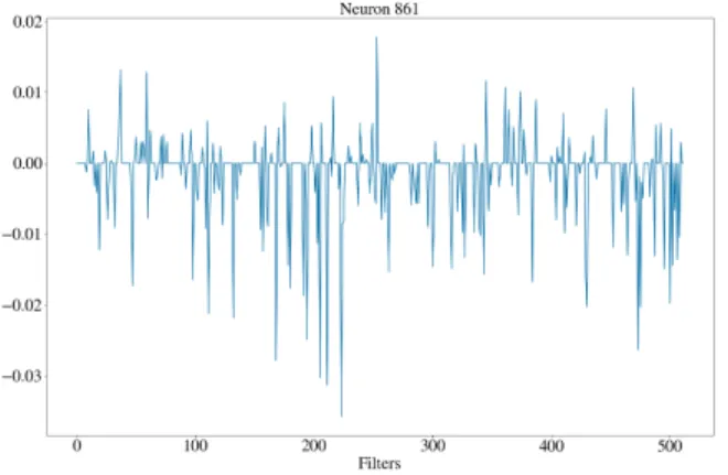
Fig. 5 shows the activation difference between non-masked and masked input for neuron 861 only, for each filter. It can be seen that filters 223, 211, 205, and 168 contribute a large amount to the successful detection of the second washing machine usage. To understand how they contribute to the network‘s overall output, we manually adjusted the filter bias in an attempt to have the non-masked input detect both the first and second activations. Understanding the interaction between the bias weights and the output is useful as if we can generate a result which detects both activations, it shows that with proper training it is possible the network to achieve this.

Once bias for the first encoder layer was adjusted in favour of the four filters mentioned previously, the output in Fig. 6 shows that both activations are detected without changing (masking) the input. The second activation is not fully realised, and the bias adjustment has meant that the original activation is slightly diminished. How-ever, the result shows how the inner workings of the network can be understood using masking. Using this knowledge it could be possible to make a network performing well, perform better with additional training on specific cases making use of masked inputs. We can explain now why, the original network correctly identified the first usage of the washing machine, and missed the second one.

4 CONCLUSION

This paper attempts to initiate the, as yet unexplored, explainabil-ity problem of NILM deep learning networks. This is critical for customers to trust the NILM feedback and NILM developers to improve training and performance. We begin by looking at a one-dimensional convolutional autoencoder network representations of NILM data trained on a specific appliance. We show human ob-servable patterns are discernible from activation plots under the assumption of prior knowledge. We study the importance of partic-ular segments of the input, by masking appliance activations. This way, we identified which neurons and filters were the most critical and by re-adjusting the bias, we succeeded to improve the outcome of the network.

ACKNOWLEDGMENTS

This work was partly supported by the European Commission under the ‘H2020-EU.3.3.1- Reducing energy consumption and carbon footprint by smart and sustainable use’ program topic, according to the Grant Agreement No. 767625. We gratefully acknowledge the support of NVIDIA Corporation with the donation of the Titan Xp GPU used for this research.

REFERENCES

[1] Alejandro Barredo Arrieta, Natalia Díaz-Rodríguez, Javier Del Ser, Adrien Ben-netot, Siham Tabik, Alberto Barbado, Salvador Garcia, Sergio Gil-Lopez, Daniel

(4)

Figure 2: Network activations for the first encoder layer recorded for the sample shown in Fig. 1. The activations on the right correspond to the case when the first washing machine usage is masked, in which case the second usage is correctly identified.

Figure 3: Network activations for the third decoder layer recorded for the sample shown in Fig. 1. The activations on the right correspond to the case when the first washing machine usage is masked, in which case the second usage is correctly identified.

Molina, Richard Benjamins, Raja Chatila, and Francisco Herrera. 2020. Explain-able ExplainExplain-able Artificial Intelligence (XAI): Concepts, taxonomies, opportuni-ties and challenges toward responsible AI.Information Fusion58 (6 2020), 82–115.

https://doi.org/10.1016/j.inffus.2019.12.012

[2] David Bau, Bolei Zhou, Aditya Khosla, Aude Oliva, and Antonio Torralba. 2017. Network dissection: Quantifying interpretability of deep visual representations. InProceedings - 30th IEEE Conference on Computer Vision and Pattern Recognition, CVPR 2017, Vol. 2017-January. Institute of Electrical and Electronics Engineers

Inc., 3319–3327. https://doi.org/10.1109/CVPR.2017.354

[3] Virginia Dignum. 2017. Responsible Artificial Intelligence: Designing AI for Human Values. ITU Journal: ICT Discoveries, Special Issue 1(2017). https:

//www.itu.int/en/journal/001/Pages/01.aspx

[4] Finale Doshi-Velez and Been Kim. 2017. Towards A Rigorous Science of Inter-pretable Machine Learning. (2 2017). http://arxiv.org/abs/1702.08608 [5] Filip Karlo Dosilovic, Mario Brcic, and Nikica Hlupic. 2018. Explainable

artifi-cial intelligence: A survey. In2018 41st International Convention on Information and Communication Technology, Electronics and Microelectronics, MIPRO 2018 - Proceedings. Institute of Electrical and Electronics Engineers Inc., 210–215.

(5)

Figure 4: Difference between non-masked and masked acti-vations for each filter in the first encoder layer. Filters are represented by different colours.

Figure 5: Difference between non-masked and masked acti-vations for neuron 861 as a function of the filter number.

Figure 6: Detection of both washing machine uses with the bias of filters 223, 211, 205 and 168 increased in the first en-coder layer

https://doi.org/10.23919/MIPRO.2018.8400040

[6] Kaiming He, Xiangyu Zhang, Shaoqing Ren, and Jian Sun. 2016. Deep residual learning for image recognition. InProceedings of the IEEE Computer Society Conference on Computer Vision and Pattern Recognition, Vol. 2016-December. IEEE

Computer Society, 770–778. https://doi.org/10.1109/CVPR.2016.90

[7] Daniel Jorde, Matthias Kahl, and Hans-Arno Jacobsen. 2019. MEED: An Un-supervised Multi-Environment Event Detector for Non-Intrusive Load Moni-toring. In2019 IEEE International Conference on Communications, Control, and Computing Technologies for Smart Grids (SmartGridComm). IEEE, 1–6. https:

//doi.org/10.1109/SmartGridComm.2019.8909729

[8] Jack Kelly and William Knottenbelt. 2015. Neural NILM. InProceedings of the 2nd ACM International Conference on Embedded Systems for Energy-Efficient Built Environments - BuildSys ’15. ACM Press, New York, New York, USA, 55–64.

https://doi.org/10.1145/2821650.2821672

[9] Christoph Klemenjak, Stephen Makonin, and Wilfried Elmenreich. 2020. To-wards comparability in non-intrusive load monitoring: On data and performance evaluation. In2020 IEEE Power and Energy Society Innovative Smart Grid Tech-nologies Conference, ISGT 2020. Institute of Electrical and Electronics Engineers Inc. https://doi.org/10.1109/ISGT45199.2020.9087706

[10] Alex Krizhevsky, Ilya Sutskever, and Geoffrey E. Hinton. 2017. ImageNet clas-sification with deep convolutional neural networks. Commun. ACM(2017). https://doi.org/10.1145/3065386

[11] Paras Lakhani and Baskaran Sundaram. 2017. Deep learning at chest radiography: Automated classification of pulmonary tuberculosis by using convolutional neural networks. Radiology284, 2 (8 2017), 574–582. https://doi.org/10.1148/radiol. 2017162326

[12] David Leslie. 2019. Understanding artificial intelligence ethics and safety.The Alan Turing Institute6 (2019), 97. https://doi.org/10.5281/zenodo.3240529

[13] Jing Liao, Georgia Elafoudi, Lina Stankovic, and Vladimir Stankovic. 2015. Non-intrusive appliance load monitoring using low-resolution smart meter data. In

2014 IEEE International Conference on Smart Grid Communications, SmartGrid-Comm 2014. https://doi.org/10.1109/SmartGridComm.2014.7007702

[14] W. James Murdoch, Chandan Singh, Karl Kumbier, Reza Abbasi-Asl, and Bin Yu. 2019. Interpretable machine learning: definitions, methods, and applications. (1 2019). https://doi.org/10.1073/pnas.1900654116

[15] David Murray, Lina Stankovic, and Vladimir Stankovic. 2017. An electrical load measurements dataset of United Kingdom households from a two-year longitudinal study.Scientific Data4 (2017). https://doi.org/10.1038/sdata.2016.122

[16] David Murray, Lina Stankovic, Vladimir Stankovic, Srdjan Lulic, and Srdjan Sladojevic. 2019. Transferability of neural network approaches for low-rate energy disaggregation. InICASSP.

[17] PrivazyPlan. [n.d.]. Recital 71 EU GDPR. https://www.privacy-regulation.eu/ en/r71.htm

[18] Udo Schlegel, Hiba Arnout, Mennatallah El-Assady, Daniela Oelke, and Daniel A. Keim. 2019. Towards a rigorous evaluation of XAI methods on time series. In

Proceedings - 2019 International Conference on Computer Vision Workshop, ICCVW 2019. https://doi.org/10.1109/ICCVW.2019.00516

[19] David Silver, Julian Schrittwieser, Karen Simonyan, Ioannis Antonoglou, Aja Huang, Arthur Guez, Thomas Hubert, Lucas Baker, Matthew Lai, Adrian Bolton, Yutian Chen, Timothy Lillicrap, Fan Hui, Laurent Sifre, George van den Driessche, Thore Graepel, and Demis Hassabis. 2017. Mastering the game of Go without human knowledge.Nature550, 7676 (10 2017), 354–359. https://doi.org/10.1038/

nature24270

[20] Christian Szegedy, Wei Liu, Yangqing Jia, Pierre Sermanet, Scott Reed, Dragomir Anguelov, Dumitru Erhan, Vincent Vanhoucke, and Andrew Rabinovich. 2015. Going deeper with convolutions. InProceedings of the IEEE Computer Society Conference on Computer Vision and Pattern Recognition. https://doi.org/10.1109/

CVPR.2015.7298594

[21] Anawat Tongta and Komkrit Chooruang. 2020. Long Short-Term Memory (LSTM) Neural Networks Applied to Energy Disaggregation. In2020 8th International Elec-trical Engineering Congress, iEECON 2020. https://doi.org/10.1109/iEECON48109.

2020.229559

[22] Laurens Van Der Maaten and Geoffrey Hinton. 2008. Visualizing data using t-SNE.Journal of Machine Learning Research(2008).

[23] T. S. Wang, T. Y. Ji, and M. S. Li. 2019. A New Approach for Supervised Power Disaggregation by Using a Denoising Autoencoder and Recurrent LSTM Network. InProceedings of the 2019 IEEE 12th International Symposium on Diagnostics for Electrical Machines, Power Electronics and Drives, SDEMPED 2019. https: //doi.org/10.1109/DEMPED.2019.8864870

[24] Jason Yosinski, Jeff Clune, Anh Nguyen, Thomas Fuchs, and Hod Lipson. 2015. Understanding Neural Networks Through Deep Visualization. (6 2015). http: //arxiv.org/abs/1506.06579

[25] Matthew D. Zeiler and Rob Fergus. 2014. Visualizing and understanding convolutional networks. InLecture Notes in Computer Science (including sub-series Lecture Notes in Artificial Intelligence and Lecture Notes in Bioinformatics).

https://doi.org/10.1007/978-3-319-10590-1{_}53

[26] Chaoyun Zhang, Mingjun Zhong, Zongzuo Wang, Nigel Goddard, and Charles Sutton. 2018. Sequence-to-point learning with neural networks for nonintrusive load monitoring.The Thirty-Second AAAI Conference on Artificial Intelligence

(6)