Towards More Scalable and Robust Machine Learning

(1)

UC Berkeley Electronic Theses and Dissertations

Title

Towards More Scalable and Robust Machine Learning Permalink https://escholarship.org/uc/item/96x8f4m0 Author Yin, Dong Publication Date 2019 Peer reviewed|Thesis/dissertation

eScholarship.org Powered by the California Digital Library University of California

(2)

by Dong Yin

A dissertation submitted in partial satisfaction of the requirements for the degree of

Doctor of Philosophy in

Engineering - Electrical Engineering and Computer Sciences in the

Graduate Division of the

University of California, Berkeley

Committee in charge:

Professor Kannan Ramchandran, Chair Professor Peter Bartlett

Professor Zuo-Jun Shen

(3)

(4)

Abstract

Towards More Scalable and Robust Machine Learning by

Dong Yin

Doctor of Philosophy in Engineering - Electrical Engineering and Computer Sciences University of California, Berkeley

Professor Kannan Ramchandran, Chair

For many data-intensive real-world applications, such as recognizing objects from images, detecting spam emails, and recommending items on retail websites, the most successful current approaches involve learning rich prediction rules from large datasets. There are many challenges in these machine learning tasks. For example, as the size of the datasets and the complexity of these prediction rules increase, there is a significant challenge in designing

scalable methods that can effectively exploit the availability of distributed computing units. As another example, in many machine learning applications, there can be data corruptions, communication errors, and even adversarial attacks during training and test. Therefore, to build reliable machine learning models, we also have to tackle the challenge ofrobustness in machine learning.

In this dissertation, we study several topics on the scalability and robustness in large-scale learning, with a focus of establishing solid theoretical foundations for these problems, and demonstrate recent progress towards the ambitious goal of building more scalable and ro-bust machine learning models. We start with the speedup saturation problem in distributed stochastic gradient descent (SGD) algorithms with large mini-batches. We introduce the no-tion of gradient diversity, a metric of the dissimilarity between concurrent gradient updates, and show its key role in the convergence and generalization performance of mini-batch SGD. We then move forward to Byzantine distributed learning, a topic that involves both scala-bility and robustness in distributed learning. In the Byzantine setting that we consider, a fraction of distributed worker machines can have arbitrary or even adversarial behavior. We design statistically and computationally efficient algorithms to defend against Byzantine fail-ures in distributed optimization with convex and non-convex objectives. Lastly, we discuss the adversarial example phenomenon. We provide theoretical analysis of the adversarially robust generalization properties of machine learning models through the lens of Radamacher complexity.

(5)

(6)

5 Rademacher Complexity for Adversarially Robust Generalization 117 5.1 Introduction . . . 117 5.2 Related Work . . . 120 5.3 Problem Setup . . . 123 5.4 Linear Classifiers . . . 124 5.5 Neural Networks . . . 128 5.6 Experiments . . . 131 5.7 Conclusions . . . 133 5.8 Proofs . . . 134 6 Conclusions 143 Bibliography 145

(8)

List of Figures

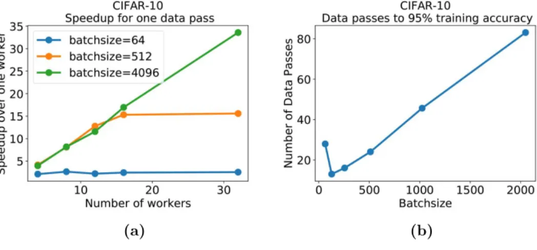
1.1 Federated Learning. The parameter server stores the model and the end users’ devices store the data. In a Federated Learning algorithm, the parameter server sends the model to the personal devices, and the devices send the local updates back to the parameter server. . . 2 2.1 (a) Speedup gains for a single data pass and various batch-sizes, for a

cuda-convnet model on CIFAR-10. (b) Number of data passes to reach 95% accuracy for a cuda-convnet model on CIFAR-10, vs batch-size. Step-sizes are tuned to maximize convergence speed. Experiments are conducted on Amazon EC2 in-stances g2.2xlarge. . . 7 2.2 Data replication. Here, 2-R, 4-R, etc represent 2-replication, 4-replication, etc,

and DC stand for DropConnect. (a) Logistic regression with two classes of CIFAR-10 (b) Cuda convolutional neural network (c) Residual network. For (a), we plot the average loss ratio during all the iterations of the algorithm, and average over 10 experiments; for (b), (c), we plot the loss ratio as a function of the number of passes over the entire dataset, and average over 3 experiments. We observe that with the larger replication factor, the gap of convergence increases. 18 2.3 Stability. (a) Normalized Euclidean distance vs number of data passes. (b)

Generalization behavior of size 512. (c) Generalization behavior of batch-size 1024. Results are averaged over 3 experiments. . . 19 3.1 Byzantine-robust distributed learning algorithm. (i) The master machine sends

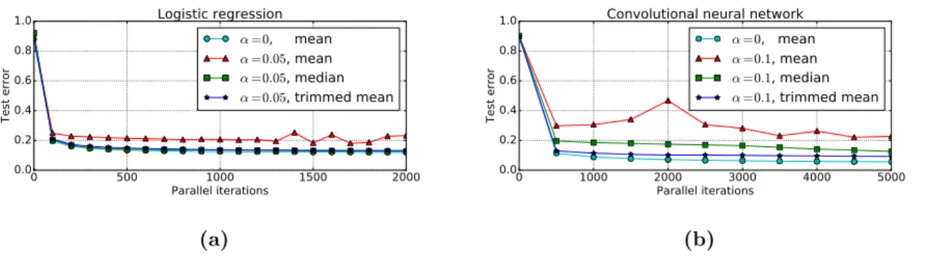
the model parameters to all the worker machines. (ii) The worker machines send either the gradient (normal machines) or an adversarial vector (Byzantine machines) to the master machine. (iii) The master machine conducts a robust aggregation. . . 46 3.2 Test error vs the number of parallel iterations. . . 56

(9)

4.1 Escaping saddle point is more difficult in the Byzantine setting. Consider a sad-dle point with e1 and e2 being the “good” and “bad” directions, respectively.

Without Byzantine machines, as long as the gradient direction has a small com-ponent on e1, the optimization algorithm can escape the saddle point. However,

in the Byzantine setting, the adversary can eliminate the component on the e1

direction and make the learner stuck at the saddle point. . . 84 5.1 Adversarially robust learning is more difficult than natural learning. . . 119 5.2 Linear classifiers. Adversarial generalization error vs `∞ perturbation and

reg-ularization coefficient λ. . . 132 5.3 Linear classifiers. Adversarial generalization error vs `∞ perturbation and

di-mension of feature space d. . . 133 5.4 Neural networks. Adversarial generalization error vs regularization coefficient λ. 134

(10)

List of Tables

2.1 Speedup Gains via DropConnect . . . 20

3.1 Comparison between the two robust distributed gradient descent algorithms. . . 52

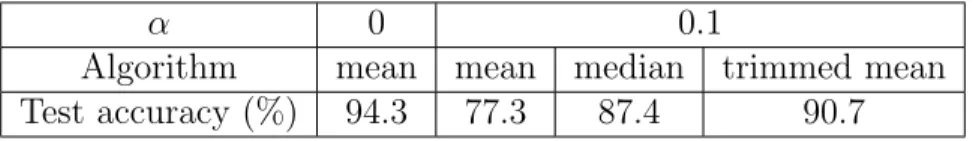
3.2 Test accuracy on the logistic regression model using gradient descent. We set m = 40, and for trimmed mean, we chooseβ = 0.05. . . 55

3.3 Test accuracy on the convolutional neural network model using gradient descent. We set m= 10, and for trimmed mean, we choose β = 0.1. . . 55

3.4 Test accuracy on the logistic regression model using one-round algorithm. We set m = 10. . . 56

4.1 Comparison with PGD, Neon+GD, and Neon2+GD. SP = saddle point. . . 86

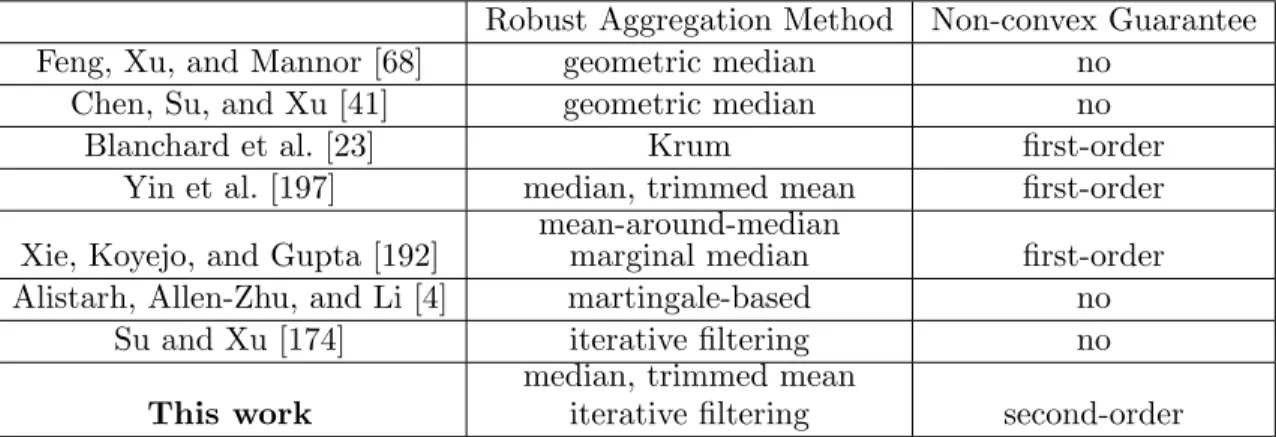
4.2 Comparison with other Byzantine-robust distributed learning algorithms. . . 86

(11)

Acknowledgments

I would like to begin with my foremost thanks to my advisor, Kannan Ramchandran. I started working with Kannan from the beginning of my PhD study, and we have closely collaborated on all my research projects at UC Berkeley. Through Kannan’s guidance, I learned all the aspects of how to do real academic research, including but not limited to identifying good problem setups, pursuing the best possible results, and writing papers that impress the readers. The most important lesson that I learned from Kannan is that as a researcher, asking a good question is perhaps more important than working out the details. In fact, Kannan is a great advisor who is really good at identifying problems that are interesting and important both theoretically and practically. Kannan also has a great vision and broad interest in many research areas. I am extremely grateful that Kannan provides me with the full freedom of choosing research directions of my own interest and encourages me to build diverse expertise in different fields.

I am also very fortunate to work with Peter Bartlett on various topics during my PhD. I started collaborations with Peter back in 2016 when I was taking his course in statisti-cal learning theory. Peter has great vision of the entire field of machine learning, including statistical learning theory, neural networks, and reinforcement learning. Peter is really knowl-edgeable about how the field of machine learning has been evolving, and has given me very useful advice from a “historical” perspective. From Peter, I learned both solid theoretical analysis techniques and approaches to finding good research directions. In particular, he always encourages me to work on challenging problems, such as proving the optimality of the results by finding matching lower bounds.

I would like to thank Max Shen, for joining my qualifying exam and dissertation com-mittees. I have heard of Max’s name in operations research when I was in my undergraduate school, and it is a pleasure to meet him at Berkeley. I sincerely appreciate his helpful sugges-tions for my dissertation. In addition, I would like to thank Laurent El Ghaoui for joining my qualifying exam committee.

During the long journey of my PhD, I was fortunate to have many amazing collaborators. I would like to give special thanks to Yudong Chen. I have known Yudong when I started my PhD at Berkeley, and at that time he was a postdoc here. During the past five years, we had many insightful discussions and nice collaborations on various topics, including learning mixtures of regressions and robust distributed learning. Yudong has helped me with many aspects of research, from technical details to the structure and writing of papers.

I would also like to thank Ramtin Pedarsani, Xiao Simon Li, and Kangwook Lee for their help with my research projects on sparse graph codes during the first two years of my PhD. I am also very grateful to Dimitris Papailiopoulos, who led me to my first research project on machine learning and distributed optimization. During the last year of my PhD, I also had many insightful discussions with Jiantao Jiao, who has shown me many smart the approaches to tackling various problems.

I would like to thank all the faculties in the BLISS research lab, for providing an open and collaborative research environment. Besides Kannan and Jiantao, the other professors

(12)

in BLISS lab are: Venkat Anantharam, Thomas Courtade, Anant Sahai, Pravin Varaiya, Martin Wainwright, and Jean Walrand. I am also grateful to all the professors of the courses that I have taken at Berkeley. I really appreciate the knowledge that I learned from the courses: they made me better prepared for my research. In a chronological order, the professors are: Thomas Courtade, Jean Walrand, Laura Waller, Benjamin Recht, Michael I. Jordan, Peter Bartlett, Martin Wainwright, Laurent El Ghaoui, Dawn Song, and Trevor Darrell. I am also thankful to Kannan Ramchandran and Shobhana Stoyanov, who were the instructors of my GSI courses, for teaching me how to teach.

During my PhD, I have done three internships, all at Google. These internships are really good opportunities for me to combine my background in academic research with more applied problems. Some of the results in my internship projects end up being published in academic conferences. I am really thankful to my internship hosts — Andr´es Mu˜noz Medina, Qifan Wang, and Justin Gilmer, for their guidance and helpful advice during the internships. In addition to the people mentioned above, I would like to thank all my other coauthors and collaborators in my ongoing projects. I won’t be able to complete my research projects without their help. Here, I list them in a chronological order: Adam S. Charles, Christopher J. Rozell, Sameer Pawar, Ashwin Pananjady, Max Lam, Sergei Vassilvitskii, Ekin D. Cubuk, Raphael Gontijo Lopes, Jonathon Shlens, Ben Poole, Avishek Ghosh, Justin Hong, Jichan Chung, Xiang Cheng, and Michael I. Jordan.

I would also like to thank my friends in the BLISS, BAIR, Simons Institute for the Theory of Computing, Google, etc. It was a pleasure to meet all of them and the insightful research discussions with some of them really opened my mind. Here, I would like to give thanks to the following people, listed in an alphabetic order: Reza Abbasi-Asl, Amirali Aghazadeh, Zeyuan Allen-Zhu, Efe Aras, Sivaraman Balakrishnan, Kush Bhatia, Niladri Chatterji, Lin Chen, Zihao Chen, Yeshwanth Cherapanamjeri, Bo Dai, Payam Delgosha, Ilias Diakonikolas, Simon S Du, Raaz Dwivedi, Giulia Fanti, Vipul Gupta, Sang Min Han, Kate Harrison, Horace He, Reinhard Heckel, Shuguang Hu, Longbo Huang, Shloak Jain, Chi Jin, Varun Jog, Rashmi K V, Swanand Kadhe, Vijay Kamble, Koulik Khamaru, Alex Kulesza, Jason Lee, Kuan-Yun Lee, Jerry Li, Shiau Hong Lim, Liu Liu, Po-Ling Loh, Phil Long, Tengyu Ma, Alan Malek, Wenlong Mou, Vidya Muthukumar, Orhan Ocal, Frank Ong, Aldo Pacchiano, Soham Phade, Yannik Pitcan, Gireeja Ranade, Ludwig Schmidt, Nihar B Shah, D. Sivakumar, Vasuki Narasimha Swamy, Hongyi Wang, Yuting Wei, Fanny Yang, Yaoqing Yang, Yun Yang, Felix Yu, Yang Yuan, Chiyuan Zhang, Yuchen Zhang, and Banghua Zhu.

I would like to give special thanks to Berkeley DeepDrive (BDD) for generously funding me for many of the semesters during my PhD. I would also like to thank many staffs in the EECS department, especially Shirley Salanio, for promptly answering my questions.

Lastly but most importantly, my foremost gratitude goes to my family. I would like to thank my wife Miao Cheng, for the sweet time that we spent together, and for her encouragement and support during the long journey of my PhD. I would also like to thank my parents and parent-in-laws for their selfless support during these years. Finally, I would like to thank our cat, Miku, for bringing so much fun to our family.

(13)

Chapter 1 Introduction

For many data-intensive real-world applications, such as recognizing objects from images, detecting spam emails, and recommending items on retail websites, the most successful current approaches involve learning rich prediction rules from large datasets. There are many challenges in these machine learning tasks. For example, as the size of the datasets and the complexity of these prediction rules increase, there is a significant challenge in designing

scalable methods that can effectively exploit the availability of distributed computing units. As another example, in many machine learning applications, there can be data corruptions, communication errors, and even adversarial attacks during training and test. Therefore, to build reliable machine learning models, we have to tackle the challenge of robustness in machine learning.

1.1 Challenges in Scalable Machine Learning

As the scale of training datasets and model parameters increases, it becomes more and more important to efficiently utilize the availability of distributed computing devices in training machine learning models. In fact, distributed optimization has become the cornerstone of many real-world machine learning applications. Many of the state-of-the-art publicly available (distributed) machine learning frameworks, such as Tensorflow [1] and MXNet [40], offer distributed implementations of popular learning algorithms. In many applications, a batch of data are distributed over multiple machines for parallel processing in order to speed up computation. In other settings, the data sources are naturally distributed, and for privacy and efficiency considerations, the data are not transmitted to a central machine. An example is the recently proposedFederated Learning paradigm [135, 108, 107], in which the data are stored and processed locally in end users’ cellphones and personal computers. We illustrate Federated Learning in Figure 1.1.

Let us consider the problem of gaining speedup using distributed computing. Ideally, the speedup gain by using parallel computing nodes should be linear, i.e., when we double the number of parallel devices, the time that we need to train a good model should be halved.

(14)

Figure 1.1: Federated Learning. The parameter server stores the model and the end users’ devices store the data. In a Federated Learning algorithm, the parameter server sends the model to the personal devices, and the devices send the local updates back to the parameter server.

However, for many machine learning algorithms, this is not true. In fact, although with more distributed computing nodes, the training algorithms are usually faster, it is often observed that, in many distributed implementation of learning algorithms, linear speedup is only possible for up to tens of computing nodes, and several studies have shown that there is a significant gap between ideal and realizable speedups when scaling out to hundreds of compute nodes [52, 153]. This commonly observed phenomenon is referred to as speedup saturation.

This phenomenon is not hard to understand when we take the communication overhead in distributed systems into account. For example, when we implement the stochastic gradient descent (SGD) algorithm in a standard system with one master machine (parameter server) and several worker machines (computing nodes), in each iteration, the master machine needs to send the model parameters to every worker machine, wait until all the worker machine finish their computation jobs and send back the results, and then update the model param-eters. In this process, the delay in communication channels and stragglers among worker machines can both be the communication overhead, and when the communication cost is comparable with the speedup gain by using more worker machines, the speedup saturation phenomenon happens.

Therefore, the key to designing communication-efficient distributed learning algorithms is reducing the communication cost. There are many approaches in the literature; how-ever, most of them can be classified into two categories: 1) reducing the total number of iterations, and 2) reducing the communication cost in each iteration. Examples of the first category are one-round algorithm [209, 206], approximate Newton method [165], large-batch

(15)

training [80], etc; and examples of the second category are asynchronous training (reducing the cost of synchronization in each iteration) [156], coded computing (reducing the effect of stragglers) [120], gradient compression (reducing the size of the messages transmitted in each iteration) [5, 189], etc.

However, we usually cannot reduce the communication cost for free, and when we apply these communication-efficient learning algorithms, there are often trade-offs between the speedup gain due to smaller communication cost and the degradation in the performance of the algorithm. For example, if we apply the one-round algorithm, in which each worker machine computes a local solution and the master machine averages them, to solve a learning problem, the final solution will suffer from an unavoidable bias since each worker machine only uses a relatively small amount of data [165]. Another example is that, in asynchronous training and gradient compression schemes, although we can gain speedup by using less accurate information about the gradients, the final solution that we get might become worse. Thus, understanding and mitigating these trade-offs are crucial to the field of distributed learning.

In this dissertation, we will focus on large-batch training—one common way to reduce the number of iterations in SGD algorithms, and study the fundamental trade-offs when using large batch sizes. We will also discuss potential approaches to mitigating these trade-offs.

1.2 Challenges in Robust Machine Learning

Robustness is another significant challenge in machine learning. In recent years, machine learning models, in particular, deep neural networks, have achieved remarkable success in many tasks on standard benchmarks. However, when we implement these models in real-world security-critical applications such as medical diagnosis and autonomous driving, it is crucial to guarantee that these models can work reliably in the presence of data corruption, distributional shift and even adversarial attacks. In practice, the robustness challenge can happen during every stage of the learning algorithm: training, test, and even both. In the following, we elaborate some training-time and test-time robustness problems.

During training, there can be noise in the features and labels [141], adversarially injected poisoning data [171], adversarial manipulation to the training algorithms and systems [23], etc. In particular, training-time robustness problem is highly related to the long-standing topic of robust statistics [89], which considers statistical estimation and inference problems under adversarially corrupted data.

In this dissertation, we discuss a training-time robustness problem in distributed learning, known as the Byzantine setting [114]. In a large-scale distributed systems, robustness and security issues have become a major concern. In particular, individual worker machines may exhibit abnormal behavior due to crashes, faulty hardware, stalled computation or unreliable communication channels. Security issues are only exacerbated in the Federated Learning setting, in which the data owners’ devices (such as mobile phones and personal computers) are used as worker machines. Such machines are often more unpredictable, and

(16)

in particular may be susceptible to malicious and coordinated attacks. Here, we note that in the Byzantine distributed learning problem, we consider a stronger attack model than in the traditional robust statistics problems, since the adversary can not only corrupt the data on some of the worker machines, they may also send malicious messages in each iteration. In this dissertation, we will design distributed optimization algorithms that are provably robust to Byzantine failures.

Robustness can also become a crucial concern during test. It has been observed that even for the models that can achieve the state-of-the-art performance in many standard benchmarks or competitions, by adversarially adding some perturbation to the input of the model (images, audio signals), these models can make wrong predictions with high confidence. These adversarial inputs are often called the adversarial examples. Typical methods of generating adversarial examples include adding small perturbations that are imperceptible to humans [177], changing surrounding areas of the main objects in images [76], and even simple rotation and translation [63]. Moreover, it has also been observed that even if the perturbations are not adversarial, some distributional shift between the training data and test data, such as common corruptions to images, can also lead to significant performance degradation [85, 157]. Both adversarial examples and distributional shift raise significant concerns about the reliablity of machine learning models in real-world applications.

Test-time robustness problems, especially the adversarial example phenomenon, are still widely open. The performance of the defense algorithms against adversarial attacks is overall not satisfactory enough [11]. In addition, currently we do not have enough theoretically principled analysis of this phenomenon. In this dissertation, we focus on the adversarially robust generalization problem, and present some rigorous analysis in this field.

1.3 Organization

In this dissertation, we study several topics on the scalability and robustness in large-scale learning, with a focus of establishing solid theoretical foundations for these problems. This dissertation is organized as follows.

In Chapter 2, we study the speedup saturation problem in distributed stochastic gradient descent (SGD) algorithms with large mini-batches. We introduce the notion of gradient diversity, a metric of the dissimilarity between concurrent gradient updates, and show its key role in the convergence and generalization performance of mini-batch SGD. We also introduce several diversity-inducing mechanisms, and provide experimental evidence indicating that these mechanisms can enable the use of larger batches without sacrificing the final accuracy, and lead to faster training in distributed learning. This chapter is based on joint work with Ashwin Pananjady, Max Lam, Dimitris Papailiopoulos, Kannan Ramchandran, and Peter Bartlett, and this work was published in Proceedings of the 21st International Conference on Artificial Intelligence and Statistics (AISTATS) in 2018 [199].

In Chapter 3, we move forward to robust distributed learning, a topic that involves both scalability and robustness in machine learning. We consider theByzantine setting, where a

(17)

fraction of distributed worker machines can have arbitrary or even adversarial behavior. We design statistically and computationally efficient algorithms for Byzantine-robust distributed learning by combining distributed gradient descent with robust estimation subroutines such as median and trimmed mean. We establish the statistical rates of the proposed algorithm with these subroutines and prove their optimality in various regimes. This chapter is based on joint work with Yudong Chen, Kannan Ramchandran, and Peter Bartlett. This work was published in Proceedings of the 35th International Conference on Machine Learning (ICML) in 2018 [197].

In Chapter 4, we continue to study Byzantine-robust distributed learning with focus on the non-convex setting. We design ByzantinePGD, an efficient and robust distributed learning algorithm that can provably escape saddle points and converge to second-order stationary points in Byzantine distributed learning. This chapter is based on joint work with Yudong Chen, Kannan Ramchandran, and Peter Bartlett. This work was published in Proceedings of the 36th International Conference on Machine Learning (ICML) in 2019 [198]. In Chapter 5, we move to the test-time adversarial robustness problem. We focus on `∞

adversarial perturbations and study the adversarially robust generalization problem through the lens of Rademacher complexity. For binary linear classifiers, we establish tight bounds for the adversarial Rademacher complexity, and show that it is never smaller than its natural counterpart, and has an unavoidable dimension dependence, unless the weight vector has bounded`1 norm. We also present extensions to multi-class linear classifiers and (non-linear) neural networks. This chapter is based on joint work with Kannan Ramchandran, and Peter Bartlett. This work was published in Proceedings of the 36th International Conference on Machine Learning (ICML) in 2019 [200].

(18)

Chapter 2 Gradient Diversity in Distributed

Learning

It has been experimentally observed that distributed implementations of mini-batch stochas-tic gradient descent (SGD) algorithms exhibit speedup saturation and decaying generaliza-tion ability beyond a particular batch-size. In this work, we present an analysis hinting that high similarity between concurrently processed gradients may be a cause of this per-formance degradation. We introduce the notion of gradient diversity that measures the dissimilarity between concurrent gradient updates, and show its key role in the convergence and generalization performance of mini-batch SGD. We also establish that heuristics simi-lar to DropConnect, Langevin dynamics, and quantization, are provably diversity-inducing mechanisms, and provide experimental evidence indicating that these mechanisms can in-deed enable the use of larger batches without sacrificing accuracy and lead to faster training in distributed learning. For example, in one of our experiments, for a convolutional neural network to reach 95% training accuracy on MNIST, using the diversity-inducing mechanism can reduce the training time by 30% in the distributed setting.

2.1 Introduction

In recent years, deploying algorithms on distributed computing units has become the de facto architectural choice for large-scale machine learning. Distributed optimization has gained significant traction with a large body of recent work establishing near-optimal speedup gains on both convex and nonconvex objectives [148, 74, 52, 201, 126, 91, 62, 37], and several state-of-the-art publicly available (distributed) machine learning frameworks, such as Tensorflow [1], MXNet [40], and Caffe2 [44], offer distributed implementations of popular learning algorithms.

Mini-batch stochastic gradient descent (SGD) is the algorithmic cornerstone for several of these distributed frameworks. During a distributed iteration of mini-batch SGD, a master node stores a global model, andP worker nodes compute gradients forBdata points, sampled

(19)

from a total of n training data (i.e., B/P samples per worker per iteration), with respect to the same global model; the parameter B is commonly referred to as the batch-size. The master, after receiving these B gradients, applies them to the model and sends the updated model back to the workers; this is the equivalent of one round of communication.

Unfortunately, near-optimal scaling for distributed variants of mini-batch SGD is only possible for up to tens of compute nodes. Several studies [52, 153] indicate that there is a significant gap between ideal and realizable speedups when scaling out to hundreds of compute nodes. This commonly observed phenomenon is referred to as speedup saturation. A key cause of speedup saturation is the communication overhead of mini-batch SGD.

Ultimately, the batch-size B controls a crucial performance trade-off between communi-cation cost and convergence speed, as observed and analyzed in several studies [178, 184, 80]. When using large batch-sizes, we observe large speedup gains per pass (i.e.,pern gradi-ent computations), as shown in Figure 2.1a, due to fewer communication rounds. However, as shown in Figure 2.1b, to achieve a desired level of accuracy for larger batches, we may need a larger number of passes over the dataset, resulting inoverallslower computation that leads to speedup saturation. Furthermore, recent work shows that large batch sizes lead to models that generalize worse [100], and efforts have been made to improve the generalization ability [86].

(a) (b)

Figure 2.1: (a) Speedup gains for a single data pass and various batch-sizes, for a cuda-convnet model on CIFAR-10. (b) Number of data passes to reach 95% accuracy for a cuda-convnet model on CIFAR-10, vs batch-size. Step-sizes are tuned to maximize convergence speed. Experiments are conducted on Amazon EC2 instances g2.2xlarge.

The key question that motivates our work is: How does the batch-size control the scala-bility and generalization performance of mini-batch SGD?

(20)

Our Contributions

We employ the notion of gradient diversity that measures the dissimilarity between concur-rent gradient updates. We show that the convergence of mini-batch SGD, on both convex and nonconvex loss functions, including the Polyak- Lojasiewicz functions [151, 128], is identical— up to constant factors—to that of serial SGD (e.g., B = 1), if the batch-size is proportional to a bound implied by gradient diversity. We also establish the worst case optimality and tightness of the bound in strongly convex functions.

Although it has been empirically observed that more diversity in the data leads to more parallelism [44], and there has been significant work on the theory of mini-batch algorithms, our results have two major novelties: 1) our batch-size bound is data-dependent, tight, and essentially identical across convex and nonconvex functions, and in some cases leads to guaranteed uniformly larger batch-sizes compared to prior work, and 2) the bound has an operational meaning, and inspired by our theory, we establish that algorithmic heuristics similar to DropConnect [183], Langevin dynamics [188], and quantization [5] are diversity-inducing mechanisms. In our experiments, we find that the proposed mechanisms can indeed enable the use of larger batch-size in distributed learning, and thus reduce training time.

Following our convergence analysis, we study the effect of batch-size on the generalization behavior of mini-batch SGD using the notion of algorithmic stability [25]. Through a similar measure of gradient diversity, we show that as long as the batch-size is below a certain threshold, then mini-batch SGD is as stable as one sample SGD that is analyzed by Hardt, Recht, and Singer [83].

2.2 Related Work

Mini-batch SGD Dekel et al. [54] analyze mini-batch SGD on non-strongly convex func-tions and propose B = O(√T) as an optimal choice for batch-size. In contrast, our work provides a data-dependent principle for the choice of batch-size, and it holds without the requirement of convexity. Even in the regime where the result in Dekel et al. [54] is valid, depending on the problem, our result may still provide better bounds on the batch-size than

O(√T) (e.g., in the sparse conflict setting shown in Section 2.4). Friedlander and Schmidt [69] propose an adaptive batch-size scheme and show that this scheme provides weak lin-ear convergence rate for strongly convex functions. De et al. [51] propose an optimization algorithm for choosing the batch-size, and weighted sampling techniques have also been developed [210, 142, 202].

Diversity and data-dependent bounds In empirical studies, it has been observed that more diversity in the data allows more parallelism [44]. As for the theoretical analysis, data-dependent thresholds for batch-size have been developed for some specific problems such as least squares [92] and SVM [178]. In particular, for least square problems, Jain et al. [92] propose a bound on batch-size similar to our measure of gradient diversity; however, as

(21)

mentioned in Section 2.1, our result holds for a wider range of problems including nonconvex setups, and can be used to motivate heuristics that result in speedup gains in distributed systems.

Other mini-batching and distributed optimization algorithms Beyond mini-batch SGD, several other mini-batching algorithms have been proposed; we survey a non-exhaustive list. Mini-batch proximal algorithms are studied by Li et al. [125], Wang, Wang, and Sre-bro [184], and Wang and SreSre-bro [186], and these algorithms require solving a regularized optimization algorithm on a sampled batch as a subroutine. Other algorithms include ac-celerated methods [46], mini-batch SDCA [164, 179], and the combination of mini-batching and variance reduction such as Acc-Prox-SVRG [147] and mS2GD [106]. Here, we emphasize that although different mini-batching algorithms can be designed for particular problems and may work better in particular regimes, especially in the convex setting, these algorithms are usually more difficult to implement in distributed learning frameworks like Tensorflow or MXNet, and can introduce additional communication costs. A few other algorithms have been recently proposed to reduce the communication cost by inducing sparsity in the gra-dients, for instance, QSGD [5] and TernGrad [189]. Other algorithms have been proposed under different distributed computation frameworks, examples include one-shot model aver-aging [212, 209], and the local storage framework [117, 165, 91].

Generalization and stability An important performance measure of a learning algorithm is its generalization ability. In their foundational work, Bousquet and Elisseeff [25] prove the equivalence between algorithmic stability and generalization. This approach is then used to establish generalization bounds for SGD by Hardt, Recht, and Singer [83]. Another approach to prove generalization bounds is to use the operator view of averaged SGD [53]. This method is extended by Jain et al. [92] to the random least-squares regression problems. Variance reduction methods are also used to develop algorithms with good generalization performance [70, 50]. In this chapter, we extend the stability approach to the mini-batch setting, and show that the generalization ability is governed by a quantity that is also function of gradient diversity.

2.3 Problem Setup

We consider the following general supervised learning setup. Suppose thatD is an unknown distribution over a sample space Z, and we have access to a sample S ={z1, . . . ,zn} of n data points, that are drawn i.i.d. from D. Our goal is to find a model w from a model space W ⊆ _Rd _{with small} _{population risk} _{with respect to a loss function} _f_, _i.e., _{we want} to minimize R(w) =_Ez∼D[f(w;z)]. Since we do not have access to the population risk, we

(22)

instead train a model whose aim is to minimize the empirical risk RS(w) := 1 n n X i=1 f(w;zi). (2.1) For any training algorithm that operates on the empirical risk, there are two important aspects to analyze: the convergence speed to a good model with small empirical risk, and the generalization gap |RS(w)−R(w)| that quantifies the performance discrepancy of the

model between the empirical and population risks. For simplicity, we use the notation fi(w) := f(w;zi), F(w) := RS(w), and define w∗ ∈ arg minw∈WF(w). In this work, we

focus on families of differentiable losses that satisfy a subset of the following for all parameters w,w0 ∈ W: Definition 2.1 (β-smooth). F(w)≤F(w0) +h∇F(w0),w−w0i+β 2kw−w 0_k2 2. Definition 2.2 (λ-strongly convex).

F(w)≥F(w0) +h∇F(w0),w−w0i+ λ

2kw−w

0_k2 2. Definition 2.3 (µ-Polyak- Lojasiewicz (PL) [151, 128]).

1 2k∇F(w)k 2 2 ≥µ(F(w)−F(w ∗ )).

Mini-batch SGD At each iteration, mini-batch SGD computes B gradients on randomly sampled data at the most current global model. At the (k+ 1)-th distributed iteration, the model is given by w(k+1)B =wkB−γ (k+1)B−1 X `=kB ∇fs`(wkB), (2.2) where each indexsi is drawn uniformly at random from [n], with replacement. Here, we use w with subscript kB to denote the model we obtain after k distributed iterations, i.e., a total of kB gradient updates. Note that we recover serial SGD when B = 1. Our results also apply to varying step-size, but for simplicity we only state our bounds with constant step-size. In related work, there is a normalization of 1/B included in the gradient step, here, without loss of generality we subsume that in the step-size γ.

We note that some of our analyses requireW to be a bounded convex subset of_Rd_{, where} the projected version of SGD can be used, by making Euclidean projections back toW,i.e.,

w(k+1)B = ΠW(wkB−γ

(k+1)B−1 X

`=kB

∇fs`(wkB)).

For simplicity, in our main text, we refer to both with/without projection algorithms as “mini-batch SGD”, but in Section 2.8 we make the distinction clear when needed.

(23)

2.4 Gradient Diversity and Convergence

In this section, we introduce our definition of gradient diversity, and state our convergence results.

Gradient Diversity

Gradient Diversity quantifies the degree to which individual gradients of the loss functions are different from each other. We note that a similar notion was introduced by Jain et al. [92] for least squares problems.

Definition 2.4 (gradient diversity). We refer to the following ratio as gradient diversity:

∆D(w) := Pn i=1k∇fi(w)k22 kPn i=1∇fi(w)k 2 2 = Pn i=1k∇fi(w)k22 Pn i=1k∇fi(w)k 2 2+ P i6=jh∇fi(w),∇fj(w)i .

Clearly, ∆D(w) is large when the inner products between the gradients taken with respect to different data points are small, and so measures diverse these gradients are. We further define a batch-size bound BD(w) for each data setS and each w∈ W:

Definition 2.5 (batch-size bound).

BD(w) :=n∆D(w).

As we see in later parts, the batch-size boundBD(w) implied by gradient diversity plays a fundamental role in the batch-size selection for mini-batch SGD.

Examples of gradient diversity We provide two examples in which we can compute a uniform lower bound for allBD(w),w∈ W. Notice that these bounds solely depend on the data setS, and are thusdata dependent.

Example 1 (generalized linear function) Suppose that any data point z consists of feature vector x ∈ _Rd _{and some label} _y _∈

R, and for sample S = {z1, . . . ,zn}, the loss function f(w;zi) can be written as a generalized linear functionf(w;zi) = `i(xTi w), where`i :R→R

is a differentiable one-dimensional function, and we do not require the convexity of`i(·). Let X= [x1 x2 · · · xn]T∈Rn×dbe the feature matrix. We have the following results for BD(w) for generalized linear functions.

Remark 2.1. For generalized linear functions, ∀ w∈ W,

BD(w)≥n min i=1,...,nkxik 2 2/σ 2 max(X).

We note that it has been shown by Tak´ac et al. [178] that the spectral norm of the data matrix is important for the batch-size choice for SVM problems, and our results have similar implication. In addition, suppose that n ≥d, and xi has i.i.d. σ-sub-Gaussian entries with

(24)

zero mean. Then there exist universal constants c1, c2, c3 > 0 such that with probability 1−c2ne−c3d, BD(w) ≥ c1d, ∀ w ∈ W. Therefore, as long as we are in the relatively high dimensional regime d= Ω(log(n)), we haveBD(w)≥Ω(d), ∀w∈ W with high probability. Example 2 (sparse conflicts) In some applications [97], the gradient of an individual loss function ∇fi(w) depends only on a small subset of all the coordinates of w (called the support), and the supports of the gradients have sparse conflict. More specifically, define a graph G = (V, E) with the vertices V representing the n data points, and (i, j) ∈ E when the supports of∇fi(w) and ∇fj(w) have non-empty overlap. Letρbe the maximum degree of all the vertices in G.

Remark 2.2. For sparse conflicts, we have BD(w)≥n/(ρ+ 1)for all w∈ W. This bound

can be large when G is sparse, i.e., when ρ is small.

Convergence Rates

Our convergence results are consequences of the following lemma, which does not require convexity of the losses, and captures the effect of mini-batching on an iterate-by-iterate basis. Here, we define M2₍_w_{) :=} 1

n Pn

i=1k∇fi(w)k22 for any w∈ W.

Lemma 2.1. LetwkB be a fixed model, and let w(k+1)B denote the model after a mini-batch

iteration with batch-size B =δBD(wkB) + 1. Then

E[kw(k+1)B−w∗k22 |wkB]≤kwkB−w∗k22−2Bγh∇F(wkB),wkB−w∗i + (1 +δ)Bγ2M2(wkB),

where equality holds when there are no projections.

As one can see, for a single iteration, in expectation, the model trained by serial SGD (B = 1), closes the distance to the optimal by exactly

2γh∇F(wkB),wkB−w∗i −γ2M2(wkB).

Our bound says that using the same step-size1 as SGD (without normalizing with a factor of B), mini-batch will close that distance to the optimal (or any critical point w∗) by ap-proximately B times more, if B =O(BD(wkB)). This matches the best that we could have hoped for: mini-batch SGD with batch-sizeB should beB times faster per iteration than a single iteration of serial SGD.

We now provide convergence results using gradient diversity. For a mini-batch SGD algorithm, define the set WT ⊂ W as the collection of all possible model parameters that the algorithm can reach duringT /B parallel iterations, i.e.,

WT :={w∈ W : w=wkB for some instance of mini-batch SGD, k = 0,1, . . . , T /B}. 1_{In fact, our choice of step-size is consistent with many state-of-the-art distributed learning} frame-works [80], and we would like to point out that this chapter provides theoretical explanation of this choice of step-size.

(25)

Our main message can be summarized as follows:

Theorem 2.1(informal convergence result). LetB ≤δBD(w)+1, ∀w∈ WT. If serial SGD

achieves an -suboptimal2 _{solution after} _T _{gradient updates, then using the same step-size}

as serial SGD, mini-batch SGD with batch-size B can achieve a (1 +δ₂)-suboptimal solution after the same number of gradient updates (i.e., T /B iterations).

Therefore, our result implies that, as long as the batch-size does not exceed the funda-mental bound implied by gradient diversity, using thesame step-size as the serial algorithm, mini-batch SGD does not suffer from convergence speed saturation.

We provide the precise statements of the results as follows. Define F∗ = minw∈WF(w),

D0 =kw0−w∗k22. In all the following results, we assume that B ≤δBD(w) + 1, ∀w∈ WT, and M2₍_w₎ _≤_M2_, _∀ _w _{∈ W}

T. The step-sizes in the following results are known to be the order-optimal choices for serial SGD with constant step-size [24, 75, 98]. We start with more general function classes, i.e.,nonconvex smooth functions and PL functions.

Theorem 2.2 (smooth functions). Suppose that F(w) is β-smooth, W =_Rd, and use step-size γ = _βM2. Then, after T ≥

2 2M2β(F(w0)−F∗) gradient updates, min k=0,...,T /B−1E[k∇F(wkB)k 2 2]≤(1 + δ 2).

Theorem 2.3 (PL functions). Suppose that F(w) is β-smooth, µ-PL, W = _Rd, and use step-size γ = _M2µ2_β, and batch-size B ≤

1 2γµ. Then, after T ≥ M2_β 4µ2 log( 2(F(w0)−F∗₎ ) gradient updates, we have _E[F(wT)−F∗]≤(1 + δ₂).

For convex loss functions, we emphasize that, there have been a lot of studies that establish similar rates, without explicitly using our notion of gradient diversity [69, 92, 178]. We present the results for completeness, and also note that via gradient diversity, we provide a general form of convergence rates that is essentially identical across convex and nonconvex objectives.

Theorem 2.4 (convex functions). Suppose that F(w) is convex, and use step-size γ = _M2. Then, after T ≥ M2_D

0

2 gradient updates, we have E[F(

B T PBT−1 k=0 wkB)−F ∗_]_≤_{(1 +} δ 2). Theorem 2.5 (strongly convex functions). Suppose that F(w)isλ-strongly convex, and use step-size γ = _Mλ2 and batch-size B ≤

1 2λγ. Then, after T ≥ M2 2λ2log( 2D0 ) gradient updates, we have _E[kwT −w∗k2 2]≤(1 + 2δ).

(26)

Worst-case Optimality

Here, we establish that the above bound on the batch-size is worst-case optimal. The fol-lowing theorem demonstrates this for a convex problem with varying agnostic batch-sizes3 Bk. Essentially, if we violate the batch bound prescribed above by a factor of δ, then the quality of our model will be penalized by a factor of δ, in terms of accuracy.

Theorem 2.6. Consider a mini-batch SGD algorithm with K iterations and varying batch-sizes B1, B2, . . . , BK, and letNk =Pk_i₌₁Bi. Then, there exists a λ-strongly convex function F(w) = _n1Pn

i=1fi(w) with bounded parameter space W, such that, if Bk ≤ 1

2λγ and Bk ≥ δ_E[BD(wNk−1)] + 1 ∀ k = 1, . . . , K (where the expectation is taken over the randomness of the mini-batch SGD algorithm), and the total number of gradient updates T =NK ≥ _λγc for

some universal constant c > 0, we have: _E[kwT −w∗k22] ≥ c

0_{(1 +}_δ)γM2

λ , where c

0 _> ₀ _is

another universal constant. More concretely, when running mini-batch SGD with step-size

γ = _Mλ2 and at least O(

M2

λ2) gradient updates, we have E[kwT −w

∗_k2

2]≥c0(1 +δ).

Although the above bound is only for strongly convex functions, it reveals that there exist regimes beyond which scaling the batch-size beyond our fundamental bound can lead to only worse performance in terms of the accuracy for a given iteration, or the number of iterations needed for a specific accuracy.

Diversity-inducing Mechanisms

In recent years, several algorithmic heuristics, such as DropConnect [183], stochastic gradi-ent Langevin dynamics (SGLD) [188], and quantization [5], have been shown to be useful for improving large scale optimization in various aspects. For example, they may help im-prove generalization or escape saddle points [71]. In this section, we demonstrate a different aspect of these heuristics. We show that gradient diversity can increase when applying these techniques independently to the data points in a batch, rendering mini-batch SGD more amenable to distributed speedup gains.

We note that these mechanisms have two opposing effects: on one hand, as we show in the sequel they allow the use of larger batch-sizes, and thus can reduce communication cost by reducing the number of iterations; on the other hand, these methods usually introduce additional variance to the stochastic gradients, and may require more iteration to achieve a particular accuracy. Consequently, there is a communication-computation trade-off inherent to these mechanisms. By carefully exploiting this trade-off, our goal would be to see a gain in the overall run time. In Section 2.6, we provide experimental evidence to show that this run time gain can indeed be observed in real distributed systems.

We use abbreviation DIM for any diversity-inducing mechanism. When data point i is sampled, instead of making gradient update ∇fi(w), the algorithm updates with a random 3_{Here, by saying that the batch-sizes are}_agnostic_{, we emphasize the fact that the batch-sizes are constants} that are picked up without looking at the progress of the algorithm.

(27)

surrogate vectorgDIM_i (w) by introducing some additional randomness, which is acquired i.i.d. across data points and iterations.

We can thus define the corresponding gradient diversity and batch-size bounds ∆DIM_D (w) := Pn i=1Ekg DIM i (w)k22 EkPni=1g DIM i (w)k22 , B_DDIM(w) :=n∆DIM_D (w),

where the expectation is taken over the randomness of the mechanism. In the following parts, we first demonstrate various diversity-inducing mechanisms, and then compareBDIM

D (w) with BD(w).

DropConnect We interpret DropConnect as updating a randomly chosen subset of all the coordinates of the model parameter vector4. LetD1, . . . ,Dn be i.i.d. diagonal matrices with diagonal entries being i.i.d. Bernoulli random variables, and each diagonal entry is 0 with drop probability p ∈ (0,1). When data point zi is chosen, we make DropConnect update gdrop_i (w) =Di∇fi(w).

Stochastic gradient Langevin dynamics (SGLD) SGLD takes the gradient updates: gsgld_i (w) = ∇fi(w) + ξi where ξi, i = 1, . . . , n, are independent isotropic Gaussian noise

N(0, σ2I).

Quantized gradients DefineQ(v) as the quantized version of a vector v. More precisely, [Q(v)]` =kvk2sgn(v`)η`(v), where η`(v)’s are independent Bernoulli random variables with

P{η` = 1}=|v`|/kvk2. We let g quant

i (w) =Q(∇fi(w)).

We can show that these mechanisms increases gradient diversity, as long asBD(w) is not already large. Formally, we have the following result.

Theorem 2.7. For any w∈ W such that BD(w)≤n, we have BDDIM(w)≥ BD(w), where DIM ∈ {drop, sgld, quant}.

2.5 Differential Gradient Diversity and Stability

In this section, we turn to another important property of mini-batch SGD algorithm, i.e.,

the generalization ability.

4_{We note that our notion of DropConnect is slightly different from the original paper [183], but is of} similar spirit.

(28)

Stability and Generalization

Recall that in supervised learning, our goal is to learn a parametric model with small popula-tion risk R(w) :=_Ez∼D[f(w;z)]. In order to do so, we use empirical risk minimization, and

hope to obtain a model that has both small empirical risk and small population risk to avoid overfitting. Formally, letAbe a possibly randomized algorithm which maps the training data to the parameter space asw=A(S). In this chapter, we use the model parameter obtained in the final iteration as the output of the mini-batch SGD algorithm,i.e.,A(S) =wT. We define the expected generalization error of the algorithm asgen(A) := ES,A[RS(A(S))−R(A(S))].

Bousquet and Elisseeff [25] show the equivalence between the generalization error and algorithmic stability. The basic idea of proving generalization bounds using stability is to bound the distance between the model parameters obtained by running an algorithm on two datasets that only differ on one data point. This framework is used by Hardt, Recht, and Singer [83] to show stability guarantees for serial SGD algorithm for Lipschitz and smooth loss functions. Roughly speaking, they show upper bounds γ on the step-size below which serial SGD is stable. This yields, as a corollary, that mini-batch SGD is stable provided the step-size is upper bounded by γ/B. We remind the reader that since we absorb the 1/B factor in the step-size, the only step-size for which the analysis by Hardt, Recht, and Singer [83] would imply stability for SGD is 1/B less than what we suggest in the convergence results. In the following parts of this section, we show that the mini-batch algorithm with a similar step-size to SGD is indeed stable, provided thedifferential gradient diversity is large enough.

Differential Gradient Diversity

The stability of mini-batch SGD is governed by thedifferential gradient diversity, defined as follows.

Definition 2.6 (differential gradient diversity and batch-size bound). For any w,w0 ∈ W,

w6=w0, the differential gradient diversity and batch-size bound is given by

∆D(w,w0) := Pn i=1k∇fi(w)− ∇fi(w 0₎_k2 2 kPn i=1∇fi(w)− ∇fi(w0)k22 , BD(w,w0) := n∆D(w,w0).

Although it is a distinct measure, differential gradient diversity shares similar properties with gradient diversity. For example, the lower bounds for BD(w) in examples 1 and 2 in Section 2.4 also hold for BD(w,w0), and two mechanisms, DropConnect and SGLD also induce differential gradient diversity, as we note Section 2.8.

(29)

Stability of Mini-batch SGD

We analyze the stability (generalization) of mini-batch SGD via differential gradient diversity. We assume that, for each z ∈ Z, the loss function f(w;z) is convex, L-Lipschitz and β-smooth in W. We choose not to discuss the generalization error for nonconvex functions, since this may require a significantly small step-size [83].

Our result is stated informally in Theorem 2.8, and holds for both convex and strongly convex functions. Here, γ is the step-size upper bound required to guarantee stability of serial SGD, and differently from the convergence results, we treat BD(w,w0) as a random variable defined by the sample S.

Theorem 2.8 (informal stability result). Suppose that, with high probability, the batch-size

B _. BD(w,w0) for all w,w0 ∈ W, w 6= w0. Then, after the same number of gradient

updates, the generalization errors of mini-batch SGD and serial SGD satisfy

gen(minibatch SGD).gen(serial SGD),

and such a guarantee holds for any step-size γ _.γ.

Therefore, our main message is that, if with high probability, batch-sizeB is smaller than BD(w,w0) for all w,w0, mini-batch SGD and serial SGD can be both stable in roughly the

same range of step-sizes, and the generalization error of mini-batch SGD and serial SGD are roughly thesame. We now provide the precise statements. In the following, we denote by₁ the indicator function.

Theorem 2.9 (generalization error of convex functions). Suppose that for any z ∈ Z,

f(w;z) is convex, L-Lipschitz and β-smooth in W. For a fixed step size γ >0, let

η=_P inf w6=w0BD(w,w 0 )< ₂ B−1 γβ −1− 1 n−11B>1 ,

where the probability is over the randomness of S. Then the generalization error of mini-batch SGD satisfies gen ≤2γL2T_n(1−η) + 2γL2T η.

It is shown by Hardt, Recht, and Singer [83] that gen(serial SGD)≤ 2γL2T_n, for convex functions, when γ ≤ 2

β. Notice that in our result, when B = 1, we get η = 0, and thus recover the generalization bound for serial SGD. Further, suppose one can find B such that infw6=w0B_D(w,w0) ≥ B with high probability. Then by choosing B ≤ 1 +δB, and γ ≤

2

β(1+δ+_n₋₁1 ), we obtain similar generalization error as the serial algorithm without significant change in the step-size range. For strongly convex functions, we have:

Theorem 2.10 (generalization error of strongly convex functions). Suppose that for any

z∈ Z, f(w;z) is L-Lipschitz, β-smooth, and λ-strongly convex in W, and B ≤ 1

2γλ. For a

fixed step size γ >0, let

η =_P inf w6=w0BD(w,w 0 )< ₂ B−1 γ(β+λ)−1− 1 n−11B>1 ,

(30)

where the probability is over the randomness of S. Then the generalization error of mini-batch SGD satisfies gen ≤ 4L

2

λn(1−η) + 2γL 2_{T η}_.

Again, as shown by Hardt, Recht, and Singer [83], we have gen(serial SGD) ≤ 4L

2

λn for strongly convex functions, when γ ≤ 2

β+λ. Thus, our remarks for the convex case above also carry over here. We also mention that while in general, the probability parameter η may appear to weaken the bound, there are practical functions for which η has rate decaying in n. For example, for generalized linear functions, we can show that when the feature vectors have i.i.d. sub-Gaussian entries, choosing B _. d yields η _. ne−d, which has polynomial decay in n whend = Ω(log(n)). For details, see Section 2.8.

2.6 Experiments

(a) (b) (c)

Figure 2.2: Data replication. Here, 2-R, 4-R, etc represent 2-replication, 4-replication, etc, and DC stand for DropConnect. (a) Logistic regression with two classes of CIFAR-10 (b) Cuda convolutional neural network (c) Residual network. For (a), we plot the average loss ratio during all the iterations of the algorithm, and average over 10 experiments; for (b), (c), we plot the loss ratio as a function of the number of passes over the entire dataset, and average over 3 experiments. We observe that with the larger replication factor, the gap of convergence increases.

We conduct experiments to justify our theoretical results. Our neural network experi-ments are all implemented in Tensorflow and run on Amazon EC2 instances g2.2xlarge. Convergence We conduct the experiments on a logistic regression model and two deep neural networks (a cuda convolutional neural network [111] and a deep residual network [84]) with cross-entropy loss running on CIFAR-10 dataset. These results are presented in Fig-ure 2.2. We use data replication to implicitly construct datasets with different gradient diversity. By replication with a factor r (or r-replication), we mean picking a random 1/r fraction of the data and replicating it r times. Across all configurations of batch-sizes, we tune our (constant) step-size to maximize convergence,e.g., to minimize training time. The sample size does not change by data replication, but gradient diversity conceivably gets

(31)

(a) (b) (c)

Figure 2.3: Stability. (a) Normalized Euclidean distance vs number of data passes. (b) Gener-alization behavior of batch-size 512. (c) GenerGener-alization behavior of batch-size 1024. Results are averaged over 3 experiments.

smaller while we increase r. We use the ratio of the loss function for large batch-size SGD (e.g., B = 512) to the loss for small batch-size SGD (e.g., B = 16) to measure the neg-ative effect of large batch sizes on the convergence rate. When this ratio gets larger, the algorithm with the large batch-size is converging slower. We can see from the figures that while we increaser, the large batch-size instances indeed perform worse, and the large batch instance performs the best when we have DropConnect, due to its diversity-inducing effect, as discussed in the previous sections. This experiment thus validates our theoretical findings. Stability We also conduct experiments to study the effect of large batch-size on the stabil-ity of mini-batch SGD. Our experiments essentially use the same technique as in the study for serial SGD by Hardt, Recht, and Singer [83]. Based on the CIFAR-10 dataset, we construct two training datasets which only differ in one data point, and train a cuda convolutional neural network using the same mini-batch SGD algorithm on these two datasets. For dif-ferent batch-sizes, we test the normalized Euclidean distance pkw−w0_k2

2/(kwk22+kw0k22) between the obtained model on the two datasets. As shown in Figure 2.3a, the normalized distance between the two models becomes larger when we increase the batch-size, which im-plies that we lose stability by having a larger batch-size. We also compare the generalization behavior of mini-batch SGD withB = 512 andB = 1024, as shown in Figures 2.3b and 2.3c. As we can see, for large batch sizes, the models exhibit higher variance in their generalization behavior, and our observation is in agreement with [100].

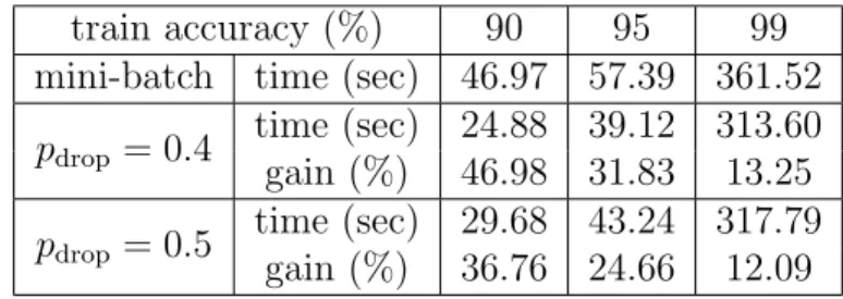
Diversity-inducing Mechanisms We finally implement diversity-inducing mechanisms in a distributed setting with 2 workers and test the speedup gains. We use a convolutional neural network on MNIST and implement the DropConnect mechanism with drop probability pdrop = 0.4,0.5. We tune the step-size γ and batch-size B for vanilla mini-batch SGD and the diversity-induced setting, and find the (γ, B) pair that gives the fastest convergence for each setting. Then, we compare the overall run time to reach 90%, 95%, and 99% training

(32)

accuracy. The results are shown in Table 2.1, where each time measurement is averaged over 5 runs. Comparing wall-clock times, we see DropConnect provides significant improvements. Indeed, the the batch-size gain afforded by DropConnect—the best batch-size for vanilla mini-batch SGD is 256, while with the diversity-inducing mechanism, it becomes 512—is able to dwarf the noise in gradient computation. Reducing communication cost thus has the biggest effect on runtime, more so than introducing additional variance in stochastic gradient computations.

Table 2.1: Speedup Gains via DropConnect

train accuracy (%) 90 95 99 mini-batch time (sec) 46.97 57.39 361.52 pdrop = 0.4 time (sec) 24.88 39.12 313.60 gain (%) 46.98 31.83 13.25 pdrop = 0.5 time (sec) 29.68 43.24 317.79 gain (%) 36.76 24.66 12.09

2.7 Conclusions

We propose the notion of gradient diversity to measure the dissimilarity between concurrent gradient updates in mini-batch SGD. We show that, for both convex and nonconvex loss functions, the convergence rate of mini-batch SGD is identical—up to constant factors—to that of serial SGD, provided that the batch-size is at most proportional to a bound implied by gradient diversity. We also develop a corresponding lower bound for the convergence rate of strongly convex objectives. Our results show that on problems with high gradient diversity, the distributed implementation of mini-batch SGD is amenable to better speedups. We also establish similar results for generalization using the notion of differential gradient diversity. Some open problems include finding more mechanisms that improve gradient diversity, and in neural network learning, studying how the network structure, such as width, depth, and activation functions, impacts gradient diversity.

2.8 Proofs

Examples of Gradient Diversity

Proof of Remark 2.1: Generalized linear models Let`0(·) be the derivative of `(·). Since we have

∇fi(w) =`0i(x T i w)xi,

(33)

by letting ai :=`0i(xiTw) and a= [a1 · · · an]T, we obtain BD(w) = nPn i=1a 2 ikxik22 kPn i=1aixik 2 2 = n Pn i=1a 2 ikxik22 kXT_a_k2 2 ≥ nmini=1,...,nkxik 2 2 Pn i=1a 2 i σ2 max(X)kak22 ≥ nmini=1,...,nkxik 2 2 σ2 max(X) ,

which completes the proof.

We made a claim after the remark about instantiating it for random design matrices. We provide the proof of that claim below.

Generalized Linear Function with Random Features We have the following two results.

Proposition 2.1. Suppose that n ≥ d, and xi has i.i.d. σ-sub-Gaussian entries with zero

mean. Then, there exist universal constants c1, c2, c3 >0, such that, with probability at least

1−c2ne−c3d, we have BD(w)≥c1d ∀ w∈ W.

Proposition 2.2. Suppose that n ≥d, and the entries of xi are i.i.d. uniformly distributed in {−1,1}. Then, there exist universal constants c4, c5, c6 >0, such that, with probability at

least 1−c5e−c6n, we have BD(w)≥c4d ∀ w∈ W.

Proof. By the concentration results of the maximum singular value of random matrices, we know that when n≥d, there exist universal constants C1, C2, C3 >0, such that

P{σmax2 (X)≤C1σ 2

n} ≥1−C2e−C3n_. _(2.3)

By the concentration results of sub-Gaussian random variables, we know that there exist universal constants C4, C5 >0 such that

P{kxik22 ≥C4σ 2

d} ≥1−e−C5d_,

and then by union bound, we have

P min i=1,...,nkxik 2 2 ≥C4σ2d ≥1−ne−C5d_. _(2.4)

Then, by combining (2.3) and (2.4) and using union bound, we obtain

P nmini=1,...,nkxik22 σ2 max(X) ≥ C4 C1 d ≥1−C2e−C3n₋_ne−C5d_,

which yields the desired result.

Proposition 2.2 can be proved using the fact that for Rademacher entries, we havekxik22 = d with probability one.

(34)

Proof of Remark 2.2: Sparse Conflict

We prove the following result for Example 2 in Section 2.4.

Proposition 2.3. Let ρ be the maximum degree of all the vertices in G. Then, we have ∀ w∈ W, BD(w)≥n/(ρ+ 1).

Proof. We adopt the convention that when (i, j)∈E, we also have (j, i)∈E. By definition, we have BD(w) = nPn i=1k∇fi(w)k22 Pn i=1k∇fi(w)k 2 2+ P i6=jh∇fi(w),∇fj(w)i = n Pn i=1k∇fi(w)k 2 2 Pn i=1k∇fi(w)k22+ P (i,j)∈Eh∇fi(w),∇fj(w)i ≥ n Pn i=1k∇fi(w)k 2 2 Pn i=1k∇fi(w)k 2 2+ P (i,j)∈E 1 2k∇fi(w)k 2 2+ 1 2k∇fj(w)k 2 2 .

Sinceρis the maximum degree of the vertexes inG, we know that for eachi∈[n], the term 1

2k∇fi(w)k 2

2 appears at most 2ρtimes in the summation P (i,j)∈E 1 2k∇fi(w)k 2 2+ 1 2k∇fj(w)k 2 2. Therefore, we obtain X (i,j)∈E 1 2k∇fi(w)k 2 2+ 1 2k∇fj(w)k 2 2 ≤ρ n X i=1 k∇fi(w)k22,

which completes the proof.

Convergence Rates

In this section, we prove our convergence results for different types of functions. To assist the demonstration of the proofs of convergence rates, for anyw∈ W, we define the following two quantities: M2(w) := 1 n n X i=1 k∇fi(w)k22 and G(w) := k∇F(w)k 2 2 =k 1 n n X i=1 ∇fi(w)k22

One can check that the batch-size bound obeysBD(w) = M2₍_w₎

(35)

Proof of Lemma 2.1 We have E[kw(k+1)B−w∗k22 |wkB] =E  kwkB−w∗ −γ (k+1)B−1 X `=kB ∇fs`(wkB)k22 |wkB   =kwkB−w∗k22−2γ (k+1)B−1 X `=kB E[hwkB−w∗,∇fs`(wkB)i |wkB] +γ2_E  k (k+1)B−1 X `=kB ∇fs`(wkB)k22 |wkB  .

Since s`’s are sampled i.i.d. uniformly from [n], we know that

E[kw(k+1)B−w∗k22 |wkB] =kwkB−w∗k22−2γBhwkB−w∗,∇F(wkB)i +γ2(BM2(wkB) +B(B−1)G(wkB)) =kwkB−w∗k22−2γBhwkB−w∗,∇F(wkB)i +γ2B 1 + B −1 BD(wkB) M2(wkB) =kwkB−w∗k22−2γBhwkB−w∗,∇F(wkB)i +γ2B(1 +δ)M2(wkB). (2.5)

We also mention here that this result becomes inequality for the projected mini-batch SGD algorithm, since Euclidean projection onto a convex set is non-expansive.

Proof of Theorem 2.2

Recall that we have the iteration w(k+1)B =wkB−γ

P(k+1)B−1

t=kB ∇fst(wkB). SinceF(w) has β-Lipschitz gradients, we have

F(w(k+1)B)≤F(wkB) +h∇F(wkB),w(k+1)B−wkBi+ β 2kw(k+1)B−wkBk 2 2. Then, we obtain * ∇F(wkB), γ (k+1)B−1 X t=kB ∇fst(wkB) + ≤F(wkB)−F(w(k+1)B) + β 2 γ (k+1)B−1 X t=kB ∇fst(wkB) 2 2 .

Now we take expectation on both sides. By iterative expectation, we know that for any t≥kB,

(36)

We also have E   (k+1)B−1 X t=kB ∇fst(wkB) 2 2  =E[BM2(wkB) +B(B −1)G(wkB)]≤B(1 +δ)M2. Consequently, γB_E[k∇F(wkB)k22]≤E[F(wkB)]−E[F(w(k+1)B)] + β 2γ 2_B_{(1 +}_δ)M2_. _(2.6) Summing up equation (2.6) for k = 0, . . . , T /B−1 yields

γB T /B−1 X k=0 E[k∇F(wkB)k22]≤F(w0)−F∗+ β 2γ 2_T_{(1 +}_δ)M2_, which simplifies to min k=0,...,T /B−1E[k∇F(wkB)k 2 2]≤ F(w0)−F∗ γT + β 2γ(1 +δ)M 2_.

We can then derive the results by replacing γ and T with the particular choices. Proof of Theorem 2.3

Substitutingw=w(k+1)Band w0 =wkB in the condition forβ-smoothness in Definition 2.1, we obtain F(w(k+1)B)≤F(wkB)−γ * ∇F(wkB), (k+1)B−1 X t=kB ∇fst(wkB) + + βγ 2 2 (k+1)B−1 X t=kB ∇fst(wkB) 2 2 .

Condition onwkB and take expectations over the choice ofst,t =kB, . . . ,(k+ 1)B−1. We obtain E[F(w(k+1)B)|wkB]≤F(wkB)−γBk∇F(wkB)k22 + βγ 2 2 BM 2₍_w kB) +B(B−1)G(wkB) . (2.7) Then, we take expectation over all the randomness of the algorithm. Using the PL condition in Definition 2.3 and the fact that B ≤1 +δBD(w) for all w∈ WT, we write

EF(w(k+1)B)−F∗

≤(1−2γµB)_E[F(wkB)−F∗] + (1 +δ)βBγ 2_M2

(37)

Then, if B ≤ 1

2γµ, we have

E[F(wT)−F∗]≤(1−2γµB)T /B(F(w0)−F∗) + (1 +δ) βγM2

4µ . Using the fact that 1−x≤e−x _{for any}_x_≥_{0, and choosing}_γ ₌ 2µ

M2_β, we obtain the desired

result.

According to Lemma 2.1, for every k = 0,1, . . . ,T_B −1, we have

E[kw(k+1)B−w∗k22 |wkB]≤ kwkB−w∗k22−2γBh∇F(wkB),wkB−w∗i+ (1 +δ)γ2BM2. Then, we take expectation over all the randomness of the algorithm. Let DkB =E[kwkB− w∗k2 2]. We have E[h∇F(wkB),wkB−w∗i]≤ 1 2γB(DkB−D(k+1)B) + (1 +δ) γ 2M 2 . (2.9) We use equation (2.9) to prove the convergence rate. We have by convexity

E  F   B T T B−1 X k=0 wkB  −F(w ∗ )  ≤E   B T T B−1 X k=0 F(wkB)−F(w∗)   = B T T B−1 X t=0 E[F(wkB)−F(w∗)] ≤ B T T B−1 X t=0 E[h∇F(wkB),wkB−w∗i] ≤ D0 2γT + (1 +δ) γM2 2 ,

where the last inequality is obtained by summing inequality (2.9) over k = 0,1, . . . ,T_B −1. Then, we can derive the results by replacing γ and T with the particular choices.

According to Lemma 2.1, we have

E[kw(k+1)B−w∗k22 |wkB]≤ kwkB−w∗k22−2γBh∇F(wkB),wkB−w∗i+(1+δ)γ2BM2(wkB). By strong convexity of F(w), we have