Multidimensional Particle Swarm Optimization for Machine Learning

Multidimensional Particle Swarm Optimization for

Machine Learning

Julkaisu 1455

•

Publication 1455

Tampereen teknillinen yliopisto. Julkaisu 1455 Tampere University of Technology. Publication 1455

Jenni Raitoharju

Multidimensional Particle Swarm Optimization for

Machine Learning

Thesis for the degree of Doctor of Science in Technology to be presented with due permission for public examination and criticism in Tietotalo Building, Auditorium TB109, at Tampere University of Technology, on the 24th _{of February 2017, at 12 noon.}

Tampereen teknillinen yliopisto - Tampere University of Technology Tampere 2017

ISBN 978-952-15-3903-9 (printed) ISBN 978-952-15-3919-0 (PDF) ISSN 1459-2045

Abstract

Particle Swarm Optimization (PSO) is a stochastic nature-inspired optimization method. It has been successfully used in several application domains since it was introduced in 1995. It has been especially successful when applied to complicated multimodal problems, where simpler optimization methods, e.g., gradient descent, are not able to find satisfactory results. Multidimensional Particle Swarm Optimization (MD-PSO) and Fractional Global Best Formation (FGBF) are extensions of the basic PSO. MD-PSO allows searching for an optimum also when the solution dimensionality is unknown. With a dedicated dimensional PSO process, MD-PSO can search for optimal solution dimensionality. An interleaved positional PSO process simultaneously searches for the optimal solution in that dimensionality. Both the basic PSO and its multidimensional extension MD-PSO are susceptible to premature convergence. FGBF is a plug-in to (MD-)PSO that can help avoid premature convergence and find desired solutions faster. This thesis focuses on applications of MD-PSO and FGBF in different machine learning tasks.

Multiswarm versions of MD-PSO and FGBF are introduced to perform dynamic opti-mization tasks. In dynamic optiopti-mization, the search space slowly changes. The locations of optima move and a former local optimum may transform into a global optimum and vice versa. We exploit multiple swarms to track different optima.

In order to apply MD-PSO for clustering tasks, two key questions need to be answered: 1) How to encode the particles to represent different data partitions? 2) How to evaluate the fitness of the particles to evaluate the quality of the solutions proposed by the particle positions? The second question is considered especially carefully in this thesis. An extensive comparison of Clustering Validity Indices (CVIs) commonly used as fitness functions in Particle Swarm Clustering (PSC) is conducted. Furthermore, a novel approach to carry out fitness evaluation, namely Fitness Evaluation with Computational Centroids (FECC) is introduced. FECC gives the same fitness to any particle positions that lead to the same data partition. Therefore, it may save some computational efforts and, above all, it can significantly improve the results obtained by using any of the best performing CVIs as the PSC fitness function.

MD-PSO can also be used to evolve different neural networks. The results of training Multilayer Perceptrons (MLPs) using the common Backpropagation (BP) algorithm and a global technique based on PSO are compared. The pros and cons of BP and (MD-)PSO in MLP training are discussed. For training Radial Basis Function Neural Networks (RBFNNs), a novel technique based on class-specific clustering of the training samples is introduced. The proposed approach is compared to the common input and input-output clustering approaches and the benefits of using the class-specific approach are experimentally demonstrated. With the class-specific approach, the training complexity is reduced, while the classification performance of the trained RBFNNs may be improved.

Collective Network of Binary Classifiers (CNBC) is an evolutionary semantic classifier consisting of several Networks of Binary Classifiers (NBCs) trained to recognize a certain semantic class. NBCs in turn consist of several Binary Classifiers (BCs), which are trained for a certain feature type. Thanks to its topology and the use of MD-PSO as its evolution technique, incremental training can be easily applied to add new training items, classes, and/or features.

In feature synthesis, the objective is to exploit ground truth information to transform the original low-level features into more discriminative ones. To learn an efficient synthesis for a dataset, only a fraction of the data needs to be labeled. The learned synthesis can then be applied on unlabeled data to improve classification or retrieval results. In this thesis, two different feature synthesis techniques are introduced. In the first one, MD-PSO is directly used to find proper arithmetic operations to be applied on the elements of the original low-level feature vectors. In the second approach, feature synthesis is carried out using one-against-all perceptrons. In the latter technique, the best results were obtained when MD-PSO was used to train the perceptrons.

In all the mentioned applications excluding MLP training, MD-PSO is used together with FGBF. Overall, MD-PSO and FGBF are indeed versatile tools in machine learning. However, computational limitations constrain their use in currently emerging machine

learning systems operating on Big Data. Therefore, in the future, it is necessary todivide

complex tasks into smaller subproblems and toconquer the large problems via solving the

subproblems where the use of MD-PSO and FGBF becomes feasible. Several applications

Preface

This study was carried out at MUVIS group at the Department of Signal Processing at Tampere University of Technology (TUT) during 2010-2016. My research was funded by TUT rector’s graduate school 2010-2014. I received additional support for conference costs from Tampere Graduate School in Information Science and Engineering (TISE) and additional financial support from Nokia Foundation and Tekniikan edistämissäätiö (TES). I was using computational resources from TUT’s Merope computing cluster and TUT grid (Techila).

I would like to express my sincere gratitude to my supervisor Prof. Moncef Gabbouj for his guidance and support. In his group, I have had the privilege to select my research topics according to my interests. Whenever I have had doubts about my own research, he has been able to return my confidence in it.

I am also thankful to Prof. Serkan Kiranyaz. He has an endless storage of innovative research ideas and it is always motivating to brainstorm these ideas with him. He has significantly contributed to every paper in this thesis. Without him, this thesis would not exist or would be at least very different, as the core content of this thesis, Multidimensional Particle Swarm Optimization, is one of his innovations.

I am grateful to my pre-examiners Prof. Salim Bouzerdoum and Prof. Nikos Nikolaidis for reviewing the thesis and giving me valuable suggestions on how to improve it. I also address special thanks to Prof. Matti Pietikäinen. I’m privileged to have him as my opponent.

I have had the pleasure to work in MUVIS group. The atmosphere in the group has been friendly and supportive. I want to thank the group as a whole and separately Dr. Iftikhar Ahmad, who has been an excellent IT support person for me and helped me to exploit computational resources, and my new office mate Dr. Alexandros Iosifidis, who has shown me an excellent example on how to be a successful postdoctoral researcher. All the way from 2007, when I started as a part-time research assistant, to the day of sending my PhD thesis to pre-examination in October 2016, my working place was in room TC413. In that room, there was always someone able to help me in any practical problems and someone willing to ponder solutions to any emerging problems, whether research-related or not. Special thanks go to my most long-term office mates, Dr. Stefan Uhlmann, Murat Birinci, Guanqun Cao, and Honglei Zhang, who have accompanied me on my way toward the goal and helped me in several ways during the years.

I thank my parents, Pirjo and Erkki, for their support and trust in my skills. During my high school years, my dad used to help me in solving the most difficult tasks in mathematics and physics. I enjoyed our joint problem solving efforts. They changed my opinion on these subjects and thrust me toward studies in a technical university.

During the last few years, my parents have always welcomed my family to their home and volunteered to wake up early with my children to provide me with the luxury of sleeping long.

My beloved husband Matti deserves enormous thanks. First of all, over the years he has concretely helped me with my research, especially in turning the huge amounts of experimental results into meaningful tables and figures. He carefully reviewed this thesis and suggested several improvements from a different viewpoint. More importantly, he has been a wonderful dad to our children. He has equally shared all the parental leaves with me. When needed, I have been able to concentrate on my research and work long hours, as I have always known that my children are in the best possible care in his hands. He has certainly improved the quality of this thesis simply by letting me sleep longer and taking more than his share of early mornings and nightly wake-ups when I was intensively writing the introductory part.

My final thanks go to my lovely children, Annikki and Ilmari. They were both born during the thesis work and they incessantly remind me that there are more important things in my life than the thesis. Sometimes they make me think that my work days are convivial and relaxing, but I always love going back home to see them again.

Tampere, December 2016 Jenni Raitoharju

Contents

Abstract i

Preface iii

Acronyms vii

Nomenclature ix

List of Publications xiii

1 Introduction 1

1.1 Thesis Objectives . . . 2

1.2 Thesis Outline . . . 2

1.3 Author’s Contribution to Publications . . . 3

2 Particle Swarm Optimization and Extensions 5 2.1 Stochastic Optimization . . . 5

2.2 PSO Algorithm . . . 6

2.3 Multi-Elitist Particle Swarm Optimization . . . 8

2.4 Multidimensional Particle Swarm Optimization . . . 9

2.5 Fractional Global Best Formation . . . 11

2.6 Multiswarm PSO . . . 13

3 Dynamic Optimization 15 3.1 Moving Peaks Benchmark . . . 15

3.2 Multiswarm FGBF and MD-PSO on (MD-)MPB . . . 17

4 Particle Swarm Clustering 21 4.1 Clustering with MEPSO . . . 22

4.2 Clustering with MD-PSO and FGBF . . . 23

4.3 Evaluation of Clustering Validity in Particle Swarm Clustering . . . 25

5 Training of Artificial Neural Networks 29 5.1 Multilayer Perceptrons . . . 30

5.2 Radial Basis Function Neural Networks . . . 34

6 Collective Network of Binary Classifiers 41 6.1 CNBC Topology . . . 42

6.2 Experimental Results . . . 43 v

7 Feature Synthesis 45 7.1 Related Work . . . 46 7.2 Evolutionary Feature Synthesis Using MD-PSO . . . 47 7.3 Feature Synthesis via One-against-all Perceptrons . . . 52

8 Conclusions 57

Bibliography 59

Errata for Publications 69

Acronyms

ACO Ant Colony Optimization

ALC-PSO Particle Swarm Optimization with an Aging Leader and Challengers

ANMRR Average Normalized Modified Retrieval Rank

ANN Artificial Neural Network

AP Average Precision

BC Binary Classifier

BP Backpropagation

CBIR Content-based Image Retrieval

CE Classification Error

CFS-EM Co-evolutionary Feature Synthesized Expectation-Maximization

CGP Co-evolutionary Genetic Programming

CNBC Collective Network of Binary Classifiers

CNN Convolutional Neural Network

CVI Clustering Validity Index

DEPSO Differential Evolution Particle Swarm Optimization

EA Evolutionary Algorithm

ECG Electrocardiogram

ECOC Error Correcting Output Code

EFS Evolutionary Feature Synthesis

EM Expectation-Maximization

EP Evolutionary Programming

ES Evolutionary Strategies

FECC Fitness Evaluation with Computational Centroids

FGBF Fractional Global Best Formation

GA Genetic Algorithm

GCPSO Guaranteed Convergence Particle Swarm Optimization

GP Genetic Programming

LFPSO Levy Flight Particle Swarm Optimization

MDA Multiple Discriminant Analysis

MD-MPB Multidimensional Moving Peaks Benchmark

MD-PSO Multidimensional Particle Swarm Optimization MEPSO Multi-Elitist Particle Swarm Optimization

MLP Multilayer Perceptron

MPB Moving Peaks Benchmark

MSE Mean Squared Error

MST Minimum Spanning Tree

NBC Network of Binary Classifiers

NCC Nearest Centroid Classifier

OED Orthogonal Experimental Design

OLPSO Orthogonal Learning Particle Swarm Optimization

PFS Perceptron Feature Synthesis

PSC Particle Swarm Clustering

PSO Particle Swarm Optimization

PSO-MAM Particle Swarm Optimization with Multiple Adaptive Methods

RBF Radial Basis Function

RBFNN Radial Basis Function Neural Network

RF Random Forest

RNN Recurrent Neural Network

SA Simulated Annealing

SAD-PSO Stochastic Approximation -driven Particle Swarm Optimization

SAR Synthetic Aperture Radar

SLP Single-layer Perceptron

SRPSO Self Regulating Particle Swarm Optimization

Nomenclature

Latin alphabet

a(·) Activation function of a neuron

A(·) Peak function in MPB

Ai ithA-type element in MD-PSO EFS encoding

bmin Minimum number of bits required for a representation

bA Artificial global best solution

bd_A Artificial global best solution in dimensionality d

bd_A,j jth element of artificial global best solution in dimensionalityd

bp Personal best solution of particle p

bdp Personal best solution of particle pin dimensionalityd

bS Global best solution

bd

S Global best solution in dimensionalityd

B Candidate group in MEPSO

B(·) Basis landscape function in MPB

Bj jth B-type element in MD-PSO EFS encoding

c Class

c1, c2 Acceleration constants in PSO

cq Center of peak qin MPB

cdq Center of peak qin dimensionalitydin MD-MPB

C Number of classes

Cj jth _cluster

d Dimensionality

dI _{Data dimensionality in input clustering}

dIO _{Data dimensionality in input-output clustering}

dmax Maximum dimensionality

dmin Minimum dimensionality

dopt Optimal dimension in MPB

dp Dimensionality of particlep

dbp Personal best dimensionality of particle p

dbS Global best dimensionality

dvp Dimensional velocity of particlep

ekp Error at neuron kfor patternp

Ep Total error for pattern p

f Feature

f(·) Fitness function for (MD)PSO

f[i] ithelement of input feature vector in EFS

fj jth feature or feature element

fj(·) Fractional fitness function for FGBF

F(·) Fitness surface function in MPB F Number of features g(·) Gaussian function hq Height of peakq in MPB hk Parameter of neuronk i, j, k Indices I Number of items

ICS _{Number of items in class-specific clustering}

II _{Number of items in input clustering}

Ij Number of items in clusterCj

K Number of clusters

KCS _{Number of clusters in class-specific clustering}

KI _{Number of clusters in input clustering}

Kmax Maximum number of clusters

l Layer index

L Number of layers

Lmax Maximum number of layers when evolving MLPs with MD-PSO

Lmin Minimum number of layers when evolving MLPs with MD-PSO

m Center location of RBF neuron

mk Center location ofkth RBF neuron

mp,j jthcluster centroid defined by position of particlep

n Neighborhood size

N Number of neurons

Ni _{Number of input neurons}

No _{Number of output neurons}

Nl

max Maximum number of neurons in layerl when evolving MLPs with MD-PSO

Nl

min Minimum number of neurons in layerl when evolving MLPs with MD-PSO

p Particle or pattern index

p[j] Index of particle having the bestjth_element

P Number of peaks

q Peak index in MPB

r, r1, r2 Random values

rbas Peak basin radius

rrep Repulsion radius

r,r1,r2 Random vectors

R Number of runs

Rmax Maximum range array for evolving MLPs with MD-PSO

Rmin Minimum range array for evolving MLPs with MD-PSO

ssw Within-cluster sum-of-squares

sq Shift vector of peakqin MPB

S Number of particles

t Iteration

tk,j jthtarget output element for classck

tkp Target output of neuronkfor pattern p

tp Target vector for patternp

T T-value in Wilcoxon Signed-Ranks test

Tp,j Activation threshold forjthcentroid defined by particlepin MEPSO

U Number of operators

xi

vmax Maximum velocity

vp Velocity of particlep

vdp Velocity of particlepin dimensionalityd

w Weight in EFS or inertia weight in PSO

wq Width of peakqin MPB

W Number of operators used to a synthesize a single feature

x Position

xd Position in dimensionality d

xp Position of particlep

xd_p Position of particlepin dimensionalityd

xd

p,j jth element of position of particlepin dimensionality d

X Search space extent

yj jth synthesized feature element

yl_k Output of neuronk in layerl

yl

kp Output of neuronk in layerl for patternp

yo_kp Output of neuronk in output layer for patternp

y Synthesized feature vector

y(j) jth synthesized feature vector

zj jth input element

z Data item or input vector

z[i] ithclosest data item

zp pthinput vector

zIO_p pthinput vector for input-output clustering

Greek alphabet

α Power parameter used in EFS fitness evaluation

β Weight for output in input-output clustering

βp Growth rate of particle pin MEPSO

γ Weight used in defining width of RBF neuron

∆h Height change severity in MPB

∆t Change interval in MPB

∆w Width change severity in MPB

η Learning rate in BP

θl

k Bias of neuronk in layerl

{θl

k} Set of biases in layerl

Θi ithoperator λ Correlation factor in MPB Λ Shift length in MPB σ Width of RBF neuron σk Width ofkthRBF neuron ωl

jk Connection weight between neuronkin layerl and itsj

th_input

{ωl

List of Publications

I Turker Ince, Serkan Kiranyaz, Jenni Pulkkinen*, Moncef Gabbouj, "Evaluation

of Global and Local Training Techniques over Feed-forward Neural Network

Ar-chitecture Spaces for Computer-aided Medical Diagnosis," Expert Systems with

Applications, vol. 37, no. 12, pp. 8450 – 8461, Dec. 2010.

II Serkan Kiranyaz, Stefan Uhlmann, Jenni Pulkkinen*, Moncef Gabbouj, Turker Ince,

"Collective Network of Evolutionary Binary Classifiers for Content-based Image

Retrieval,"IEEE Workshop on Evolving and Adaptive Intelligent Systems (EAIS

2011), pp. 147 – 154, Apr. 2011.

III Serkan Kiranyaz, Jenni Pulkkinen*, Turker Ince, Moncef Gabbouj,

"Multi-dimensional Evolutionary Feature Synthesis for Content-based Image Retrieval,"

IEEE International Conference on Image Processing (ICIP 2011), pp. 3645 – 3648,

Sep. 2011.

IV Serkan Kiranyaz, Jenni Pulkkinen*, Moncef Gabbouj, "Multi-dimensional Particle

Swarm Optimization in Dynamic Environments,"Expert Systems with Applications,

vol. 38, no. 3, pp. 2212 – 2223, Mar. 2011.

V Jenni Raitoharju, Serkan Kiranyaz, Moncef Gabbouj, "Evolutionary Feature

Syn-thesis by Multi-dimensional Particle Swarm Optimization,"European Workshop on

Visual Information Processing (EUVIP 2014), pp. 1 – 6, Dec. 2014.

VI Jenni Raitoharju, Serkan Kiranyaz, Moncef Gabbouj, "Feature Synthesis for Image

Classification and Retrieval via One-against-all Perceptrons,"Neural Computing

and Applications, pp. 1 – 15, 2016.

VII Jenni Raitoharju, Serkan Kiranyaz, Moncef Gabbouj, "Training Radial Basis

Func-tion Neural Networks for ClassificaFunc-tion via Class-Specific Clustering,"IEEE

Trans-actions on Neural Networks and Learning Systems, vol. 27, no. 12, pp. 2458 – 2471,

Dec. 2016.

VIII Jenni Raitoharju, Kaveh Samiee, Serkan Kiranyaz, Moncef Gabbouj, "Particle Swarm Clustering Fitness Evaluation with Computational Centroids," Submitted toSwarm and Evolutionary Computation, Aug. 2016.

*The former last name of Jenni Raitoharju was Pulkkinen.

1 Introduction

Over the years, numerous definitions of machine learning have been given. Some of the most quoted include

Field of study that gives computers the ability to learn without being explicitly

programmed (Arthur Samuel, 1959)

A computer program is said to learn from experience E with respect to some class of tasks T and performance measure P, if its performance at tasks in T,

as measured by P, improves with experience E. (Tom Mitchell, 1997)

Tom Mitchell defined the objectives of machine learning research as

The field of Machine Learning seeks to answer the question: How can we build computer systems that automatically improve with experience, and what are the fundamental laws that govern all learning processes?

(Tom Mitchell, 2006) Typically, machine learning tasks can be divided into supervised and unsupervised learning. In supervised learning, the desired outputs are given to the algorithm and the objective is to find a general rule that maps the inputs to the desired outputs. In unsupervised learning, the desired output is not available, but the objective is to find some internal data structures. Classification and clustering are perhaps the most obvious examples of supervised and unsupervised learning, respectively. Semi-supervised learning typically exploits a small amount of labeled data and complements the learning using a large amount of unlabeled data.

To succeed in machine learning, it is usually necessary to solve complex optimization tasks in a high-dimensional and multimodal search space. Due to local optima and a huge search space, deterministic gradient-descent-based optimization methods often cannot find proper solutions. Thus, stochastic alternatives are needed. Several stochastic optimization algorithms are inspired by natural phenomena such as genetics (e.g., Genetic Algorithm (GA) [41]) or behavior of animal populations (e.g., Ant Colony Optimization (ACO) [31], Particle Swarm Optimization (PSO) [59]). The common factor of these algorithms is that they strive for better results using an intelligent strategy while preserving some randomness in the process. This randomness can help them escape local optima and find the global optimum faster than their deterministic counterparts. The PSO algorithm mimics the interactions of an animal swarm, e.g., a bird flock or a fish school, in its search for food. The individuals are attracted toward the best feeding areas found by the

other swarm members, but simultaneously they perform their own search in a stochastic manner and may discover even better areas.

This thesis seeks to answer the questions posed by Tom Mitchell when Multidimensional Particle Swarm Optimization (MD-PSO) and Fractional Global Best Formation (FGBF) [67], which are extensions of the basic PSO, are used as tools to learn. That is, the thesis builds machine learning techniques using MD-PSO and FGBF and tries to understand the laws governing the learning processes to further improve the processes. The considered machine learning tasks include dynamic optimization, clustering, classification, image retrieval, and feature synthesis.

1.1

Thesis Objectives

The objective of this thesis was to explore the ability of MD-PSO and FGBF to solve different machine learning tasks and to modify the algorithms or applications in order to obtain a maximal benefit. More specific objectives for different applications were:

• to develop an algorithm suitable for dynamic optimization by combining MD-PSO and FGBF with multiswarms

• to improve Particle Swarm Clustering (PSC) by investigating different options for fitness evaluation

• to analyze the suitability of MD-PSO and FGBF for training neural networks and to improve training of Radial Basis Function Neural Network (RBFNN) by exploiting thedivide-and-conquer paradigm

• to use MD-PSO and FGBF to learn better features for image classification and retrieval using Collective Network of Binary Classifiers (CNBC) and feature synthesis • to develop and experimentally evaluate new methods for feature synthesis

1.2

Thesis Outline

Chapter 2 introduces the basic PSO algorithm along with its extensions. The extensions applied throughout this thesis, MD-PSO and FGBF, are introduced in sections 2.4 and 2.5. At the end of Chapter 2, multiswarm versions of PSO are discussed.

Chapter 3 concentrates on dynamic optimization. A publicly available test bench, Moving Peaks Benchmark (MPB), is introduced along with its multidimensional extension proposed in Publication IV. The chapter continues with a discussion on how to apply multiswarm FGBF and MD-PSO on (MD-)MPB. Finally, the chapter presents some experimental results from Publication IV.

PSC is the topic of Chapter 4. Different particle encoding options are explained and PSC techniques based on Multi-Elitist Particle Swarm Optimization (MEPSO) and MD-PSO with FGBF are introduced in detail. The last section discussing how to evaluate fitness in PSC is based on Publication VIII.

Chapter 5 discusses Artificial Neural Networks and how to train them with MD-PSO. Section 5.1 focuses on Multilayer Perceptrons (MLPs) and Section 5.2 on RBFNNs. For MLPs, Backpropagation (BP) and PSO training methods are compared (Publication I).

1.3. Author’s Contribution to Publications 3

For RBFNNs, a novel approach to carry out training using class-specific clustering is introduced (Publication VII).

In Chapter 6, the CNBC classifier is introduced along with its application to Content-based Image Retrieval (CBIR). Chapter 6 is based on Publication II.

Chapter 7 explains the concept of feature synthesis and its objectives. Section 7.2 describes how to use MD-PSO for Evolutionary Feature Synthesis (EFS) as originally proposed in Publication III. An improved fitness evaluation technique designed for MD-PSO-based EFS is also introduced following Publication V. Section 7.3 introduces a different feature synthesis method based on one-against-all perceptrons. This technique was originally proposed in Publication VI.

Chapter 8 concludes the introductory part of the thesis. Publications are provided at the end of the thesis.

1.3

Author’s Contribution to Publications

I The publication compares PSO and BP in training MLPs applied for solving

medical diagnosis problems. The author contributed to the implementation and the simulations reported in the paper and to the writing of the paper.

II The publication proposes using CNBC for general CBIR. Experiments on benchmark

image databases show that with CNBC a significant performance improvement is achieved over traditional retrieval techniques. The author contributed to the formulation of the problem, to the design and implementation of the experiments, and to the writing of the paper.

III The publication proposes using MD-PSO for EFS. In the proposed method,

MD-PSO is used to search for optimal arithmetic operators to transform selected elements of original low-level features into more discriminative features. The experi-ments on an image database show that the synthesized features exhibit an increased discrimination between different classes. The original idea of using MD-PSO for feature synthesis was invented by Prof. Serkan Kiranyaz. The author contributed to the design and implementation of the proposed method and to the writing of the paper.

IV The publication proposes a multiswarm version of FGBF and MD-PSO. This

version is beneficial in dynamic optimization, where the search space is slowly changing. Multiple swarms can track multiple optima and detect immediately if a former local optimum becomes the global optimum. The paper also extends MPB to a multidimensional version that allows testing in an environment where also the solution dimensionality is unknown and changing. The author implemented the multiswarm extensions of FGBF and MD-PSO as well as the multidimensional extension of MPB. She carried out the experiments, wrote several sections of the paper, and created figures 3-11.

V An improved version of feature synthesis using MD-PSO is proposed in this

publi-cation. In the improved version, a target output vector is defined for each class and MD-PSO is looking for such feature transformations that modify all the feature vectors of a class toward these target vectors. Fitness of a particle is then evaluated as the Mean Squared Error between the obtained and target feature vectors. The

computational complexity of the new fitness evaluation approach is reduced and the obtained results are better than with the approach used in Publication III. The author invented and implemented the novel approach for fitness evaluation. Prior to this publication, the improved fitness evaluation was published in another paper [82]. However, it was originally invented for this work. The author carried out the experiments and wrote the paper.

VI The publication proposes a novel technique for feature synthesis. The technique

uses parallel one-against-all perceptrons to generate new features with a higher discrimination power. This in turn leads to improved classification and retrieval results. The main merits of the proposed technique are its simplicity and faster computation compared to existing feature synthesis methods. Extensive simulations show a significant improvement in the features’ discrimination power. The author designed the work, made the required implementations, carried out the experiments, and wrote the paper.

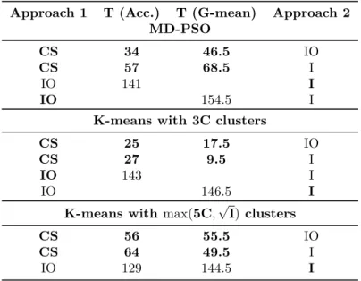
VII The publication proposes to train RBFNNs through class-specific clustering (i.e., clustering each class separately to obtain Radial Basis Function centers). This has been done in some earlier works but without considering its impact. It is shown in the paper that the class-specific approach significantly reduces the overall complexity of the clustering. Experimental comparisons against the traditional input and input-output clustering approaches are carried out using the MD-PSO, APC-III, and K-means algorithms. The results show that the class-specific approach can also lead to a significant gain in the classification performance especially when used on networks with relatively few neurons. The author designed the work, made the required implementations, carried out the experiments, and wrote the paper. VIII The publication proposes a new way to perform fitness evaluations in PSC, namely

Fitness Evaluation with Computational Centroids (FECC). An extensive compar-ison of different fitness functions in PSC is carried out using both MD-PSO and MEPSO. The proposed FECC approach is found to significantly improve clustering results. Different Clustering Validity Indices (CVIs) as fitness functions are ranked and their benefits in different situations are analyzed. The idea of FECC was born is discussions with Kaveh Samiee. The author implemented the compared CVIs, their FECC versions, and some changes to MD-PSO and FGBF. Kaveh Samiee helped checking the correctness of implemented CVIs. The author carried out the experiments and wrote the paper.

2 Particle Swarm Optimization and

Extensions

2.1

Stochastic Optimization

When randomness is involved in optimization, the process is calledstochastic optimization.

The randomness can occur in two ways: there is random noise in the fitness evaluations and/or there is randomness in the selection of the search direction. In this thesis, only the latter case is further considered. Stochastic algorithms have become popular during the last few decades in several application areas. They are mainly used in optimization problems which can be highly nonlinear, multimodal, high-dimensional, or otherwise too difficult to be solved using deterministic methods. The problems are often so challenging that it is not feasible to find the global optimum, but the randomness can help stochastic methods in avoiding some local optima and in achieving satisfactory final results. [108] In 1983, Kirkpatrick et al. proposed Simulated Annealing (SA) [71] that emulates annealing in metallurgy. In annealing, metals are first heated and then slowly cooled to improve their crystal structure and remove defects. This reduces internal stress and makes metals stronger. In SA, the search process is heated by allowing the algorithm to proceed also to solutions having worse fitness values with a certain probability. In the cooling phase, the probability of accepting worse fitness values decreases and, finally, the algorithm only accepts better solution and converges to an optimum. If the optimization problem is difficult, the final solution is still likely a local optimum. Nevertheless, annealing can help the algorithm to escape from some local optima and the final solution is usually significantly improved compared to the deterministic counterpart.

Evolutionary Algorithms (EAs) are stochastic optimization methods using techniques from biological evolution. Well-known evolutionary algorithms are Genetic Algorithm (GA) [41], Genetic Programming (GP) [8], Evolutionary Programming (EP) [36], and Evolutionary Strategies (ES) [36]. GA evolves solutions mimicking operations from genetics: mutation, crossover, and selection. Solutions are typically represented using fixed-length arrays. GP is a similar technique, but uses variable-size tree representation for the candidate solutions. Also the genetic operations used in GA and GP are slightly different. Nevertheless, the difference between the two algorithms is small [121]. Also EP and ES are similar to GA, but they emphasize different parts of natural evolution. GA emphasizes chromosomal operators, EP behavioral changes at the level of the species, and ES behavioral changes at the level of the individual [36]. Extensions of these basic algorithms have made it sometimes hard to distinguish between the methods.

Particle Swarm Optimization (PSO) belongs to the class of swarm intelligence algorithms. They are considered relatives of EAs, but, instead of natural evolution, they mimic the

behavior of animal swarms in their search for food. In addition to PSO, Ant Colony Optimization (ACO) [31] is a widely-used swarm intelligence algorithm. ACO is inspired by foraging ants. Initially, ants search randomly the surroundings of their nest. When they find some food, they deposit chemical pheromones to guide other ants toward the food.

Several comparisons of different stochastic optimization algorithms have been conducted, e.g., [5, 37, 75]. However, most comparisons are restricted to the basic versions of the stochastic optimization methods, while probably hundreds of versions of each base algorithm have been suggested. Furthermore, the comparisons usually concentrate on a very specific application area and the manually selected parameter values may significantly affect the ranking. Not surprisingly, the available comparison results are often contradictory and incomplete. Some more systematic comparison approaches have been suggested (e.g., [91]), but they have not been extensively applied. Also theoretically, it is not possible to find an optimization method that is universally successful in all kinds

of problems. Theno free lunch theorem for optimization [120] basically states that any

algorithm which is successful on certain class of optimization problems is guaranteed to perform poorly on another class. Luckily, many real world optimization problems have a similar nature and it is still possible to find algorithms performing well on several problems which are important in practice [53].

2.2

PSO Algorithm

The basic form of the PSO algorithm was introduced in [59] and later modified in [107].

In the algorithm, a swarm ofS particles explores ad-dimensional search space, where

particle positions are potential solutions to an optimization problem. Initially, each particle,p, has a random position,xp, and velocity,vp. At the beginning of each iteration, t, the new particle positions are evaluated using a problem-specific fitness function,f(xp).

Each particle remembers its personal best solution so far,bp, and the swarm as a whole

remembers the overall best solution globally achieved so far, bS. If the new particle

positions reveal better solutions,bp andbS are updated. Then the particles are moved

to a new position using the following velocity and position update functions: vp(t+ 1) =w(t)vp(t) +c1r1(t)◦(bp(t)−xp(t)) +c2r2(t)◦(bS(t)−xp(t))

xp(t+ 1) =xp(t) +vp(t+ 1), (2.1)

wherew(t) is the inertia weight,c1andc2 are the acceleration constants,r1(t) ∼ U(0,1)

andr2(t) ∼ U(0,1) are vectors of random variables uniformly distributed between

0 and 1, and ◦ denotes a Hadamard (i.e., element-wise) product of vectors. A larger

value ofw(t) favors exploration, while smaller inertia weight values favor exploitation.

Therefore, the inertia weight is often linearly decreased from a high value (e.g., 0.9) to a low value (e.g., 0.4) during iterations of a PSO run as suggested in [107]. For relatively

low-dimensional problems (e.g.,d <50), the number of particles, S, is usually set higher

than the dimensionality, S > d. However, it has been observed that the number of

iterations,R, required for convergence does not significantly depend on the number of

particles. Therefore, it is not meaningful to increase the number of particles when the problem dimensionality increases. Instead, the number of fitness evaluations (i.e., the number of particles multiplied by the number of iterations) should be increased at least linearly with respect to the problem dimensionality [20].

2.2. PSO Algorithm 7

The original PSO is not guaranteed to converge. Instead, the particle velocities have to be

controlled by setting a system coefficient, the maximum allowed velocity,vmax, to prevent

particle trajectories from swinging out of control. A lot of research has been conducted to study particle trajectories and to find such parameters that guarantee convergence. In

[24], Clerc and Kennedy showed that setting the inertia weight asw= 0.7298 and the

acceleration constants asc1=c2=c= 1.4961 results in convergent behavior. Thereafter,

these parameters have been used in most standard PSO versions. The system coefficient

vmax is no longer needed to guarantee convergence. However, it is still often used, set to

a very liberal value, in order to achieve more efficient swarm behavior [58].

Several studies have attempted to derive theoretically a parameter region guaranteeing convergence [22, 40, 57, 96, 116], but these studies have made different simplifying assumptions of the PSO process. The assumptions include, e.g., the deterministic

assumption, wherer1 andr2 have fixed values, or the stagnation assumption, wherebp

and bS have fixed values. Due to different assumptions, the studies have resulted in

different parameter regions. In [96], Poli derived the following inequality guaranteeing convergence using only the stagnation assumption:

c < 12(w

2₋₁₎

5w−7 (2.2)

In [23], this parameter region was also empirically tested to strongly correlate with the PSO convergence. However, it was noticed that setting the parameter values near the region edge leads to extremely slow convergence. Thus, the parameter values should be selected from a slightly smaller region.

It should be noted that there are no such parameters that could guarantee the basic PSO to converge to an (local) optimum [117]. The algorithm will simply reach a point of equilibrium if the parameters are properly set. Guaranteed Convergence Particle Swarm Optimization (GCPSO) [115] is a modification of the basic PSO, which has been shown to converge to an optimum. However, GCPSO only improved PSO performance on unimodal problems, especially with small swarms. On multimodal problems, GCPSO did not offer a clear advantage over the basic PSO [117]. Therefore, in general, not having a guaranteed convergence to an optimum is not a problem on more complex problems, where PSO is commonly applied.

Instead, a significant problem with the basic PSO is premature convergence to a local optimum. Even though as a stochastic search algorithm PSO can avoid some local optima, the particles typically gather close to an optimum too early. The global optimum has not been reached yet, but the algorithm loses its ability to explore new areas of the search space. Over the years, numerous modifications of the basic form of the PSO algorithm have been suggested to overcome the problem. Many modifications are based

on different swarm topologies. The basic PSO usesgbest topology, where each particle

receives information of the best solutions found by the entire swarm. In thelbesttopology,

a particle is only connected to itsnnearest neighbors. The particle neighborhoods overlap

and form a ring topology. In thelbesttopology, the information flow through the swarm is

slower and a newly found global best solution will not affect the whole swarm immediately. This has been repeatedly found to help avoid converging to a local optima [58]. However,

Engelbrecht claims in [33] thatgbest andlbest topologies have been previously compared

only on very limited datasets. In his extensive comparison, neither approach was clearly better, not even for specific problem classes.

Several PSO variants somehow modify the original bS solution to prevent premature convergence: In Multi-Elitist Particle Swarm Optimization (MEPSO) [26], which is

better introduced in Section 2.3,bS is selected among thebp based on their growth rate

βp. In Stochastic Approximation -driven Particle Swarm Optimization (SAD-PSO) [62],

stochastic approximation is used to guide thebSsolution. In Particle Swarm Optimization

with an Aging Leader and Challengers (ALC-PSO) [21], other swarm members challenge the current leader when it becomes aged. The lifespan of the leader correlates with its leading power, i.e., its ability to guide the swarm toward better solutions. In Self Regulating Particle Swarm Optimization (SRPSO) [110], a self-regulating inertia weight

is used for the bS solution. In Fractional Global Best Formation (FGBF) [67], an

artificial global best solution is created to compete withbS. FGBF is introduced in detail

in Section 2.5. It is also common to combine PSO with other learning strategies: In Levy Flight Particle Swarm Optimization (LFPSO) [43], Levy flight method is used to redistribute poorly performing particles. In SRPSO [110], the particles use self-perception to select their direction. In Orthogonal Learning Particle Swarm Optimization (OLPSO) [126], Orthogonal Experimental Design (OED) is used to develop a new orthogonal learning strategy that allows PSO particles to use their previous search experience more efficiently. In Particle Swarm Optimization with Multiple Adaptive Methods (PSO-MAM) [47, 48], a non-uniform mutation-based search method, an adaptive subgradient search method, and Cauchy mutation are combined with PSO.

Another problem besides the premature convergence is that the basic form of the PSO algorithm and also nearly all the variants operate in a fixed dimensionality. For clustering,

this means that the number of clusters should be knowna priori or, for neural network

training, that the network structure has to be fixed. Similarly, for other optimization tasks in data analysis, the optimal solution dimensionality is usually unknown. An amendment to this problem is introduced in Section 2.4.

Finally, the well-knowncurse of dimensionalityproblem affects PSO. The size of the search

space increases exponentially with respect to the problem dimensionality,d. However,

due to computational limitations, it is not possible to similarly increase the number of

fitness evaluations. As the number of iterations,R, affects the performance more than

the number of particles,S, the number of particles is kept relatively low to allow more

iterations. Therefore, for high-dimensional problems, S d. S positions in a search

space form a (S−1)-dimensional hyperplane and the attraction towardbS andbpmakes

it difficult to leave the hyperplane. Even though the randomness and the border effects enable escaping the current hyperplane, most of the exploration concentrates on the hyperplane. This increasingly deteriorates the results when the problem dimensionality

increases [20]. FGBF can decrease the effect of thecurse of dimensionality by providing

an additional mechanism to leave the current hyperplane.

In the next sections, the PSO extensions applied in this thesis are introduced in detail. MEPSO (Section 2.3) was used in Publication VIII for Particle Swarm Clustering (PSC). Multidimensional Particle Swarm Optimization (MD-PSO) (Section 2.4) and FGBF (Section 2.5) were used in Publications II-VIII for several applications. Multiswarm versions (Section 2.6) were used in Publication IV for dynamic optimization.

2.3

Multi-Elitist Particle Swarm Optimization

In MEPSO [26], each particle has a growth rateβp. If the fitness value of particlepat

2.4. Multidimensional Particle Swarm Optimization 9

the particle having the highest growth rate among the particles whose current position

has a higher fitness than the previous global best, bS(t−1). Thus, the new global best

may not have the highest fitness value, but it has improved more during the last iteration. This can help avoid premature convergence, because the global best position will vary more. The pseudocode of MEPSO, as applied in Publication VIII, is given in Listing 2.1.

MEPSO is run for Riterations.

Listing 2.1: Pseudocode of MEPSO

%Initialization 1 forp= 1 toSdo: 1.1 randomizexp(1),vp(1) 1.2 initializebp(0) =xp(1) 2 initializebS(0) =x1(1) 3 initializeβp(0) = 0 %MEPSO process 4 fort= 1 toRdo:

%Updates of growth rate and personal best solutions 4.1 forp= 1 toSdo:

4.1.1 evaluate the fitness of particle positionf(xp(t)) 4.1.2 iff(xp(t))< f(xp(t−1)) then setβp(t) =βp(t−1) + 1 4.1.3 iff(xp(t))< f(bp(t−1)) then setbp(t) =xp(t) 4.1.4 else setbp(t) =bp(t−1)

4.1.5 iff(xp(t))< f(bS(t−1)) then move particlepto a candidate groupB %Update global best

4.2 if|B|>0 sethto be index the particle with the highestβand setbS(t) =bh(t) 4.3 else setbS(t) =bS(t−1)

%Velocity and position updates 4.4 forp= 1 toSdo:

4.4.1 computevp(t+ 1) andxp(t+ 1) using Eq. (2.1)

2.4

Multidimensional Particle Swarm Optimization

MD-PSO [63, 67] is an extension of the basic PSO algorithm providing a solution to the problem of fixed solution dimensionality. MD-PSO particles perform interleaved dimen-sional and positional PSO processes. The former optimizes the solution dimendimen-sionality, while the latter aims at finding the positional optima in particles’ current dimensionalities.

For the dimensional process, each particlepknows its current dimensionality,dp,

dimen-sional velocity, dvp, and personal best dimensionality so far,dbp. The swarm as a whole

keeps track of the overall best dimensionality globally achieved so far, dbS. In the same

manner as the regular positional PSO, the dimensional PSO process uses the personal best dimensionality of each particle and the global best dimensionality to attract the particles toward better dimensional solutions.

For each dimensionality, d∈ {dmin, . . . , dmax}, particles have separate positional PSO

components. Positional PSO processes correspond to traditional PSO processes running in a given dimensionality. For the positional processes, the swarm keeps track of the

global best position so far achieved,bd

Dimensional Positional Positional 1 2 1 1 22 1 2 3 1 2 3 1 2 3 1 2 3 1 2 3 1 2 3 1 2 3 1 2 3 1 2 3 4 5 4 5 4 5 4 5 4 5 4 5 6 7 8 9 6 7 8 9 6 7 8 9

d

(t)

dv

(t)

db

(t)

MD PSO particle

bPSO particle

( 3 pt) ( 3 pt) ( 3 pt) x v b ( 2 pt) ( 2 pt) ( 2 pt) x v b ( 9 pt) ( 9 pt) ( 9 pt) x v b ( pt) ( pt) ( pt) x v b

Figure 2.1: MD-PSO particles have dimensional and positional components, while basic PSO

(bPSO) particles only have positional components. Here, the dimensional range of MD-PSO is {2, . . . ,9}and the dimensionality of the PSO solutions is fixed to 5. The current dimensionality, dp, of MD-PSO position is 2 and the personal best dimension,dbp, is 3.

xd_{p, velocity,v}d_{p, and personal best position,b}d_{p. Thus, the particles can continue their}

positional search whenever the dimensional updates move them into the particular

dimensionality d. The difference of MD-PSO particles and regular PSO particle is

illustrated in Fig. 2.1.

As with the basic PSO algorithm, a fitness score for each particlepin its current

dimen-sionality,dp, is computed at the beginning of MD-PSO iterations. After this, personal best

solutions for all particles in their current dimensionalities,bdp

p ,∀p∈ {1, . . . , S}, personal best dimensionalities for all particles, dbp,∀p∈ {1, . . . , S}, the global best solution in

each dimensionality,bd_S,∀d∈ {dmin, . . . , dmax}, and the global best dimension,dbS, are

updated, if necessary. Then particle positions and velocities are updated in their current dimensionality using (regular) positional PSO updates. The updates are the same as those given in Eq. (2.1), except now the dimensionality of the components depends on the particle’s current dimensionality, i.e., the positions and velocities in a particular

dimensionalitydhave delements.

vdp p (t+ 1) =w(t)v dp p (t) +c1r1(t)◦ bdp p (t)−x dp p (t) +c2r2(t)◦ bdp S (t)−x dp p (t) xdp p (t+ 1) =x dp p (t) +v dp p (t+ 1). (2.3)

After the positional updates, the particle’s new position,xdp

p (t+ 1), still has the same

dimensionality,dp(t). Next, the particle goes through dimensional updates, which may

move it into another dimensionality. The positional search will continue fromxdp

p (t+ 1),

if the particle is later moves back to dimensionality dp(t). Therefore, in all the other

dimensionalities, the positional PSO components for iterationt+ 1 are equal to those

for iteration t (i.e., vd_{p(t+ 1) = v}d_{p(t), x}d_{p(t+ 1) = x}d_{p(t), b}d_{p(t+ 1) = b}d_{p(t),∀d ∈}

{dmin, . . . , dmax}, d6=dp). The dimensional PSO updates closely resemble the positional

ones:

dvp(t+ 1) =bdvp(t) +c1r1(t) (dbp(t)−dp(t)) +c2r2(t) (dbS(t)−dp(t))c

2.5. Fractional Global Best Formation 11

where b· c denotes the floor operator. At the end of the MD-PSO algorithm (after R

iterations), the global best dimensionality, dbS, and the global best solution in that

dimensionality,bdbS

S , represent the optimal dimensionality and solution, respectively. The

pseudocode of MD-PSO is given in Listing 2.2 and further details of the algorithm can be found in [63].

Listing 2.2: Pseudocode of MD-PSO

%Initialization

1 forp= 1 toSdo:

1.1 randomizedp(1), dvp(1) 1.2 initializedbp(0) =dp(1) 1.3 ford=dmin todmaxdo:

1.3.1 randomizexd

p(1),vdp(1) 1.3.2 initializebd

p(0) =xdp(1) 2 initializedbS(0) =d1(1)

3 ford=dmintodmaxdo: 3.1 initializebd

S(0) =xd1(1) %MD-PSO process

4 fort= 1 toRdo:

%Updates of personal and global best solutions 4.1 ford=dmin todmaxdo:

4.1.1 setbd S(t) =bdS(t−1) 4.1.2 forp= 1 toSdo: 4.1.2.1 setbd p(t) =bdp(t−1) 4.2 forp= 1 toSdo:

4.2.1 compute the fitness of particle position,f(xdpp(t)(t)) 4.2.2 iff(xdpp(t)(t))< f(b dp(t) p (t−1)) then setb dp(t) p (t) =x dp(t) p (t) 4.2.3 iff(xdpp(t)(t))< f(b db(t−1) p (t−1)) then setdbp(t) =dp(t) 4.2.4 iff(bdpp(t)(t))< f(b dp(t) S (t)) then setb dp(t) S (t) =b dp(t) p (t) 4.3 dbS(t) = arg min d∈{dmin,...,dmax} (f(bd S(t)))

%Velocity and position updates 4.4 forp= 1 toSdo:

%Regular positional PSO updates 4.4.1 computevdpp(t)(t+ 1) andx

dp(t)

p (t+ 1) using Eq. (2.3) 4.4.2 in other dimensions thandp(t), updatevd

p(t+ 1) =vdp(t) and

xd

p(t+ 1) =xdp(t) %Dimensional PSO updates

4.4.3 computedvp(t+ 1) anddp(t+ 1) using Eq. (2.4)

2.5

Fractional Global Best Formation

The basic PSO algorithm, as well as its multidimensional extension MD-PSO, may suffer from premature convergence to a local optimum particularly in high-dimensional multimodal optimization tasks. FGBF [67] is a plug-in to the (MD-)PSO process that can efficiently address the premature convergence problem. FGBF can also decrease the

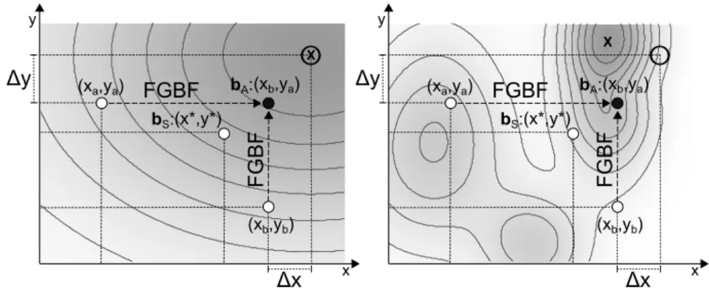
X bA: y x FGBF FGBF (xa,ya) (x*,y*) (xb,yb) (xb,ya) bS: Δx Δy X bA: y x FGBF FGBF (xa,ya) (x*,y*) (xb,yb) (xb,ya) bS: Δx Δy

Figure 2.2: FGBF used in a unimodal (left) and a multimodal (right) optimization problem.

The overall fitness surface is shown by the background color and the global optimum withx. On both sides, the fractional fitness function is a distance to referenceOand thebA solution created by FGBF turns out to be better than thebSsolution.

effect of thecurse of dimensionality by providing an additional mechanism to leave the

current hyperplane in high-dimensional problems, whereS < d. The main idea of FGBF

is to create an artificial global best solution, bA, at every iteration by combining the

best elements/dimensions of particles’ current solutions. This artificial solution then

competes withbS and the winner with a higher fitness value is then used in the update

function Eq. (2.1) or Eq. (2.3). Thejth_{element of a particle solution can be evaluated}

using a special fractional fitness function,fj(xd_{p,j). In the same manner as the ordinary}

PSO fitness function, the fractional fitness function must be designed separately for each class of optimization problems and the main challenge is to find such a function that will correlate well with the overall fitness function.

A simplified 2D example of the FGBF process and different fitness functions is shown in Fig. 2.2. On both sides, the fractional fitness score is simply a distance from a reference O(i.e.,fj(xp,1) = ∆xand fj(xp,2) = ∆y). Based on this measure, the best 1stelement

is found to be in particle b and the best 2nd _{element in particle a, and thus, the b}2

A solution is created by combining those elements. The overall fitness surface is shown by the background color. Darker color means higher fitness and the global optimum is

marked withx. On the left side, the optimization problem is unimodal, and the fractional

fitness function perfectly correlates with the overall fitness function. In such cases, the

bA solution will be always better or at least equally good as the bS solution. On the

right side, the overall fitness surface is multimodal and it usually means that it is not possible to find a fractional fitness function perfectly matching with the surface. However,

even then, thebAsolution may win thebS solution as on the right side of Fig. 2.2. If the

bA solution turns out to be worse than thebS solution,bS will be used in the updates

as usual.

When FGBF is used together with MD-PSO, a separate artificial solution,bdA, is created

for every dimensionality dwithin the dimensionality range{dmin, . . . , dmax}. In every

dimensionality, the bd_A solution competes with the bd_S solution. In most optimization

tasks, including those discussed in this thesis, it is possible to combine elements from

particle positions with different dimensionalities when creatingbdA. This is illustrated in

Fig. 2.3, where theb4_Asolution with dimensionality 4 is created by combining elements

2.6. Multiswarm PSO 13 1 2 1 1 22 1 2 3 1 2 1 2 3 1 2 3 1 2 3 1 2 3 4 5 4 5 4 5 6 7 8 9 6 7 8 9 6 7 8 9

Particlea Particleb Particlec

1 2 3 4 ( 2 a t) ( 2 a t) ( 2 a t) x v b ( 9 b t) ( 9 b t) ( 9 b t) x v b ( 3 c t) ( 3 c t) ( 3 c t) x v b ( 4 At) b 3 9 b,1(t) x 3 c,3(t) x 2 a,2(t) x 9 b,4(t) x

Figure 2.3: FGBF has created an artificial global best solution with dimensionality 4,b4A, by

combining elements from the current positions of particlea,b, andc. The dimensionalities of bA,xa,xb, andxc are all different.

elements are taken from particle b. The figure also illustrates, how only the current

solutions with the particle’s current dimensionality are considered when creatingbA. The

velocities or personal best solutions are not used. bAitself is simply a position/solution.

It does not need velocity or personal best as it is created separately at every iteration. The pseudocode of FGBF in MD-PSO is given in Listing 2.3 assuming that elements from particle positions with different dimensionalities can be combined. The pseudocode is plugged in between Steps 4.3 and 4.4 in Listing 2.2. Further details of FGBF can be found in [63].

Listing 2.3: Pseudocode of FGBF in MD-PSO

%Compute fractional fitness scores 1 forp= 1 toSdo:

1.1 forj= 1 todp(t) do: 1.1.1 computefj(xd_p,jp(t)(t))

%Find the best fractional fitness score for each elementj 2 forj= 1 todmax do:

2.1 setp[j] = arg min p∈{1,...,S}(

fj(xd p,j(t)))

%Create solutionbA in every dimension of the search space 3 ford=dmintodmaxdo:

3.1 forj= 1 toddo:

3.1.1 bd

A,j(t) =x d p[j],j(t)

%In each dimension competebA withbS 3.2 iff(bd A(t))< f(b d S(t)) thenb d S(t) =b d A(t) %UpdatedbS

4 setdbS(t) = arg min d∈{dmin,...,dmax}

(f(bd S(t)))

5 return

2.6

Multiswarm PSO

When PSO or its extension is applied, the swarm will eventually converge close to the best solution found by the swarm. In static environments, this can help fine-tune the solution

to reach the exact optimum and it can be considered a desired property if convergence is not premature. In dynamic environments, the locations and heights of the optima can vary and a former local optimum may later become the global optimum. If the whole PSO swarm is gathered around the initially global optimum, it can probably follow moderate changes in the location of this optimum. However, if another optimum becomes the global optimum, the swarm may not detect the change.

Blackwell and Branke [15] addressed this problem by introducing multiswarms. The main idea of multiswarms is that swarms can converge on separate promising optima and together they can establish a comprehensive coverage of the whole search space. The multiswarms are basically separate PSO processes. The particles are only aware of their own process. The only interaction between the swarms is a mutual repulsion preventing two swarms from converging on the same optimum. For this purpose, a repulsion radius,

rrep, is defined according to the average radius of the peak basin,rbas. IfP peaks are

evenly distributed in ad-dimensional space whose extent isX, the repulsion radius can

be defined asrrep=rbas=X/P1/d. If two swarms move withinrrepfrom each other, the

worse performing swarm is simply reinitialized. Physical repulsion is not used, because it could lead to an equilibrium where the mutual repulsion prevents both swarms from approaching an optimum. In an optimal case, the number of multiswarms coincides with the number of optima to be followed. However, in real-life problems the number of optima is usually unknown and may also vary. Therefore, Blackwell suggested also self-adapting multiswarms [12], which can be created or removed during the PSO process.

For a single swarm converging to an optimum, it is essential to maintain enough diversity to be able to follow the optimum despite small changes in its location. Early attempts to maintain required diversity include charged swarms [13] and quantum swarms [15]. In [98] and in Publication IV, we proposed using FGBF as the mechanism to ensure sufficient diversity.

2.6.1

Multiswarms with FGBF and MD-PSO

When multiswarms and FGBF are combined as originally proposed in [98], the mul-tiswarms can track different optima, while FGBF ensures that each swarm can keep tracking an optimum regardless of minor changes in its location. In Publication IV, we proposed combining multiswarms, FGBF, and MD-PSO. This allows us to perform dynamic optimization also in environments where the solution dimensionality is unknown and varying.

We use the above described repulsion radius to reinitialize swarms, if they get too close to each other. We compute the distance between two swarms as the distance of their

bS positions. To add further diversity, we reinitialize randomly the particle velocities

after each environmental change. In the multidimensional case, particle dimensions and dimensional velocities are also reinitialized.

3 Dynamic Optimization

Many real-world datasets have a dynamic nature. Data may be added or removed and data values may be updated. Solving optimization tasks in such constantly changing environments requires specialized techniques. Restarting an optimization algorithm after each system and/or environmental change would lead to a significant loss of useful information when the change is not too drastic. For example, handling video segmentation as a series of static image segmentation tasks without exploiting the similarities between consecutive frames would waste computational resources. Most dynamic optimization problems in machine learning are also multimodal and, therefore, the need of efficient optimization techniques, which are capable of adapting to the changes, is imminent. EAs designed for dynamic environments started appearing at the end of 1990s, e.g., [3, 6, 17]. Soon many PSO-based approaches were also suggested, e.g., [14, 15, 32, 55, 78]. For dynamic optimization, we proposed in Publication IV to use a combination of multiswarms and FGBF in a fixed dimension and a combination of multiswarms, FGBF, and MD-PSO when the solution dimension is unknown. These algorithms were introduced in Chapter 2. They were tested on Moving Peaks Benchmark (MPB) and its multidimensional extension proposed in Publication IV.

3.1

Moving Peaks Benchmark

MPB [18] is a configurable dynamic environment designed for testing dynamic optimization algorithms in a standard way in a multimodal environment. MPB allows the creation of different dynamic fitness surfaces consisting of a number of peaks with varying locations,

heights, and widths. The primary performance measure used is offline error, which is

the average difference between the optimum and the best solutions found since the last environmental change.

Ad-dimensional fitness surface withP peaks is expressed as

F(x, t) = max B(x), max q∈{1,...,P}(A(x, hq(t), wq(t),cq(t))) , (3.1)

whereB(x) is a time invariant basis landscape, whose utilization is optional, and Ais

a function defining the height of the qth _{peak at positionx. Each of the P peaks has}

its own dynamic parameters: heighthq(t), widthwq(t), and position of the peak center

cq(t).

Each peak parameter can be initialized randomly or set to a certain value and then after

every ∆t iterations the parameter values are changed. The change over a single peakqat