3-2018
Multivariate random parameters zero-inflated
negative binomial regression for analyzing urban
midblock crashes
Chenhui Liu
Iowa State University, [email protected] Mo Zhao
Virginia Department of Transportation
Wei Li
University of Alabama See next page for additional authors
Follow this and additional works at:https://lib.dr.iastate.edu/ccee_pubs
Part of theCivil Engineering Commons,Multivariate Analysis Commons, and the
Transportation Engineering Commons
The complete bibliographic information for this item can be found athttps://lib.dr.iastate.edu/ ccee_pubs/178. For information on how to cite this item, please visithttp://lib.dr.iastate.edu/ howtocite.html.
This Article is brought to you for free and open access by the Civil, Construction and Environmental Engineering at Iowa State University Digital Repository. It has been accepted for inclusion in Civil, Construction and Environmental Engineering Publications by an authorized administrator of Iowa State University Digital Repository. For more information, please [email protected].
for analyzing urban midblock crashes
Abstract
Urban midblock crashes are influenced mainly by traffic operation and roadway geometric features. In this paper, 10-year crash data from 1,506 directional urban midblock segments in Nebraska were analyzed using the multivariate random parameters zero-inflated negative binomial model to account for unobserved heterogeneity produced by correlations across segments, correlations across crash collision types, excessive zero crashes, and over dispersion. The multivariate random parameters zero-inflated negative binomial model was superior to many common crash frequency models in terms of both goodness of fit and prediction accuracy. Compared with the multivariate fixed parameters zero-inflated negative binomial model, the
multivariate random parameters zero-inflated negative binomial model identified fewer key influencing factors and revealed segment-specific effects of these factors on different crash types. It showed that the number of lanes, annual average daily traffic per lane, and segment length might have non-positive effects on crash frequencies. Segments with a speed limit of 45 mph had fewer crashes than did those with lower speed limits, and there were fewer crashes on the segments in Omaha than on those in Lincoln. It was also found that neither the presence of a shoulder, on-street parking, or one-way traffic, nor lane width had significant influences on crash frequencies. These findings are informative for transportation agencies to take correct and efficient measures to accommodate diverse transportation demands without reducing traffic safety. By contrast, the fixed parameters model produced results consistent with intuition, but the results were insufficient to provide actionable recommendations.
Keywords
Unobserved heterogeneity, Multivariate random parameters zero-inflated negative binomial model, Crash frequency, Urban midblock segments, Bayesian
Disciplines
Civil and Environmental Engineering | Civil Engineering | Multivariate Analysis | Transportation Engineering
Comments
This is a manuscript of an article published as Liu, Chenhui, Mo Zhao, Wei Li, and Anuj Sharma. "Multivariate random parameters zero-inflated negative binomial regression for analyzing urban midblock crashes."Analytic Methods in Accident Research17 (2018): 32-46. DOI:10.1016/j.amar.2018.03.001. Posted with permission.
Creative Commons License
This work is licensed under aCreative Commons Attribution-Noncommercial-No Derivative Works 4.0 License.
Authors
Chenhui Liu, Mo Zhao, Wei Li, and Anuj Sharma
Multivariate Random Parameters Zero-Inflated Negative Binomial
Regression for Analyzing Urban Midblock Crashes
Chenhui Liuab*, Mo Zhaoc, Wei Lid, Anuj Sharmaa
a Department of Civil, Construction, and Environmental Engineering, Iowa State University. InTrans, 2711 South Loop Drive, Suite 4700, Ames, IA 50010-8664, United States
b Department of Statistics, Iowa State University
c Virginia Department of Transportation, 530 Edgemont Rd, Charlottesville, VA 22903, United States
d Department of Information Systems, Statistics, and Management Science, The University of Alabama. 300 Alston Hall, 361 Stadium Drive, Tuscaloosa, AL 35487-0226, United States * Corresponding author
Email addresses: [email protected] (C. Liu), [email protected] (M. Zhao),
[email protected] (W. Li), [email protected] (A. Sharma)
ABSTRACT
Urban midblock crashes are influenced mainly by traffic operation and roadway geometric features. In this paper, 10-year crash data from 1,506 urban midblock segments in Nebraska were analyzed using the multivariate random parameters zero-inflated negative binomial model to account for unobserved heterogeneity produced by correlations across segments, correlations across crash collision types, excessive zero crashes, and over dispersion. The multivariate random parameters zero-inflated negative binomial model was superior to many common crash frequency models in terms of both goodness of fit and prediction accuracy. Compared with the multivariate fixed parameters inflated negative binomial model, the multivariate random parameters zero-inflated negative binomial model identified fewer key influencing factors and revealed segment-specific effects of these factors on different crash types. It also showed that the number of lanes, annual average daily traffic per lane, and segment length might have negative effects on crash frequencies. Segments with a speed limit of 45 mph had fewer crashes than did those with lower speed limits, and there were fewer crashes on the segments in Omaha than on those in Lincoln. It was also found that neither the presence of a shoulder, on-street parking, or one-way traffic, nor lane width had significant influences on crash frequencies. These findings are informative for transportation agencies to take correct and efficient measures to accommodate diverse transportation demands without reducing traffic safety. By contrast, the fixed parameters model produced results consistent with intuition, but the results were insufficient to provide actionable recommendations.
Keywords: unobserved heterogeneity, multivariate random parameters zero-inflated negative binomial model, crash frequency, urban midblock segments, Bayesian
1
INTRODUCTION
Traffic crashes can be divided into junction crashes and non-junction crashes based on where they occur (National Center for Statistics and Analysis, 2017). Non-junction crashes, also referred to as midblock crashes, are crashes that occur on roadway segments. In 2015, they accounted for 41.7% of the total number of crashes and 63.3% of fatal crashes in the United States (National Center for Statistics and Analysis, 2017). Thus, reducing midblock crashes is critical for improving traffic safety. Although midblock crashes are usually not directly influenced by junctions, they are greatly influenced by traffic operation and roadway geometric factors, which are much more complex on urban roadways than on rural roadways. On one hand, urban roadway segments usually have large traffic volumes and face diverse traffic demands, which might increase crash opportunities; for example, an increase in the number of crosswalks might increase the frequency of pedestrian crashes. On the other hand, urban development might limit or even reduce available roadway space, which might also increase crash risk; for example, vehicle lanes may be narrowed to make room for biking lanes and on-street parking. This predicament requires transportation agencies to determine what traffic operation and roadway geometric factors really influence the frequency of urban midblock crashes so that they can take effective measures to accommodate traffic demands without reducing traffic safety.
Previous studies have shown that important traffic operation and roadway geometric factors influencing midblock crashes include traffic volume (Bonneson and Mccoy, 1997; Greibe, 2003; Dumbaugh, 2006; Zhang et al., 2012; Manuel et al., 2014; Ferreira and Couto, 2015), speed limit (Greibe, 2003; Dumbaugh, 2006; Pande et al., 2010), on-street parking (Bonneson and Mccoy, 1997; Greibe, 2003), lane width (Greibe, 2003; Manuel et al., 2014), median type (Bonneson and Mccoy, 1997; Sawalha and Sayed, 2001), median width (Dumbaugh, 2006), number of lanes (Sawalha and Sayed, 2001; Greibe, 2003; Dumbaugh, 2006), land use (Bonneson and Mccoy, 1997; Sawalha and Sayed, 2001; Greibe, 2003), pavement condition (Usman et al., 2010; Xiong et al., 2014; Zeng and Huang, 2014), access points (Lee et al., 2011; Zeng and Huang, 2014), and so on. However, studies’ findings have often been inconsistent, that is, some factors might have had different effects in different studies. For example, speed limit was found to be not significant for midblock crash frequencies on a 27-mile urban arterial in Florida Department of Transportation District 5 (Dumbaugh, 2006), whereas it was the most important variable for midblock crash frequencies on a 19.659-mile corridor of U.S. Route 19 in Pasco County, Florida (Pande et al., 2010). This inconsistency implies that, in practice, the effects of some factors on crashes might be location specific. Ignoring this unobserved heterogeneity might produce biased and inefficient estimated parameters, leading to erroneous inferences and predictions (Mannering et al., 2016). One solution to account for unobserved heterogeneity across observations in crash frequency analysis is to adopt random parameters count data models (Lord and Mannering, 2010; Chen and Tarko, 2014; Venkataraman et al., 2014; Barua et al., 2015, 2016; Coruh et al., 2015; Alarifi et al., 2017; Bhat et al., 2017; Chen et al., 2017; Rista et al., 2017). Compared to fixed parameters models assuming the same effects of factors on all observations, random parameters models can capture the observation-specific effects of factors on crash frequency and have also been widely applied in crash injury severity analyses (Russo et al., 2014; Zhao and Khattak, 2015, 2017, Behnood and
Mannering, 2016, 2017a, 2017b; Naik et al., 2016; Anderson and Hernandez, 2017; Fountas and Anastasopoulos, 2017; Seraneeprakarn et al., 2017) and crash rate analyses (Anastasopoulos, 2016). Especially, for the data where one entity has multiple observations, such as panel data, group-specific random parameters models may be adopted to account for heterogeneity among groups (Wu et al., 2013; Sarwar et al., 2017). More details about random parameters formulations can be seen in the study by Mannering et al. (2016).
Crash data usually can be divided into multiple types based on different criteria. For example, midblock crashes can be divided based on the type of collision: rear-end crashes, right-angle crashes, side-swipe (same direction) crashes, single-vehicle crashes, overturn crashes, and so on. A single factor might be expected to have different effects on different collision types, causing different outcomes. Thus, identifying the specific significant factor for each collision type is important for transportation agencies so they can take accurate countermeasures to reduce specific types of collision. When these crashes are jointly analyzed, multivariate count data models are necessary, as univariate models may produce biased and inefficient results because the unobserved heterogeneity often present across crash types is ignored (Huang et al., 2008; Dong et al., 2014a; Mannering et al., 2016). Most multivariate count data models in literature were derived from the multivariate Poisson log-normal (MVPLN) model (Ma et al., 2008; El-Basyouny and Sayed, 2009; Aguero-Valverde and Jovanis, 2010; Barua et al., 2014; Zhan et al., 2015; Serhiyenko et al., 2016; Huang et al., 2017; Osama and Sayed, 2017; Zhao et al., 2017; Wang et al., 2018), which is flexible enough to accommodate various correlations among crash types, but it does not work well for crash data with excess zeros (Dong et al., 2014a). In addition to the multivariate Poisson log-normal model, the natural extensions of the Poisson and negative binomial (NB) models to multivariate data, i.e., the multivariate Poisson (MVP) model (Johnson et al., 1997; Ma and Kockelman, 2006) and the multivariate negative binomial (MVNB) model (Anastasopoulos et al., 2012; Chen et al., 2017), also have been used in some studies. The multivariate Poisson/negative binomial models assume positive correlations across crash types, but they cannot deal with crash data with excess zeros either, as the marginal distribution per crash type is still a Poisson/negative binomial model.
The zero-inflated models are often adopted for univariate count data with excess zeros (Lambert, 1992; Lord et al., 2005). The excess zeros in crash frequency data can be explained in two ways for zero-inflated models. One explanation is that there is a two-state crash-generating process: (i) a normal count state and (ii) an accident-free state, which can be thought of as a nearly safe state, with accidents occurring extremely rarely (Malyshkina and Mannering, 2010). The other explanation is that there is a two-state crash-reporting process: (i) one in which accidents did occur, but they were not reported for some reason, such as for minor crashes, which were not necessary to report, or hit-and-run crashes, i.e., a crash-underreporting state, and (ii) one in which all accidents that occurred were reported, i.e., a normal crash reporting state. This explanation applies to many scenarios, as crash underreporting has been found to be common in practice (Hauer and Hakkert, 1988; Elvik and Mysen, 1999; Yamamoto et al., 2008; Lord and Mannering, 2010; Yannis et al., 2014). Both explanations may justify the application of zero-inflated models in our case, although it is difficult to determine what the truth is by observing the data. In cases for which crash observations at each level of classification are characterized with a significant number of
zero occurrences, the zero-inflated versions of the multivariate Poisson and negative binomial models, i.e., the multivariate zero-inflated Poisson (MVZIP) model (Li et al., 1999) and the multivariate zero-inflated negative binomial (MVZINB) model, are recommended. In traffic safety studies, the multivariate zero-inflated Poisson model was first used to examine the crash frequency at signalized intersections in Tennessee, and it was found to perform better than the univariate zero-inflated Poisson (UZIP) and multivariate Poisson log-normal models in terms of goodness of fit and prediction accuracy (Dong et al., 2014b). To account for over dispersion and unobserved heterogeneity across individual sites, Dong et al. (2014a) used the multivariate random parameters zero-inflated negative binomial (MVRPZINB) model in another crash frequency study, for which random parameters were assumed for the count part. Later, Anastasopoulos (2016) also adopted the multivariate random parameters zero-inflated negative binomial model in a crash frequency analysis, for which random parameters were assumed for both the count part and the zero-state part. Thus, the model is more flexible. In both studies, it was found that random parameter models were superior to fixed parameter models in terms of goodness of fit and prediction accuracy. This paper presents the multivariate random parameters zero-inflated negative binomial model for analyzing urban midblock crashes by collision type. Here, midblock crashes refer to non-junction crashes that occurred on urban midblock segments bounded by signalized intersections. The objectives of this study were: (i) to identify important traffic operation and roadway geometric factors influencing urban midblock crash frequencies by collision type and (ii) to conduct a thorough review of the performance of the multivariate random parameters zero-inflated negative binomial model in accounting for unobserved heterogeneity produced by correlations across crash types, correlations across sites, excess zeros, and over dispersion. The results demonstrate the superiority of the multivariate random parameters zero-inflated negative binomial model to many common crash frequency analysis models.
2
METHODOLOGY
2.1 The Multivariate Zero-Inflated Negative Binomial Model
For an m-dimensional observation, 𝑌𝑌 = (𝑌𝑌1,𝑌𝑌2, … ,𝑌𝑌𝑚𝑚), the multivariate negative binomial model is defined as (Dong et al., 2014a):
�
𝑌𝑌1 =𝑍𝑍1+𝑈𝑈
𝑌𝑌2 =𝑍𝑍…2+𝑈𝑈
𝑌𝑌𝑚𝑚 =𝑍𝑍𝑚𝑚+𝑈𝑈
(1)
where 𝑚𝑚 is dimension of 𝑌𝑌, 𝑍𝑍1, 𝑍𝑍2,…,𝑍𝑍𝑚𝑚 and 𝑈𝑈 are independent negative binomial variables with respective means 𝜆𝜆10, 𝜆𝜆20, …, 𝜆𝜆𝑚𝑚0 and 𝜆𝜆00.
An m-dimensional multivariate negative binomial model was constructed with (𝑚𝑚+ 1) independent negative binomial variables. The elements of 𝑌𝑌 are positively correlated with each other due to the presence of 𝑈𝑈, which is called the common negative binomial part in the following
analysis. It can be proved that any marginal distribution of 𝑗𝑗 variables of 𝑌𝑌, where 𝑗𝑗 <𝑚𝑚, is still a
𝑗𝑗-dimensional multivariate negative binomial model.
The multivariate zero-inflated negative binomial model is an extension of the multivariate negative binomial model for multivariate zero-inflated data (Li et al., 1999; Dong et al., 2014a):
(𝑌𝑌1,𝑌𝑌2, … ,𝑌𝑌𝑚𝑚) ~(0,0, … ,0) 𝑤𝑤𝑤𝑤𝑤𝑤ℎ𝑝𝑝𝑝𝑝𝑝𝑝𝑝𝑝𝑝𝑝𝑝𝑝𝑤𝑤𝑝𝑝𝑤𝑤𝑤𝑤𝑝𝑝 𝑝𝑝0 ~(𝑁𝑁𝑁𝑁(𝜆𝜆1),0, … ,0) 𝑤𝑤𝑤𝑤𝑤𝑤ℎ𝑝𝑝𝑝𝑝𝑝𝑝𝑝𝑝𝑝𝑝𝑝𝑝𝑤𝑤𝑝𝑝𝑤𝑤𝑤𝑤𝑝𝑝 𝑝𝑝1 ~(0,𝑁𝑁𝑁𝑁(𝜆𝜆2), … ,0) 𝑤𝑤𝑤𝑤𝑤𝑤ℎ𝑝𝑝𝑝𝑝𝑝𝑝𝑝𝑝𝑝𝑝𝑝𝑝𝑤𝑤𝑝𝑝𝑤𝑤𝑤𝑤𝑝𝑝 𝑝𝑝2 ⋮ ~(0,0, … ,𝑁𝑁𝑁𝑁(𝜆𝜆𝑚𝑚)) 𝑤𝑤𝑤𝑤𝑤𝑤ℎ𝑝𝑝𝑝𝑝𝑝𝑝𝑝𝑝𝑝𝑝𝑝𝑝𝑤𝑤𝑝𝑝𝑤𝑤𝑤𝑤𝑝𝑝 𝑝𝑝𝑚𝑚 ~𝑀𝑀𝑀𝑀𝑁𝑁𝑁𝑁(𝜆𝜆10,𝜆𝜆20, … ,𝜆𝜆𝑚𝑚0,𝜆𝜆00) 𝑤𝑤𝑤𝑤𝑤𝑤ℎ𝑝𝑝𝑝𝑝𝑝𝑝𝑝𝑝𝑝𝑝𝑝𝑝𝑤𝑤𝑝𝑝𝑤𝑤𝑤𝑤𝑝𝑝 𝑝𝑝11 (2)
where 𝑝𝑝0+𝑝𝑝1+𝑝𝑝2 +⋯+𝑝𝑝11= 1 ; 𝜆𝜆𝑗𝑗 =𝜆𝜆𝑗𝑗0+𝜆𝜆00 for 𝑗𝑗 = 1, … ,𝑚𝑚 ; and the multivariate negative binomial model has the same definition as in Equation (1).
When Y follows the multivariate zero-inflated negative binomial distribution, the marginal distribution of 𝑌𝑌𝑗𝑗 is a univariate zero-inflated negative binomial model:
𝑝𝑝�𝑌𝑌𝑗𝑗�= � 𝜋𝜋𝑗𝑗+�1− 𝜋𝜋𝑗𝑗�𝑒𝑒−𝜆𝜆𝑗𝑗, 𝑌𝑌𝑗𝑗 = 0 �1− 𝜋𝜋𝑗𝑗�𝜆𝜆𝑗𝑗 𝑦𝑦𝑗𝑗𝑒𝑒−𝜆𝜆𝑗𝑗 𝑦𝑦𝑗𝑗! , 𝑌𝑌𝑗𝑗 =𝑝𝑝𝑗𝑗 (3)
where 𝜋𝜋𝑗𝑗 = 1− 𝑝𝑝𝑗𝑗− 𝑝𝑝11 is the probability of extra zeros and 𝜆𝜆𝑗𝑗 =𝜆𝜆𝑗𝑗0+𝜆𝜆00 is the mean of the negative binomial part.
2.2 The Multivariate Random Parameters Zero-Inflated Negative Binomial Regression Model A regression model was estimated to explore the influences of various factors on crash frequency. Since 10 years’ of data were collected for each segment, a segment-specific random parameters model was adopted to account for possible unobserved heterogeneity across segments due to the panel structure. For the 𝑤𝑤th observation, 𝜆𝜆𝑖𝑖 = (𝜆𝜆𝑖𝑖10,𝜆𝜆𝑖𝑖20, … ,𝜆𝜆𝑖𝑖𝑚𝑚0,𝜆𝜆𝑖𝑖00), the random parameters regression model is defined as:
𝜆𝜆𝑖𝑖𝑗𝑗0= exp�𝛽𝛽𝑚𝑚𝑖𝑖𝑚𝑚𝑚𝑚𝑚𝑚𝑚𝑚𝑚𝑚𝑚𝑚[𝑖𝑖]𝑗𝑗𝑋𝑋𝑖𝑖� ∗exp (𝜀𝜀𝑖𝑖𝑗𝑗) (4)
𝛽𝛽𝑚𝑚𝑖𝑖𝑚𝑚𝑚𝑚𝑚𝑚𝑚𝑚𝑚𝑚𝑚𝑚[𝑖𝑖]𝑗𝑗 =𝛽𝛽𝑗𝑗+𝛿𝛿𝑚𝑚𝑖𝑖𝑚𝑚𝑚𝑚𝑚𝑚𝑚𝑚𝑚𝑚𝑚𝑚[𝑖𝑖] (5)
𝑝𝑝𝑖𝑖𝑗𝑗 =1+∑exp𝑚𝑚 (exp𝛾𝛾𝑗𝑗∗𝑋𝑋 (𝛾𝛾𝑖𝑖𝑗𝑗)∗𝑋𝑋𝑖𝑖)
𝑗𝑗=0 (6)
p𝑖𝑖11 = 1− ∑𝑚𝑚𝑗𝑗=0𝑝𝑝𝑖𝑖𝑗𝑗 (7)
where 𝑛𝑛 is the number of data records; 𝑤𝑤 = 1, … ,𝑛𝑛; 𝑚𝑚 is the number of crash types; 𝑗𝑗 = 0,1, … ,𝑚𝑚;
𝑚𝑚𝑤𝑤𝑚𝑚𝑝𝑝𝑝𝑝𝑝𝑝𝑚𝑚𝑚𝑚[𝑤𝑤] = 1, … ,𝑛𝑛𝑛𝑛𝑝𝑝𝑝𝑝𝑛𝑛𝑝𝑝; 𝑛𝑛𝑛𝑛𝑝𝑝𝑝𝑝𝑛𝑛𝑝𝑝 is the number of midblock segments; 𝐾𝐾 is the number of covariates, 𝑚𝑚= 1, … ,𝐾𝐾; β𝑗𝑗(=β𝑗𝑗0,β𝑗𝑗1, … ,β𝑗𝑗𝑗𝑗) is the coefficient vector in the count part of crash type 𝑗𝑗; 𝛿𝛿𝑚𝑚𝑖𝑖𝑚𝑚𝑚𝑚𝑚𝑚𝑚𝑚𝑚𝑚𝑚𝑚[𝑖𝑖](=𝛿𝛿𝑚𝑚𝑖𝑖𝑚𝑚𝑚𝑚𝑚𝑚𝑚𝑚𝑚𝑚𝑚𝑚[𝑖𝑖]0,𝛿𝛿𝑚𝑚𝑖𝑖𝑚𝑚𝑚𝑚𝑚𝑚𝑚𝑚𝑚𝑚𝑚𝑚[𝑖𝑖]1, … ,𝛿𝛿𝑚𝑚𝑖𝑖𝑚𝑚𝑚𝑚𝑚𝑚𝑚𝑚𝑚𝑚𝑚𝑚[𝑖𝑖]𝑗𝑗) is the random distributed error
vector of regression coefficients in the count part of each segment; X𝑖𝑖(= 1,𝑥𝑥𝑖𝑖1,𝑥𝑥𝑖𝑖2, … ,𝑥𝑥𝑖𝑖𝑗𝑗)′ is the covariate vector of the 𝑤𝑤th observation; exp(𝜀𝜀𝑖𝑖𝑗𝑗) is a gamma-distributed error term; 𝛾𝛾𝑗𝑗(=
𝛾𝛾𝑗𝑗0,𝛾𝛾j1, … ,𝛾𝛾𝑗𝑗𝑗𝑗) is the regression coefficient vector of the zero-inflation part of crash type 𝑗𝑗; and
p𝑖𝑖(= p𝑖𝑖0, p𝑖𝑖1, … , p𝑖𝑖𝑚𝑚, p𝑖𝑖11) is the probability vector of the 𝑤𝑤th observation.
In this study, the parameters of the count part were assumed to be random by segment, whereas the parameters of the zero-inflation part were still assumed to be fixed.
2.3 Model Estimation
The multivariate random parameters zero-inflated negative binomial model was estimated under the Bayesian framework with Markov-chain Monte Carlo (MCMC) simulation in JAGS (Just Another Gibbs Sampler) (Plummer, 2003). When conjugate priors were available, Gibbs sampling was used in JAGS. Otherwise, slicing sampling was used. R is a free programming language and software environment for statistical computing and graphics (R Core Team, 2016). JAGS was run in R using the ‘runjags’ package (Denwood, 2016), by which the parallel computation could be easily realized.
2.3.1 Prior Distribution Setting
Bayesian estimation requires prior distributions for the targeted unknown parameters, i.e., β𝑗𝑗’s,
𝛿𝛿𝑚𝑚𝑖𝑖𝑚𝑚𝑚𝑚𝑚𝑚𝑚𝑚𝑚𝑚𝑚𝑚[𝑖𝑖]’s, and 𝛾𝛾𝑗𝑗’s in this case. In this study, the priors were set as:
β𝑗𝑗 ~ 𝑀𝑀𝑀𝑀𝑁𝑁(0,Σ𝛽𝛽𝑗𝑗) (8) 𝛿𝛿𝑚𝑚𝑖𝑖𝑚𝑚𝑚𝑚𝑚𝑚𝑚𝑚𝑚𝑚𝑚𝑚[𝑖𝑖] ~ 𝑀𝑀𝑀𝑀𝑁𝑁(0,Σ𝛿𝛿) (9) exp�𝜀𝜀𝑖𝑖𝑗𝑗� 𝑤𝑤𝑤𝑤𝑚𝑚~𝐺𝐺𝑝𝑝𝑚𝑚𝑚𝑚𝑝𝑝(1/𝑝𝑝𝑖𝑖𝑗𝑗, 1/𝑝𝑝𝑖𝑖𝑗𝑗) (10) 𝑝𝑝𝑖𝑖𝑗𝑗 ~ 𝐺𝐺𝑝𝑝𝑚𝑚𝑚𝑚𝑝𝑝(1000, 1000) (11) γ𝑗𝑗 ~ 𝑀𝑀𝑀𝑀𝑁𝑁�0,Σ𝛾𝛾𝑗𝑗� (12) Σ𝛽𝛽𝑗𝑗,Σ𝛿𝛿,Σ𝛾𝛾𝑗𝑗𝑤𝑤𝑤𝑤𝑚𝑚~ 𝑤𝑤𝑛𝑛𝑖𝑖𝑒𝑒𝑝𝑝𝑖𝑖𝑒𝑒 − 𝑊𝑊𝑤𝑤𝑖𝑖ℎ𝑝𝑝𝑝𝑝𝑤𝑤(𝐼𝐼𝑗𝑗+1,𝐾𝐾+ 1) (13) where Σ𝛽𝛽𝑗𝑗,Σ𝛿𝛿,Σ𝛾𝛾𝑗𝑗 are variance–covariance matrices, 𝐼𝐼 is the identity matrix, and exp�𝜀𝜀𝑖𝑖𝑗𝑗� is set to have the same shape and rate parameter. This made the prediction easy, because the mean of
exp�𝜀𝜀𝑖𝑖𝑗𝑗� was now 1.
2.3.2 MCMC Setting
Theoretically, the accuracy of estimated parameters would increase with the increase in sampling data, but the computing time would also increase. As a tradeoff, three simulation chains were used with 35,000 iterations for each chain. The first 10,000 iterations were discarded as warmup, and the next 25,000 iterations were used for parameter estimation with a thin interval of 5. Thus, 5,000 samples were produced for each chain. The initial values were randomly produced by JAGS. The trace plots and potential scale reduction factors of estimated parameters were checked to judge
whether the posterior samples converged well. In addition, parallel computation was used to accelerate the MCMC process.
2.4 Model Checking and Comparison 2.4.1 Goodness of Fit
Deviance information criterion (DIC) is a generalized version of Akaike Information Criterion for evaluating hierarchical models (Spiegelhalter et al., 2002). Deviance is defined as 𝐷𝐷(𝜃𝜃) =
−2𝑝𝑝𝑝𝑝𝑛𝑛�𝑝𝑝(𝑝𝑝|𝜃𝜃)�, where y is the data, 𝜃𝜃 represents unknown parameters, and 𝑝𝑝(𝑝𝑝|𝜃𝜃) is the likelihood function. DIC in JAGS was defined as (Plummer, 2002):
𝐷𝐷𝐼𝐼𝐷𝐷 =𝐷𝐷�+𝑝𝑝𝐷𝐷 (14)
𝑝𝑝𝐷𝐷=𝐸𝐸 �𝐸𝐸𝑌𝑌𝑟𝑟𝑟𝑟𝑟𝑟|𝜃𝜃0�𝑝𝑝𝑝𝑝𝑛𝑛 �𝑝𝑝�𝑌𝑌𝑟𝑟𝑟𝑟𝑟𝑟|𝜃𝜃 0�
𝑝𝑝�𝑌𝑌𝑟𝑟𝑟𝑟𝑟𝑟|𝜃𝜃1���� (15) where 𝐷𝐷� is the mean of the sampled deviances from MCMC simulations, 𝑝𝑝𝐷𝐷 is the effective number of parameters, 𝜃𝜃0 and 𝜃𝜃1 are two independent samples from the posterior distribution of
𝜃𝜃, and 𝑌𝑌𝑟𝑟𝑒𝑒𝑝𝑝 is an independent replicate data set derived from the same data-generating mechanism as the observed data. The definition of 𝑝𝑝𝐷𝐷 in JAGS (Plummer, 2002) is slightly different from the one used by Spiegelhalter et al. (2002), where 𝑝𝑝𝐷𝐷= 𝐷𝐷� − 𝐷𝐷(𝜃𝜃̅) and 𝜃𝜃̅ is the expectation of 𝜃𝜃.
𝐷𝐷� is a measure of how well the model fits the data, whereby a smaller 𝐷𝐷� value means the model fits the data better. 𝑝𝑝𝐷𝐷 shows the diffusion of posterior samples (Plummer, 2002). The larger the
𝑝𝑝𝐷𝐷, the more diffuse the posterior samples. It is a measure of model complexity, whereby a smaller
𝑝𝑝𝐷𝐷 value means the model is less complex. Thus, DIC is a generalized penalized expected deviance of Akaike Information Criteria in Bayesian analysis. Bayesian models with smaller DIC values are desired. Roughly, differences of more than 10 might definitely rule out the model with the higher DIC, differences between 5 and 10 are substantial, and differences less than 5 might mean that the models are not significantly different (MRC Biostatistics Unit, 2004).
2.4.2 Prediction Accuracy
Although DIC can be used for model comparison, it cannot evaluate the quality of fit of the model to the observed data. Root mean square error (RMSE) of prediction was used to evaluate the prediction accuracy of models.
𝑅𝑅𝑀𝑀𝑅𝑅𝐸𝐸=�𝑛𝑛1
0∑ �𝑂𝑂𝑗𝑗− 𝑃𝑃𝑗𝑗� 2 𝑛𝑛0
𝑗𝑗=1 (16)
where 𝑂𝑂𝑗𝑗 is the 𝑗𝑗th observation value, 𝑃𝑃𝑗𝑗 is the predicted 𝑗𝑗th value from the model, and 𝑛𝑛0 is the number of observations. Similar to DIC, smaller RMSE values are desired.
3
DATA DESCRIPTION
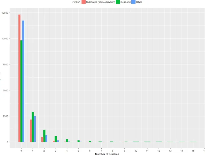
Yearly crash frequency data per direction for 1,506 urban midblock segments in Lincoln and Omaha, Nebraska from 2003 to 2012 were collected from the Nebraska Department of Roads. Originally, these midblock segments were selected by a technical committee from the Nebraska Department of Roads to investigate the effects of narrow lane width on urban roadway safety (Sharma et al., 2015), for which researchers focused mainly on regular vehicle crashes, and thus excluded animal crashes, alcohol-related crashes, crashes caused by road surface conditions, and heavy vehicle crashes. Sideswipe (same direction) and rear-end crashes made up 18.9% and 57.5% of the crash data, respectively, whereas most of the remaining crashes were recorded as not applicable. Thus, crashes were classified into three major types: sideswipe (same direction) crashes, rear-end crashes, and other crashes. The first two crash types were the focus of this study, but other crashes were still used in the modeling analysis, as it was believed that they might have some underlying correlations to the first two crash types, and could be utilized to better explore the characteristics of sideswipe (same direction) and rear-end crashes in multivariate models. In addition to crash data, many traffic operation and roadway geometric data were collected by field study and measurements in Google Earth. A summary of collected variables is given in Table 1. Each midblock segment was homogenous with respect to annual average daily traffic per lane, number of through lanes, median type, left-turn treatment, and other key factors. The annual average daily traffic per lane per direction for each segment was obtained from the Nebraska Department of Roads. The lane widths of these segments included 9-ft, 10-ft, 11-ft, and 12-ft widths, and 12-ft width was used as the baseline lane width in modeling. The speed limits for these segments included 25 mph, 35 mph, 40 mph, and 45 mph, and 25 mph was used as the baseline speed limit in modeling. These segments were also classified into four groups by the National Functional Classification (NFC) system (Federal Highway Administration, 2013): NFC-14, urban principal arterial–other connecting link; NFC-15, urban principal arterial–other non-connecting link; NFC-16, urban minor arterial; and NFC-17, urban collector. NFC-17 was used as the baseline roadway class in modeling.
Variances of all three crash types were larger than their means, as shown in Table 1, which implies that over dispersion existed for all of them. The percentages of zero values of sideswipe (same direction), rear-end, and other crash types were 81.4%, 65.2%, and 77.6%, respectively, larger than the expected probabilities of zero values (78.7%, 48.5%, and 74.1%, respectively) of Poisson distributions with means of 0.240, 0.724, and 0.300, respectively. This indicated that excess zeros existed for all three crash types, which also could be visualized in the histograms of crash data in Figure 1.
Table 1 Descriptive statistics of collected variables
Name Description Mean
Std.
err. Min. Max.
Zero-proportion
Sideswipe (same direction)
Number of sideswipe (same direction) crashes per direction per segment per year
0.240 0.568 0 9 81.4%
Rear-end Number of rear-end crashes per
direction per segment per year 0.724 1.576 0 43 65.2%
Others Number of rest crashes per direction
per segment per year 0.300 0.641 0 8 77.6%
Independent variables
Number of lanes Number of through lanes 1.929 0.005 1 6
Annual average daily traffic
per lane 1,000 vehicles 5.668 0.019 0.100 13.975
Segment length Miles 0.363 0.002 0.025 2.003
Shoulder indicator 1, shoulder exists (25.4%); 0, no shoulder (74.6%) Median indicator 1, median exists (79.5%); 0, no median (20.5%)
On-street parking indicator 1, on-street parking exists (5.6%); 0, no on-street parking (94.4%) Central business district
indicator
1, in central business district (6.1%); 0, out of central business district (93.9%)
One-way road indicator 1, roadway is one-way (3.7%); 0, roadway is two-way (96.3%) Lane width Feet (ft): 9 ft (3.1%); 10 ft (15.5%); 11 ft (29.8%); 12 ft (51.6%) Lane width – 9 ft indicator 1, lane width is 9 ft; 0, otherwise
Lane width – 10 ft indicator 1, lane width is 10 ft; 0, otherwise Lane width – 11 ft indicator 1, lane width is 11 ft; 0, otherwise
Speed limit Mph: 25 (6.0%); 35 (32.6%); 40 (30.7%); 45 (30.7%)
Speed limit – 35 mph indicator 1, speed limit is 35 mph; 0, otherwise Speed limit – 40 mph indicator 1, speed limit is 40 mph; 0, otherwise Speed limit – 45 mph indicator 1, speed limit is 45 mph; 0, otherwise
National functional
classification (NFC)
NFC-14: urban principal arterial–other connecting link, 13.9%; NFC-15: urban principal arterial–other non-connecting link, 37.6%; NFC-16: urban minor arterial, 41.2%;
NFC-17: major collector, 7.3%.
NFC-14 indicator 1, segment belongs to NFC-14; 0, otherwise
NFC-15 indicator 1, segment belongs to NFC-15; 0, otherwise
NFC-16 indicator 1, segment belongs to NFC-16; 0, otherwise
Figure 1 Histogram of sideswipe (same direction), rear-end, and other crash types from 2003 to 2012
4
RESULTS AND DISCUSSIONS
Out of the 10 years of data, data from 2003 to 2011 were used for the model estimation, and the 2012 data were used for prediction.
4.1 Model Comparison
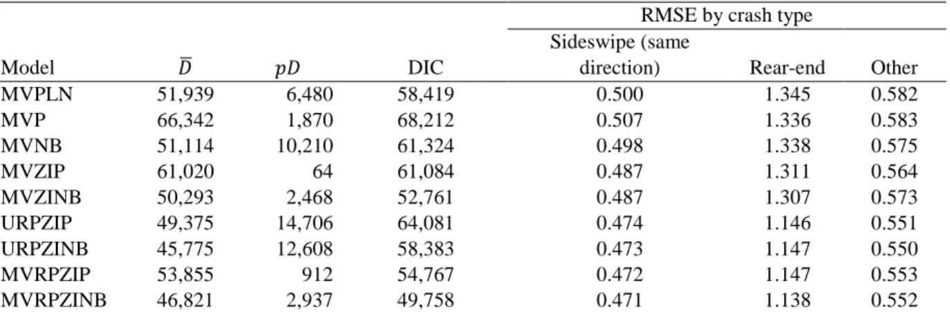
In addition to the multivariate random parameters zero-inflated negative binomial model, the multivariate Poisson log-normal model, the univariate random parameters zero-inflated Poisson model, the univariate random parameters zero-inflated negative binomial model, the multivariate zero-inflated Poisson model, the multivariate zero-inflated negative binomial model, and the multivariate random parameters zero-inflated Poisson model were also estimated for comparison. The DIC and RMSE values of these models are shown in Table 2.
Table 2 DIC and RMSE values for all the estimated models
Model DIC
RMSE by crash type
𝐷𝐷� 𝑝𝑝𝐷𝐷
Sideswipe (same
direction) Rear-end Other
MVPLN 51,939 6,480 58,419 0.500 1.345 0.582 MVP 66,342 1,870 68,212 0.507 1.336 0.583 MVNB 51,114 10,210 61,324 0.498 1.338 0.575 MVZIP 61,020 64 61,084 0.487 1.311 0.564 MVZINB 50,293 2,468 52,761 0.487 1.307 0.573 URPZIP 49,375 14,706 64,081 0.474 1.146 0.551 URPZINB 45,775 12,608 58,383 0.473 1.147 0.550 MVRPZIP 53,855 912 54,767 0.472 1.147 0.553 MVRPZINB 46,821 2,937 49,758 0.471 1.138 0.552
Note: DIC, Deviance information criteria; RMSE, root mean square error; 𝐷𝐷�, mean of the sampled deviances from Markov-chain Monte Carlo simulations; 𝑝𝑝𝐷𝐷, effective number of parameters in the model; MVPLN, multivariate Poisson log-normal; MVP, multivariate Poisson; MVNB, multivariate negative binomial; MVZIP, multivariate zero-inflated Poisson; MVZINB, multivariate zero-zero-inflated negative binomial; URPZIP, univariate random parameters zero-inflated Poisson; URPZINB, univariate random parameters zero-inflated negative binomial; MVRPZIP, multivariate random parameters zero-inflated Poisson; MVRPZINB, multivariate random parameters zero-inflated negative binomial.
From Table 2, the following observations can be made:
1. DIC and RMSE values of the multivariate random parameters zero-inflated negative binomial model were generally much lower than those of all the other models, showing its superiority. 2. Compared to the multivariate Poisson/negative binomial models, the multivariate zero-inflated Poisson/negative binomial models had much smaller DIC and RMSE values, respectively, which shows the superiority of multivariate zero-inflated models for analyzing the multivariate crash data with excess zeros.
3. Compared to the multivariate zero-inflated Poisson/negative binomial models, the multivariate random parameters zero-inflated Poisson/negative binomial models showed much better performance in terms of DIC and RMSE. Although the multivariate zero-inflated Poisson/negative binomial models had lower 𝑝𝑝𝐷𝐷values, their 𝐷𝐷� values were much higher. This means that the multivariate random parameters zero-inflated Poisson/negative binomial models are more complex but fit the data much better. The result is straightforward, as the random parameters models allow estimated parameters to vary across segments to account for unobserved heterogeneity. This flexibility improves the model’s ability to fit the data. This finding reiterates that the unobserved heterogeneity across observations in crash analyses may not be ignored (Mannering et al., 2016).
4. The RMSE values of the univariate random parameters zero-inflated Poisson/negative binomial models and the multivariate random parameters zero-inflated Poisson/negative binomial models were similar, but the latter models had much lower DIC values. The univariate random parameters zero-inflated Poisson/negative binomial models had relatively lower 𝐷𝐷� but much higher 𝑝𝑝𝐷𝐷 values, which indicated that they fit the data better but were more complex. As mentioned above, the multivariate models could account for unobserved heterogeneity across crash types. By
borrowing from the strength of between-crash correlations, multivariate models could estimate parameters more accurately than univariate models. This result shows the importance of multivariate modeling in analysis of multiple crash types.
5. All the negative binomial models had much lower DIC values than did their corresponding Poisson models, but their RMSE values were very close, such as the multivariate random parameters zero-inflated Poisson model versus the multivariate random parameters zero-inflated negative binomial model. Considering that the only difference between the negative binomial models and their Poisson counterparts was that the negative binomial models had dispersion parameters but the Poisson models did not, the results suggest that the estimated parameters of the Poisson and negative binomial models were similar except for the dispersion parameters. The negative binomial models fit the data much better, as they could account for over dispersion of crash data. The results highlight that, although random parameters and zero-inflated models can also account for over dispersion to some degree, they might not cover all of it. It may be still necessary to specifically take over dispersion into account in crash frequency analyses.
6. The most popular multivariate count data model, the multivariate Poisson log-normal model, performed worse than the multivariate zero-inflated negative binomial model did in terms of both DIC and RMSE. Because Dong et al. (2014b) showed that the multivariate zero-inflated Poisson model was superior to the multivariate Poisson log-normal model for their dataset, it was believed that the multivariate zero-inflated count data models were competitive alternatives to the multivariate Poisson log-normal model for analyzing the multivariate zero-inflated data.
In general, as shown in Table 2, unobserved heterogeneity stemmed from the correlations across crash types, the correlations across segments, excess zeros, and over dispersion for the studied dataset, and none of them can be ignored. The multivariate random parameters zero-inflated negative binomial model was superior to other models as it could account for various unobserved heterogeneities.
Because many independent variables were found to be not significant for the multivariate random parameters zero-inflated negative binomial model, it was re-run after removing those nonsignificant variables, and the results are discussed in the following analysis.
4.2 Parameter Interpretation
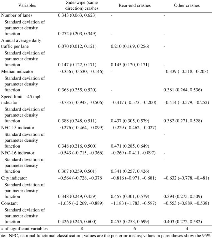
The means and 95% credible intervals of the estimated parameters of sideswipe (same direction), rear-end, and other crashes count parts of the multivariate random parameters zero-inflated negative binomial model and the multivariate zero-inflated negative binomial models are shown in Table 3 and Table 4, respectively. For the multivariate random parameters zero-inflated negative binomial model, if the standard deviation of parameter density function is statistically not significant, that parameter would be fixed. Probabilities of estimated parameters being negative and average marginal effects of the multivariate random parameters zero-inflated negative binomial model are shown in Table 5 and Table 6, respectively. Only significant variables are shown in these tables, and only the variables with both means and standard deviations significant were considered to be significant.
Table 3 Posterior summary (means and 95% credible intervals) of estimated parameters of the count part of the multivariate random parameters zero-inflated negative binomial model
Variables Sideswipe (same
direction) crashes Rear-end crashes Other crashes
Number of lanes 0.343 (0.063, 0.623) - -
Standard deviation of parameter density
function 0.272 (0.203, 0.349) - -
Annual average daily
traffic per lane 0.070 (0.012, 0.121) 0.210 (0.169, 0.256) -
Standard deviation of parameter density function 0.147 (0.122, 0.171) 0.145 (0.120, 0.171) - Median indicator –0.356 (–0.530, –0.146) - –0.339 (–0.518, -0.203) Standard deviation of parameter density function 0.368 (0.255, 0.520) - 0.381 (0.264, 0.536) Speed limit – 45 mph indicator –0.735 (–0.943, –0.506) –0.417 (–0.573, –0.200) –0.414 (–0.579, –0.252) Standard deviation of parameter density function 0.388 (0.248, 0.511) 0.437 (0.305, 0.579) 0.382 (0.271, 0.528) NFC-15 indicator –0.276 (–0.464, –0.099) –0.229 (–0.462, –0.027) - Standard deviation of parameter density function 0.348 (0.216, 0.500) 0.471 (0.285, 0.649) - NFC-16 indicator –0.543 (–0.715, –0.366) –0.269 (–0.411, -0.097) - Standard deviation of parameter density function 0.367 (0.259, 0.501) 0.341 (0.257, 0.426) - City indicator –0.564 (–0.728, –0.378 –0.816 (–0.971, –0.681) –0.632 (–0.778, –0.481) Standard deviation of parameter density function 0.348 (0.249, 0.459) 0.457 (0.301, 0.579) 0.394 (0.275, 0.509) Constant –1.635 (–2.269, –0.889) –1.183 (–1.783, –0.597) –0.553 (–0.889, –0.538) Standard deviation of parameter density function 0.426 (0.245, 0.600) 0.455 (0.253, 0.699) 0.403 (0.272, 0.582) # of significant variables 8 6 4
Note: NFC, national functional classification; values are the posterior means; values in parentheses show the 95% credible intervals; “-”, insignificant variables at the 95% credible level; shoulder indicator, on-street parking indicator, central business district indicator, segment length, one-way indicator, lane width (9 ft, 10 ft, and 11 ft) indicators, speed limit - 35 mph indicator, speed limit - 40 mph indicator, and NFC-14 indicator were not significant variables at the 95% credible level for any crash type.
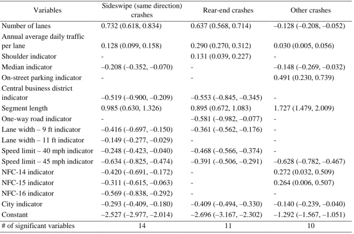
Table 4 Posterior summary (means and 95% credible intervals) of estimated parameters of the count part of the multivariate zero-inflated negative binomial model
Variables Sideswipe (same direction)
crashes Rear-end crashes Other crashes
Number of lanes 0.732 (0.618, 0.834) 0.637 (0.568, 0.714) –0.128 (–0.208, –0.052)
Annual average daily traffic
per lane 0.128 (0.099, 0.158) 0.290 (0.270, 0.312) 0.030 (0.005, 0.056)
Shoulder indicator - 0.131 (0.039, 0.227) -
Median indicator –0.208 (–0.352, –0.070) - –0.148 (–0.269, –0.032)
On-street parking indicator - - 0.491 (0.230, 0.739)
Central business district
indicator –0.519 (–0.900, –0.209) –0.553 (–0.845, –0.345) -
Segment length 0.985 (0.630, 1.326) 0.895 (0.672, 1.083) 1.727 (1.479, 2.009)
One-way road indicator - –0.581 (–0.982, –0.077) -
Lane width – 9 ft indicator –0.416 (–0.697, –0.150) –0.361 (–0.562, –0.176) -
Lane width – 11 ft indicator –0.149 (–0.277, –0.029) - -
Speed limit – 40 mph indicator –0.248 (–0.423, –0.040) –0.468 (–0.566, –0.374) -
Speed limit – 45 mph indicator –0.634 (–0.825, –0.474) –0.391 (–0.506, –0.291) –0.628 (–0.782, –0.467)
NFC-14 indicator –0.420 (–0.691, –0.172) - 0.272 (0.032, 0.509) NFC-15 indicator –0.311 (–0.615, –0.063) - 0.264 (0.006, 0.507) NFC-16 indicator –0.569 (–0.838, –0.292) - - City indicator –0.293 (–0.409, –0.180) –0.409 (–0.494, –0.330) –0.140 (–0.239, –0.040) Constant –2.527 (–2.977, –2.014) –2.696 (–3.167, –2.302) –1.292 (–1.567, –1.051) # of significant variables 14 11 10
Note: NFC, national functional classification; values are the posterior means; values in parentheses show the 95% credible intervals; “-”, insignificant variables at the 95% credible level; lane width – 10ft indicator and speed limit – 35 mph indicator were not significant variables at the 95% credible level for any crash type.
Table 5 Probabilities of the estimated parameters being negative for the count part of the multivariate random parameters zero-inflated negative binomial model
Variables Sideswipe (same direction) crashes Rear-end crashes Other crashes
Number of lanes 0.104 - -
Annual average daily traffic per
lane 0.317
0.074 -
Median indicator 0.833 - 0.813
Speed limit – 45 mph indicator 0.971 0.830 0.861
NFC-15 indicator 0.786 0.687 -
NFC-16 indicator 0.931 0.785 -
City indicator 0.947 0.963 0.946
Note: NFC, national functional classification; “-”, insignificant variables at the 95% credible level; shoulder indicator, on-street parking indicator, central business district indicator, segment length, one-way indicator, lane width (9 ft, 10 ft, and 11 ft) indicators, speed limit – 35 mph indicator, speed limit – 40 mph indicator , and NFC-14 indicator were not significant variables at the 95% credible level for any crash type.
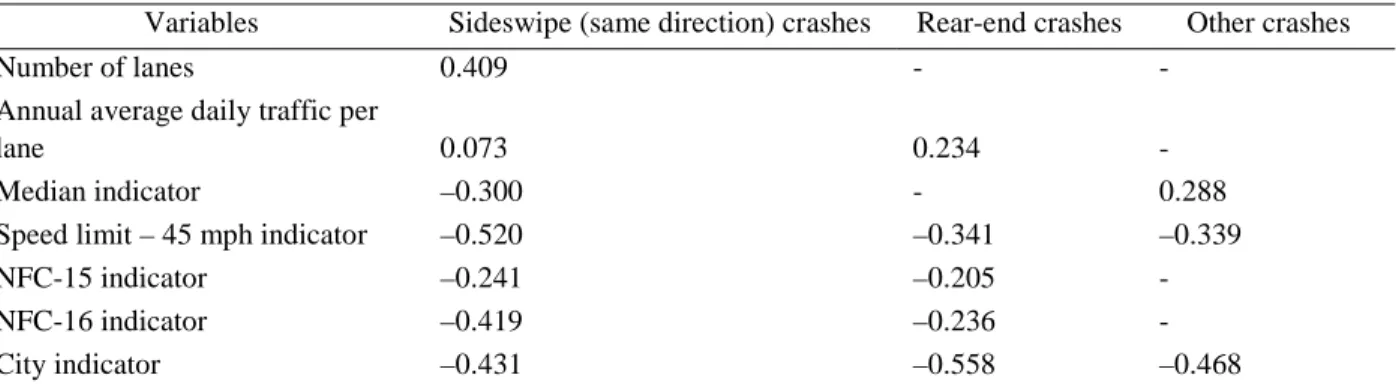
Table 6 Average marginal effects of the count part of the multivariate random parameters zero-inflated negative binomial model
Variables Sideswipe (same direction) crashes Rear-end crashes Other crashes
Number of lanes 0.409 - -
Annual average daily traffic per
lane 0.073 0.234 -
Median indicator –0.300 - 0.288
Speed limit – 45 mph indicator –0.520 –0.341 –0.339
NFC-15 indicator –0.241 –0.205 -
NFC-16 indicator –0.419 –0.236 -
City indicator –0.431 –0.558 –0.468
Note: NFC, national functional classification; “-”, nonsignificant variables at the 95% credible level shoulder indicator, on-street parking indicator, central business district indicator, segment length, one-way indicator, lane width (9 ft, 10 ft, and 11 ft) indicators, speed limit – 35 mph indicator, speed limit – 40 mph indicator, and NFC-14 indicator were not significant variables at the 95% credible level for any crash type.
Number of lanes showed significant effects only for sideswipe (same direction) crashes. When the number of lanes increased, 89.6% of segments had more sideswipe (same direction) crashes, and on average, the number of sideswipe (same direction) crashes increased 40.9% with a one lane increase. This finding is reasonable, as with more lanes, vehicles have more opportunities to travel parallel to each other on segments. In addition, 10.4% of segments tended to have fewer sideswipe (same direction) crashes with an increase in the number of lanes. Number of lanes did not show significant effects on rear-end or other crash types. Although more lanes might bring more traffic, drivers also have more space to maneuver to avoid crashes and they may also drive more carefully. Thus, these effects might offset each other.
Annual average daily traffic has been widely found to have a positive effect on crash frequency when it is assumed to have a fixed effect (Bonneson and Mccoy, 1997; Greibe, 2003; Zhang et al., 2012; Dong et al., 2014a, 2014b; Ferreira and Couto, 2015); however, this may not always be true. In this study, annual average daily traffic per lane showed a significant influence on the number of sideswipe (same direction) and rear-end crashes. The estimated parameters were normally distributed with a mean of 0.070 (standard deviation of parameter density function = 0.147) for the sideswipe (same direction) crash and a mean of 0.210 (standard deviation of parameter density function = 0.145) for the rear-end crash. On average, the numbers of sideswipe (same direction) and rear-end crashes increased by 7.3% and 23.4%, respectively, as annual average daily traffic per lane increased by 1,000 vehicles. Even though the number of sideswipe (same direction) and rear-end crashes increased for most segments with an increase of annual average daily traffic per lane, these numbers decreased for 31.7% and 7.4% of segments, respectively. Although an increase in annual average daily traffic per lane increases crash opportunities, it could also provide some underlying safety effects, such as more cautious driving, intensive traffic enforcement, and advanced traffic control devices, which could offset the increased crash risk. Thus, the increase in annual average daily traffic per lane did not necessarily increase the number of crashes. However, this does not mean that crash frequencies would not increase or even decrease with a continuing
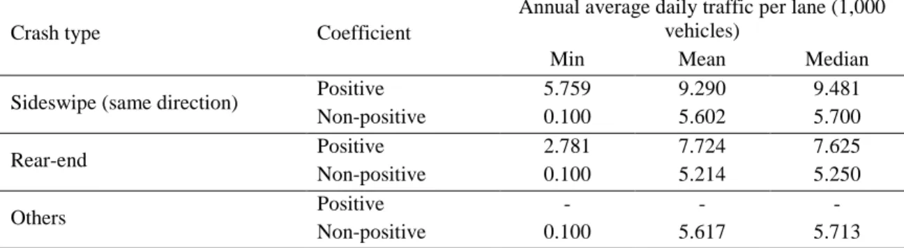
increase of annual average daily traffic per lane. A summary of annual average daily traffic per lane by crash types and signs of estimated regression coefficients is shown in Table 7. The segments with positive coefficients for annual average daily traffic per lane generally had much higher annual average daily traffic per lane than did those with non-positive coefficients. That is, for segments already with very high annual average daily traffic per lane, the crash frequency was more likely to increase with an increase of annual average daily traffic per lane. In addition, it should be noted that segments with non-positive coefficients of annual average daily traffic per lane for all three crash types had a mean annual average daily traffic per lane value of around 5.5, which seemed an important threshold. Mannering et al. (2016) proposed that there might be heterogeneous linear or non-linear relationships between traffic volume and accident likelihood, which is proved somewhat by this study. Anastasopoulos (2016) also showed that, using the multivariate random parameters zero-inflated negative binomial model, annual average daily traffic had inconsistent influences on crash frequencies for roadway segments in Indiana.
Table 7 Summary of annual average daily traffic per lane by crash types and signs of regression coefficients
Crash type Coefficient
Annual average daily traffic per lane (1,000 vehicles)
Min Mean Median
Sideswipe (same direction) Positive 5.759 9.290 9.481
Non-positive 0.100 5.602 5.700 Rear-end Positive 2.781 7.724 7.625 Non-positive 0.100 5.214 5.250 Others Positive - - - Non-positive 0.100 5.617 5.713 Note: “-”, unavailable.
Segment length did not show a significant influence on any crash type. Most segments studied were very short, the average segment length being 0.363 mile and 75.6% of segments being shorter than 0.5 mile. It is thought that these segment lengths might not be different enough to show significant effects.
It should be noted that crash frequency is usually assumed to increase with an increase in the number of lanes, annual average daily traffic, and segment length; thus, many studies have used these variables as exposure variables (Miaou et al., 2003; Miaou and Song, 2005; Boulieri et al., 2017). As presented in Table 4, the estimated parameters of the multivariate zero-inflated negative binomial model are generally consistent with these beliefs, whereby number of lanes, annual average daily traffic per lane, and segment length showed positive effects on all crash types, except for number of lanes for other crash types. The inconsistent findings of the multivariate zero-inflated negative binomial model and the multivariate random parameters zero-zero-inflated negative binomial models show the advantage of random parameter models that they can capture the segment-specific effects, which are unavailable in fixed parameter models but very important, especially when opposite segment-specific effects exist. This also suggests that researchers should be very careful in using these variables as exposure variables, as the precondition might be violated.
The presence of a shoulder had no significant influence on any crash type. For freeways or rural highways, the shoulder is very important in the event of emergency or breakdown. However, on urban arterials, these events may not interrupt traffic seriously due to lower travel speeds, better roadway lighting, and more access points for leaving the roadway. Thus, the lack of a shoulder may not have influenced traffic safety for the studied roadways. The results are consistent with the study by Zhao et al. (2017), who found that a shoulder did not have significant effects on crash frequencies of urban signalized intersection approaches in either Lincoln or Omaha, Nebraska. However, the presence of a median had a significant influence on the number of sideswipe (same direction) crashes with a mean of –0.356 (standard deviation of parameter density function = 0.368), and other crashes with a mean of –0.339 (standard deviation of parameter density function = 0.381). When a median was present, 83.3% and 81.3% of segments had fewer sideswipe (same direction) and other crash types, respectively. On average, the number of sideswipe (same direction) and other crash types decreased by 30.0% and 28.8%, respectively. When a road median is present, left-turn and U-turn traffic is expected to decrease, leading to fewer sideswipe (same direction) collisions. This could also reduce sideswipe (opposite direction) crashes, angle crashes, and so on, which may explain why the number of other crash types decreased for most segments. However, the number of vehicle collisions with medians may increase; thus, some segments might have more crashes.
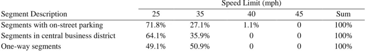
The presence of on-street parking, being in a central business district, or one-way traffic did not show significant influence on the number of any crash type. The speed limit characteristics of segments with on-street parking, in a central business district, or with one-way traffic are shown in Table 8. Most of these segments had speed limits of 25 mph or 35 mph. Under such low-speed environments, these factors would not be expected to pose significant threats to traffic safety.
Table 8 Speed limits of segments with on-street parking, segments in central business district, and one-way traffic
Speed Limit (mph)
Segment Description 25 35 40 45 Sum
Segments with on-street parking 71.8% 27.1% 1.1% 0 100%
Segments in central business district 64.1% 35.9% 0 0 100%
One-way segments 49.1% 50.9% 0 0 100%
Narrow lanes are often needed in cities to accommodate parking, bike lanes, sidewalks, drainage, and utilities. Although it is intuitive that providing some buffer space might prevent the occurrences of crashes, past studies evaluating the impact of narrower lane width on urban roadway safety have revealed inconsistent results: negative effects (Harwood, 1990), non-linear effects (Lee et al., 2015; Park and Abdel-Aty, 2016), and no effects (Potts et al., 2007). The multivariate random parameters zero-inflated negative binomial model showed that lane width did not have a significant influence on any crash type in this dataset. Although narrow lanes might increase the opportunities for some collision types, such as sideswipe (same direction) crashes, they might also have lower speed limits, less traffic, and less aggressive driving. The net effect of these opposite forces determines the impact of narrow lanes on crash frequency. The findings of
this study suggest that, for the studied roadways, safety might not be a concern if lanes need to be made narrower to accommodate other street elements.
Compared with a 25-mph speed limit, 35-mph and 40-mph speed limits did not show significant influences on midblock crash frequencies, but a 45-mph speed limit did show significant effects. For the 45-mph speed limit, the estimated normally distributed parameters had a mean of –0.735 (standard deviation of parameter density function = 0.388) for sideswipe (same direction) crashes, a mean of –0.417 (standard deviation of parameter density function = 0.437) for rear-end crashes, and a mean of –0.414 (standard deviation of parameter density function = 0.382) for other crash types. That is, 97.1%, 83.0%, and 86.1% of the segments tended to have fewer sideswipe (same direction), rear-end, and other crashes, respectively, with a 45-mph speed limit than with lower speed limits. Simultaneously, only 2.9%, 17.0%, and 13.9% of segments tended to have more sideswipe (same direction), rear-end, and other crash types, respectively. Intuitively, it would seem that higher speed limits would increase the probability of crashes occurring, but roadways with high speed limits usually have fewer access roads and better designed facilities. Thus, it appears that the advantages of high speed limits outweighed the disadvantages for most segments. On average, sideswipe (same direction), rear-end, and other crash types decreased by 52.0%, 34.1%, and 33.9%, respectively, on segments with a 45-mph speed limit compared with those with lower speed limits. This study’s findings suggest that 45 mph is an important threshold in determining speed limits for urban arterials. For the multivariate zero-inflated negative binomial model, the speed limit was also found to have negative effects on all crashes. However, although an increased speed limit might reduce the number of crashes and increase capacity for most segments, it might also increase the severity of crash damage and injuries (Renski et al., 1999; Malyshkina and Mannering, 2008), as the outcomes of high-speed object collisions are more serious. Thus, speed limit increases should be carefully studied before implementation.
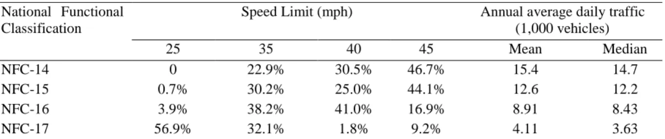
Compared with major collectors (NFC-17), urban principal arterial–other non-connecting link (NFC-15) and urban minor arterial (NFC-16) showed significant influences on the number of sideswipe (same direction) and rear-end crashes. Compared to NFC-17 segments, 78.6% and 86.7% of NFC-15 segments had fewer sideswipe (same direction) and rear-end crashes, respectively, and 93.1% and 78.5% of NFC-16 segments had fewer sideswipe (same direction) and rear-end crashes, respectively. Speed limit compositions, as well as mean and median annual average daily traffic values of segments by functional classification, are shown in Table 9. The mean speed limits of NFC-15 and NFC-16 segments were higher than those of NFC-17 segments, and it was proved above that the number of crashes tended to decrease with higher speed limits. Thus, this might explain why most NFC-15 and NFC-16 segments tended to have fewer crashes. However, urban principal arterial–other connecting link (NFC-14) segments did not show significant influences on any crash type, although they had the highest speed limits. A possible explanation is that the NFC-14 segments also had very large annual average daily traffic values, which probably led to the occurrence of more crashes. These factors might play different roles for segments by functional classification, leading to different results. In addition, speed limit and annual average daily traffic reflect the mobility function of roadways, whereas accessibility is another function in determining NFC levels for roadways (Federal Highway Administration,
2013). Although accessibility information was unavailable in this dataset, it may also influence crash frequencies.
Table 9 Speed limit compositions, and mean and median annual average daily traffic values of segments by national function classification
National Functional Classification
Speed Limit (mph) Annual average daily traffic
(1,000 vehicles) 25 35 40 45 Mean Median NFC-14 0 22.9% 30.5% 46.7% 15.4 14.7 NFC-15 0.7% 30.2% 25.0% 44.1% 12.6 12.2 NFC-16 3.9% 38.2% 41.0% 16.9% 8.91 8.43 NFC-17 56.9% 32.1% 1.8% 9.2% 4.11 3.63
Note: NFC, national functional classification.
The city i (Lincoln vs. Omaha) showed a significant influence on all crash types. The estimated normally distributed parameters had a mean of –0.564 (standard deviation of parameter density function = 0.348) for sideswipe (same direction) crashes, a mean of –0.816 (standard deviation of parameter density function = 0.457) for rear-end crashes, and a mean of –0.632 (standard deviation of parameter density function = 0.394) for other crash types. The probabilities of the city variable being negative were 86.3%, 95.1%, and 90.7% for the three crash types, respectively. The number of sideswipe (same direction), rear-end, and other crashes for segments in Omaha were lower than those in Lincoln by an average of 25.4%, 33.6%, and 13.1%, respectively, when other characteristics were same. It should be noted that signalized intersection approaches in Omaha were also found to have fewer crashes than did those in Lincoln (Zhao et al., 2017). Considering that Lincoln and Omaha are only 45-min driving time apart, driving behaviors in the two cities are expected to be similar. Thus, some other features, such as traffic enforcement, land use, and terrain, might be responsible for this difference. Further studies are needed to investigate the true reasons, which would be very helpful for transportation agencies in formulating accurate countermeasures to improve traffic safety in Lincoln.
The estimated parameters of the inflation part of the multivariate random parameters zero-inflated negative binomial model and the multivariate zero-zero-inflated negative binomial models are shown in Table 10 and Table 11, respectively. Although both models adopted fixed parameters for the zero-inflation part, their significant variables were very different due to different count part models. This indicates that, for zero-inflated models, the count parts and zero-inflated parts were highly correlated and that a modeling framework change in one part would greatly influence the result of the other part. For both models, the number of lanes, annual average daily traffic per lane, and segment length showed significantly negative effects on the number of some crash types, which means that with the increase of the values of these covariates, these crash types were less likely to have zero values. That is, the expected crash frequencies would increase. It is reasonable to infer, as has been proved, that for most segments, these covariates have positive effects on crash frequencies. In addition, a 45-mph speed limit showed significant positive effect on the number of sideswipe (same direction) crashes for the multivariate random parameters zero-inflated negative binomial model, which means that zero crashes were more likely to appear under the 45-mph speed
limit. This result is also consistent with the results of the count part of the multivariate random parameters zero-inflated negative binomial model.
Out of total 18 covariates, 9 and 16 covariates were found to be significant (at least in either the count part or the zero-inflation part) for the multivariate random parameters zero-inflated negative binomial model and the multivariate zero-inflated negative binomial model, respectively. That is, the multivariate random parameters zero-inflated negative binomial model showed a much better performance with fewer variables than did the multivariate zero-inflated negative binomial model in this case, which was helpful for identifying critical crash-influencing factors. However, this may not be true in other cases, as in the study by Dong et al. (2014a), the multivariate random parameters zero-inflated negative binomial model identified more significant factors than did the multivariate zero-inflated negative binomial model.
Table 10 Posterior summary (means and 95% credible intervals) of estimated parameters of the zero-inflation part of the multivariate random parameters zero-inflated negative binomial model
Variables Sideswipe (same direction)
crashes Rear–end crashes Other crashes
Number of lanes - - –5.823 (-8.643, –3.684)
Annual average daily
traffic per lane –1.192 (–1.664, –0.719) - –0.331 (–0.571, –0.091)
Median indicator - 1.990 (0.039, 5.466) -
Central business district
indicator - –7.451 (–13.851, -1.680) - Segment length –13.512 (–18.672, –8.768) –17.910 (–26.774, –10.887) - Speed limit – 45 mph indicator 2.647 (1.007, 4.272) - - NFC-15 indicator - - –2.727 (–5.703, –0.047) NFC-16 indicator 5.419 (1.154, 12.108) 2.730 (0.121, 6.440) –4.615 (–7.680, –2.202) City indicator –5.874 (–10.602, –1.451) - - Constant - - 7.696 (5.119, 10.595) # of significant variables 6 4 5
Note: NFC, national functional classification; values shown are posterior means; values in parentheses show the 95% credible intervals; “-”, nonsignificant variables at the 95% credible level. Shoulder indicator, on-street parking indicator, one-way indicator, lane width (9ft, 10ft, and 11ft) indicators, speed limit – 35mph indicator, speed limit – 40mph indicator, and NFC-14 indicator were not significant variables at the 95% credible level for any crash type.
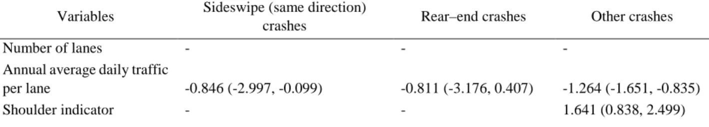
Table 11 Posterior summary (means and 95% credible intervals) of estimated parameters of the zero-inflation part of the multivariate zero-inflated negative binomial model
Variables Sideswipe (same direction)
crashes Rear–end crashes Other crashes
Number of lanes - - -
Annual average daily traffic
per lane -0.846 (-2.997, -0.099) -0.811 (-3.176, 0.407) -1.264 (-1.651, -0.835)
Median indicator 2.858 (1.103, 4.912) - - Segment length -7.934 (-11.899, -0.064) - - Lane width – 10 ft indicator - - 1.152 (0.128, 2.179) NFC - 16 indicator - - -1.744 (-2.933, -0.550) # of significant variables 4 1 4
Note: NFC, national functional classification; values shown are posterior means; values in parentheses show the 95% credible intervals; “-”, nonsignificant variables at the 95% credible level. On-street parking indicator, central business district indicator, one-way indicator, lane width – 9ft indicator, lane width – 11ft indicator, speed limit (35mph, 40mph, and 45mph) indicators, NFC-14 indicator, and NFC-15 indicator, city indicator, and number of lanes were not significant variables at the 95% credible level for any crash type.
5
CONCLUSIONS
In this study, we analyzed sideswipe (same direction), rear-end, and other crash types over 10 years (2003–2012) on 1,506 urban midblock segments in Lincoln and Omaha, Nebraska. Traffic operation and roadway geometry characteristics were investigated to identify significant influencing factors. Due to the concern of unobserved heterogeneity produced by correlations across crash types and segments, excess zeros, and over dispersion in crash data, the multivariate random parameters zero-inflated negative binomial model was used to simultaneously analyze these crashes. Compared to the multivariate Poisson log-normal, univariate random parameters zero-inflated Poisson, univariate random parameters zero-inflated negative binomial, multivariate zero-inflated Poisson, multivariate zero-inflated negative binomial and multivariate random parameters zero-inflated Poisson models, the multivariate random parameters zero-inflated negative binomial model provided a better fit in terms of both DIC and RMSE values for all three crash types. The model comparison showed that none of the four types of unobserved heterogeneities was negligible. The results proved the necessity and importance of using the multivariate random parameters zero-inflated negative binomial model to analyze multivariate panel crash data with excess zeros.
The multivariate random parameters zero-inflated negative binomial model revealed 9 out of 18 covariates as significantly influencing crash frequency for the studied midblock segments. The multivariate random parameters zero-inflated negative binomial model showed that number of lanes, annual average daily traffic per lane, and segment length might have non-positive effects on crash frequencies for some segments. Thus, in future studies, care should be taken in using them as exposure variables. Segments with a speed limit of 45 mph tended to have fewer crashes than did those with lower speed limits, and the segments in Omaha tended to have fewer crashes than did those in Lincoln. It was also found that the presence of a shoulder, central business district, on-street parking, and one-way traffic, as well as lane width, did not have significant influences on crash frequencies. The multivariate random parameters zero-inflated negative binomial model also made it possible to explore influencing factors for individual segments. These findings are informative for transportation agencies as they seek to take correct and efficient measures to improve traffic safety. By contrast, the multivariate zero-inflated negative binomial model
produced results consistent with intuition, but the results may be insufficient to provide actionable recommendations. The multivariate random parameters zero-inflated negative binomial model found fewer significant factors than did the multivariate zero-inflated negative binomial model, which was helpful for identifying key factors.
Several aspects of this study could be further improved in future studies. First, the multivariate random parameters zero-inflated negative binomial model were estimated using MCMC, which was time consuming and required a large capacity to store MCMC samples. With an increase in the amount and dimensions of data, MCMC would become even more cumbersome. Thus, Bayesian approximation methods, such as Integrated Nested Laplace Approximation and Variational Bayes, should be explored to improve computing efficiency. Second, the complexity of the multivariate random parameters zero-inflated negative binomial model makes the results less interpretable. For example, the rear-end crash frequencies marginally followed the zero-inflated negative binomial distribution in the multivariate zero-zero-inflated negative binomial model. However, it would be very difficult to calculate the marginal effects of annual average daily traffic per lane on rear-end crash frequencies in the multivariate zero-inflated negative binomial model, as this involved both the count part and the zero-inflation part. It would be even more difficult for the random parameters models. Sensitivity analysis and easy-to-understand visualization tools might be good solutions for showing the intricate correlations between covariates and response variables. Third, as an alternative to traditional zero-inflated models, the zero-state Markov switching count data model could distinguish zero-accident state and normal-count state in a straightforward manner and, as well, could capture the state change over time (Malyshkina et al., 2009; Malyshkina and Mannering, 2010); however, it has never been used in multivariate or random parameters scenarios. Future studies may explore the performance of the multivariate random parameters zero-state Markov switching count data model in analyzing similar crash data. Finally, crash frequency data are aggregated over time and space. Thus, they may have some spatial and temporal correlations (Liu et al., 2015; Boulieri et al., 2017; Liu and Sharma, 2017, 2018; Ma et al., 2017), and the effects of explanatory variables may also be instable over space and time (Mannering, 2018), which should be considered in future studies. In addition, the dataset did not include information about pavement conditions and access points, which have been proved to be very important for segment crash frequencies in many studies (Usman et al., 2010; Lee et al., 2011; Xiong et al., 2014; Zeng and Huang, 2014). Future studies should collect these data to produce more accurate results.
REFERENCES
Aguero-Valverde, J., Jovanis, P.P., 2010. Bayesian multivariate Poisson lognormal models for crash severity modeling and site ranking. Transportation Research Record 2136, 82–91. Alarifi, S.A., Abdel-Aty, M.A., Lee, J., Park, J., 2017. Crash modeling for intersections and
segments along corridors: a Bayesian multilevel joint model with random parameters. Analytic Methods in Accident Research 16, 48–59.