A Combination of Multiperiod Training Data and Ensemble Methods in Churn Classification: the Case of Housing Loan Churn

(1)

A COMBINATION OF

MULTI-PERIOD TRAINING DATA AND

ENSEMBLE METHODS IN CHURN

CLASSIFICATION

THE CASE OF HOUSING LOAN CHURN

Master’s Thesis

Le Thuy

15 May 2017

Information and Service

Economy

Approved in the Department of Information and Service Economy __ / __ / 2017 and awarded the grade

(2)

www.aalto.fi Abstract of master’s thesis

Author Le Thuy

Title of thesis A COMBINATION OF MULTI-PERIOD TRAINING DATA AND ENSEMBLE

METHODS IN CHURN CLASSIFICATION

Degree Master of Science in Economics and Business Administration

Degree programme Information and Service Economy

Thesis advisor(s) Tomi Seppälä

Year of approval 2017 Number of pages 79 Language English

Abstract

Customer retention has been the focus of customer relationship management research in the financial sector during the past decade. The first step in customer retention is to classify the customers into binary groups of possible churners, meaning customers that are likely to switch to another service provider, and non-churners, referring to those that are probably staying with the current provider. The second step in customer retention is to take action to retain the most probable churners to either minimize costs or maximize benefits. As a result, churn classification is an important first step in customer retention.

However, the main challenge in churn classification is the extreme rarity of churn events. For example, the churn rate in the banking industry is usually less than 1%. In order to overcome this rarity issue, a great deal of research has been found to improve the two main aspects of a churn classification model: the training data and the algorithm. Regarding the training data, the recently proposed multi-period training data approach is found to outperform the single period training data thanks to the more effective use of longitudinal data of churn behavior. Regarding the churn classification algorithms, the most advanced and widely employed is ensemble method, which combines multiple models to produce a more powerful one. Two popularly used ensemble techniques are random forest and gradient boosting, both of which are found to outperform logistic regression and decision tree in classifying churners from non-churners.

To the best of the author’s knowledge, the proposed multi-period training data has not been applied to the ensemble methods in a churn classification model. As a result, the thesis would like to study whether this multi-period training data approach, when employed together with ensemble methods in a churn classification model, produces better churn prediction than with logistic regression and decision tree. The ensemble methods used in this thesis are random forest and gradient boosting.

The study uses empirical data of housing loan customers from a Nordic bank. The churn models are evaluated based on three criteria: misclassification rate, Receiver Operating Characteristics (ROC) index and top decile lift. The key finding of this thesis is models that combine multi-period training data approach with ensemble methods perform the best in the housing loan context based on the aforementioned evaluation criteria.

Keywords churn prediction, ensemble methods, random forest, gradient boosting, multiple

(3)

List of Figures

Figure 1: Thesis structure ... 8

Figure 2: Time window of analysis illustration for single period training data ... 13

Figure 3: Time windows of analysis illustration for single period training data and multi-period training data ... 14

Figure 4: Example of a ROC chart ... 24

Figure 5: Illustration of a lift chart ... 26

Figure 6: Illustration of bagging procedure in SAS Enterpsie Miner ... 31

Figure 7: Illustration of boosting procedure in SAS Enterprise Miner ... 31

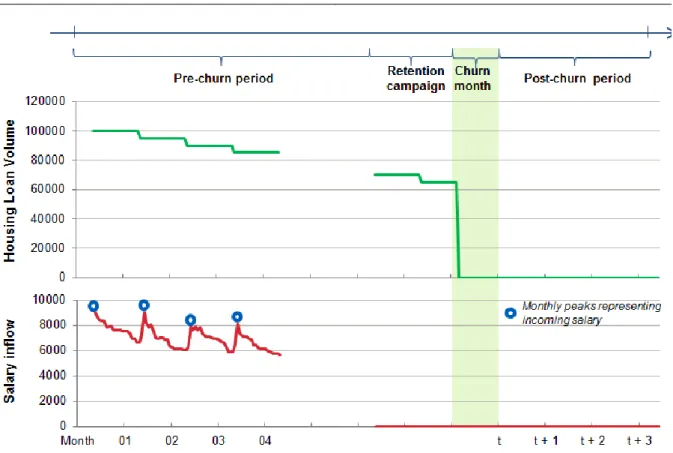
Figure 8: Illustration of the churn definition employed in this thesis ... 38

Figure 9: Time window of analysis for single period training data of churn in December 2015 ... 39

Figure 10: Time window of analysis for multi-period training data ... 40

Figure 11: Housing loan churn rates within the time window of anaylsis... 40

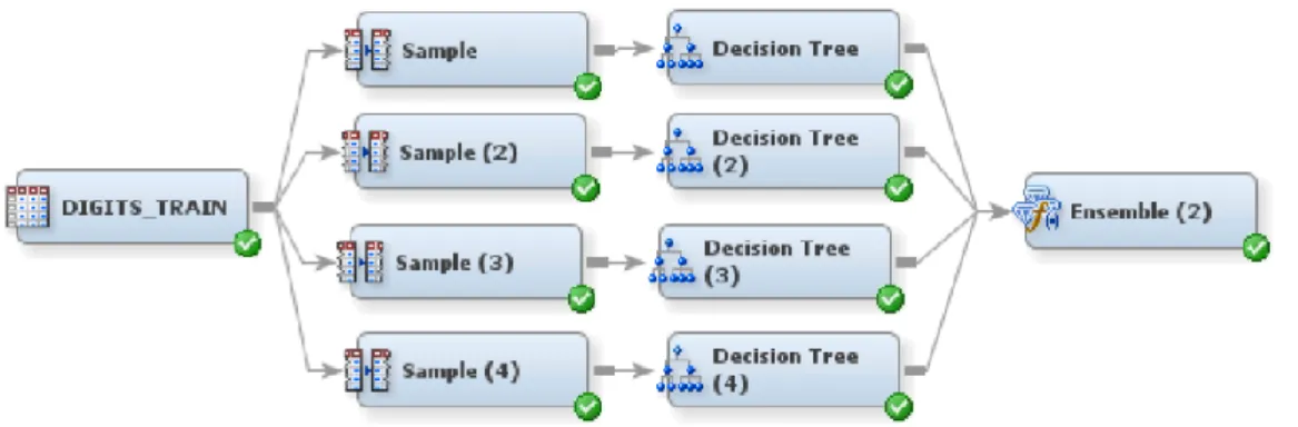
Figure 12: Modelling diagram in SAS Enterprise Miner 7.1... 48

Figure 13: Misclassification rate comparison between multi-period training data and single period training data for models with logistic regression and decision tree ... 49

Figure 14: ROC index comparison between multi-period training data and single period training data with models with logistic regression and decision tree ... 50

Figure 15: Top decile lift comparison between multi-period training data and single period training data for models with logistic regression and decision tree ... 51

Figure 16: Misclassification rate comparison between random forest & gradient boosting and logistic regression & decision tree for models with single period training data ... 52

Figure 17: ROC index comparison between random forest & gradient boosting and logistic regression & decision tree for models with single period training data ... 52

Figure 18: Top decile lift comparison between random forest & gradient boosting and logistic regression & decision tree for models with single period training data ... 53

Figure 19: Misclassification rate versus the number of trees for a random forest model ... 53

Figure 20: Misclassification rate against the iterations for a gradient boosting model ... 54

Figure 21: Misclassification rate comparison of the models with random forest & gradient boosting and multi-period training data against the other models ... 55

Figure 22: ROC index comparison comparison of the models with random forest & gradient boosting and multi-period training data against the other models ... 56

(6)

Figure 23: Top decile lift comparison comparison of the models with random forest & gradient boosting and multi-period training data against the other models ... 56 Figure 24: First split from a random decision tree model with multi-period training data ... 58

(7)

List of Tables

Table 1: An overview of several recent churn studies ... 10

Table 2: Confusion matrix of churn classification ... 22

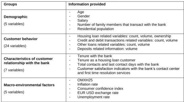
Table 3: List of churn predictors employed in this thesis ... 41

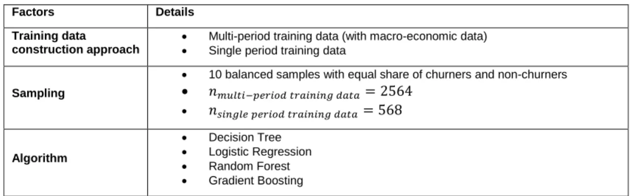
Table 4: Factors to build competing models ... 45

Table 5: Sampling the training data sets ... 46

Table 6: Top 10 churn predictors from ensemble methods and R square variable selection .. 57

Table 7: Maximum likelihood analysis result of a logistic regression model on multi-period training data ... 58

(8)

1 Introduction

1.1 Background

Churn classification is the important first step in customer retention

Customer retention has been the focus of customer relationship management research in the financial sector over the past decades (Zoric, 2016; Gur Ali & Ariturk, 2014; Koh & Chan, 2002, Reichheld & Kenny, 1990). Retaining existing customers is argued to be more economical over the long run for companies than acquiring new ones (Gur Ali & Ariturk, 2014). Van den Poel & Lariviere (2004), in their attempt to translate the benefits of retaining customers over a period of 25 years into monetary terms, concludes that an additional

percentage point in customer retention rate contributes to an increase in revenue of

approximately 7% (Van den Poel & Lariviere, 2004). Moreover, in their later search, Van den Poel & Lariviere (2005) indicates that acquiring new customers rather than retaining existing ones is not only costlier but also riskier because customers who have earlier switched among different service or product providers are more likely to do so again. Specifically in banking, affluent customers holding different types of assets are usually more skillful in diversifying their portfolios among various financial institutions and hence more difficult to retain than customers with fewer assets (Lariviere & Van den Poel, 2005). As a result, maintaining long term relationships with customers has been the common strategy among leading companies in the financial industry (Nie, et al., 2011), especially in retail banking (A. O. Oyeniyi & A.B. Adeyemo, 2015).

A recent survey conducted by Accenture indicates that retail banking customers worldwide are more knowledgeable to proactively purchase their banking services not only from banks but also from non-traditional service providers, such as fin-tech start-ups

(Accenture, 2015). As a result, customer retention has become a strategic priority because the longer the customers stay loyal to the banks, the more likely they are to expand their portfolio with the banks’ in-house services and the higher their customer lifetime values become (Reichheld & Kenny, 1990). Due to regulatory requirements, banks must store a vast amount of historical data of customer transactions and interactions, enabling substantial research on customer retention for retail banking customers (A. O. Oyeniyi & A.B. Adeyemo, 2015).

(9)

Introduction 1. The first step involves building a model to identify the so-called churn events,

which refer to the behavior of customers to switch from the current service or product provider to a competitor. The term “churn” is widely adopted in customer retention literature. The terms “churn classification” and “churn prediction” are used to refer to the first step of customer retention, which is to classify customers into binary groups: churners and non-churners. In this context, “churners” refer to the customers that are highly likely to switch to a competitor service or product provider and “non-churners” are the customers who are more loyal to their current services or products. Therefore, the result of the first step in customer retention is the creation of a churn classification model.

2. The second step of customer retention is to determine the customers who are worth retaining the most among the classified churners and take actions to incentivize the continuation of their relationship with the organizations (Ballings & Van den Poel, 2012).

Consequently, in order to achieve a high customer retention rate, being able to predict churn using a good churn classification model plays a vital role (van Wezel & Potharst, 2007). This thesis focuses on the first step of customer retention. A churn classification model trains an algorithm on a specific training data set to classify the observations into binary groups: churners or non-churners. A training data set is a matrix that consists of multiple rows and columns, where observations are presented as rows and the features of each observation, also known as independent variables or predictors, are presented as columns. A churn algorithm is also called a binary classifier in other studies (Gur Ali & Ariturk, 2014; Breiman, 2001) because the dependent variable of the churn classification model can take only binary values: 1 for churners or churn events and 0 or -1 for non-churners or non-churn events depending on the notation of the churn algorithms. Dependent variables in churn classification context can be called churn responses or target variables. Also, churn events and non-churn events are generally called positive and negative events in churn prediction problems. All the mentioned alternative terms are used interchangeably throughout this thesis.

The rarity issue of churn events in churn classification problems

The main characteristic, and also challenge, of churn classification studies is that churn is usually a rare event. Churn rate depends on the research domains and how churn is defined.

(10)

2014) while churn rate in retail banking context is usually less than 1% (Gur Ali & Ariturk, 2014). This rarity feature makes churn classification difficult for several reasons. First of all, churn is rare both in the number of churners and in proportion to the number of non-churners. These features of absolute rarity and relative rarity (Weiss, 2004) hinder the ability of churn classifiers to predict the churners accurately because the training data is overwhelmed with the majority of non-churners (Lemmens & Croux, 2006). Additionally, in the research conducted by Weiss (2004) on the challenges that frequently manifest in data mining techniques due to the rarity issue, he has criticized that some common metrics for model performance evaluation do not take this rarity characteristic into account; for example churn events have less impact on model accuracy than non-churn events due to their disproportional frequencies, therefore model accuracy should not be considered as an effective criteria for churn model comparison. Moreover, data mining algorithms that partition data into smaller pieces such as decision tree suffers from data fragmentation because the more leaves there are in the tree, the less churn events there are in each leaf. Such partitioning rule decreases the ability of the model to learn about the churn behavior and to generalize on data sets different from the training data (Weiss, 2004). In order to address this rarity issue, Weiss (2004) discusses some of the most widely used solutions in data mining like more appropriate evaluation metrics, various sampling methods like under-sampling of the majority non-churn events or over-sampling of minority events, cost-sensitive learning, or boosting algorithm in ensemble methods (Weiss, 2004).

Multi-period training data and ensemble methods have emerged in churn classification studies to overcome the rarity challenge

Over the past years, churn classification literature has evolved to incorporate some of the above mentioned solutions to improve the two main aspects of a churn classification model: the training data and the algorithm (Ballings & Van den Poel, 2012). Regarding the training data, much focus has been drawn to the enhancement of the training data for churn classification models from different angles; most notable are the three followed points:

1. More diverse data sources for churn predictors, or independent variables (Baecke & Van den Poel, 2009)

Churn classification models are argued to perform better with churn predictors from more diverse data sources in addition to internally collected data from the organization. Predictors such as macro-economic factors (Gur Ali & Ariturk, 2014; Mavri & Ioannou,

(11)

Introduction 2008) or commercially available data from external vendors (Baecke & Van den Poel, 2009) have been included in churn classification models to capture unseen factors from the macro-environment that might affect churn behavior. Such approach has shown to improve churn model performance compared to the churn predictors merely aggregated from customer transactions (Gur Ali & Ariturk, 2014; Baecke & Van den Poel, 2009; Mavri & Ioannou, 2008).

2. Inclusion of longitudinal data for churn responses (Gur Ali & Ariturk, 2014) The inclusion of longitudinal data of churn response is claimed to improve churn classification performance with statistical techniques such as survival analysis but has not received much attention in churn classification algorithms (Gur Ali & Ariturk, 2014). Gur Ali & Ariturk (2014) stresses the importance of time series data in enabling early detection of churners, providing an opportunity for marketers to act timely in their customer retention campaigns. Churn literature traditionally employs churn responses calculated at the most recent point of time, hence information about customers that have churned prior to the pre-defined churn period is discarded and the variation of churn probability over time due to other aspects such as macro-economic factors is ignored. Moreover, independent time series variables are usually aggregated into static values such as min, max or average over the observation period. Such approach is argued to possibly rid the model of important

information from the time series nature of the transactional data (Gur Ali & Ariturk, 2014). 3. Appropriate time window of analysis (Ballings & Van den Poel, 2012)

The time window of analysis is also studied to increase model efficiency. Time window of analysis refers mainly to the two periods of time: observational period, used to capture the independent variables, or churn predictors and performance period, used to calculate the dependent variables, or churn responses. Ballings & Van den Poel (2012) focuses on the former time window for the independent variables, which are mainly comprised of

transactional data over time in churn classification context, to optimize the duration of such period. In their response to the natural question “How long back in time should the data be included to build the best performing model?”, Ballings & Van den Poel (2012) rejects the common belief that performance improves proportionally with the increasing data volume because it is observed in their research that over the time window of 77 years, after a specific point of time say 15 or 16 years, one additional year of historical data does not solve the lack of churn data issue but only creates computational burden (Ballings & Van den Poel, 2012).

(12)

Furthermore, Gur Ali & Ariturk (2014) evaluates models that includes the lagged values for all independent variables and observes that such models perform worse than those without the lagged variables (Gur Ali & Ariturk, 2014).

Taking into consideration all the three aforementioned aspects, Gur Ali & Ariturk (2014) proposes the multi-period training data approach, in which both churn responses and churn predictors are captured over multiple periods of time. As such, one customer can have many observations over time and historical information about churn responses prior to the defined churn period is retained as much as the operational data allows; therefore, the models are claimed to make more effective use of the historical churn responses rather than throwing them away, mitigating the rarity issue. In their studies, models that employ this approach to construct the training data are compared with models that employ the so-called single period training data approach. Single period training data refers to the traditional approach, in which both churn responses or dependent variables and churn predictors or independent variables are captured only at a single point of time. Specifically, the churn responses are calculated from the most recent data while the values of the independent variables or churn predictors are aggregated over a period of time prior to the churn period. In a study to predict churn among private customers in a commercial bank, for both models that employ logistic regression and decision tree as churn classification algorithms, the multi-period training data approach is concluded to outperform the single period training data approach (Gur Ali & Ariturk, 2014). However, the proposed multi-period training data approach has been applied to only a few churn classification algorithms such as decision tree or logistic regression. Consequently, there is a need to investigate whether the proposed multi-period training data also performs well in churn classification models using other algorithms.

Regarding churn classification algorithms, researches have recently developed a wide variety of classification algorithms that perform better than logistic regression and decision tree to predict churn. It is worth mentioning that over the history of churn prediction,

different techniques have been employed, such as segmentation based on recency, frequency and monetary (usually denoted as RFM) information from customer transactional data; statistical techniques such as logistic regression and survival analysis (Mavri & Ioannou, 2008; Van den Poel & Lariviere, 2004); data mining techniques for large data set such as decision trees (Nie, et al., 2011; van Wezel & Potharst, 2007); and more advanced machine learning techniques like neural networks and support vector machine (Baecke & Van den Poel, 2009). Not until recently has churn prediction literature discovered the superiority of

(13)

Introduction ensemble method in churn classification compared to logistic regression and decision tree. Ensemble method generally refers to the combination of two or more models into a single and more powerful one (Yaya, et al., 2009; Jinbo, et al., 2007; Lariviere & Van den Poel, 2005). In some studies that employ ensemble methods, the algorithms used in churn classification are also called churn classifiers (Breiman, 2001). This term will be used throughout the thesis interchangeably with churn algorithms. Among the employed ensemble methods in churn classification, random forest and gradient boosting have been concluded to outperform logistic regression and decision tree in several researches (Van den Poel & Lariviere, 2005 & 2004; Breiman, 2001). Therefore, the thesis considers these two methods from the ensemble family good candidate for the comparative study in the housing loan context.

As a result, this thesis aims to investigate whether the proposed multi-period training data by Gur Ali & Ariturk (2014) improves churn classification accuracy for models that use ensemble methods, namely random forest and gradient boosting, compared to those using logistic regression and decision tree. Moreover, to the best of the author’s knowledge, this multi-period training data approach has not been employed in any other researches. In that manner, the thesis is an extension to the research by Gur Ali & Ariturk (2014) by applying their proposed multi-period training data approach to more complexed churn algorithms to examine whether the performance of this approach stays robust in the domain of housing loan churn.

1.2 Research Problem and Contribution

In light of the background on churn classification, this thesis focuses on the first step of customer retention, which is to build a churn classification model with the consideration of the proposed ideas to improve the training data and the advanced algorithms: specifically, the multi-period training data proposed by Gur Ali & Ariturk (2014) and the ensemble methods as advanced churn classifiers. The thesis has acknowledged a gap in the application of the proposed multi-period training data approach by in churn classification; the author aims to test the robustness of this approach with ensemble methods, namely random forest and gradient boosting, in the context of housing loan churn prediction. Specifically, the thesis first validates whether the multi-period training data approach performs better than the traditional single period training data approach using logistic regression and decision tree as churn classification algorithms. Secondly, the thesis incorporates this multi-period training

(14)

data approach and the advanced ensemble methods in churn classification models and examines their performance in churn classification.

This thesis aims to explore the research problem in churn prediction of housing loan customers in the retail banking segment of a Nordic bank. Despite the large volume of churn prediction studies in retail banking, most of them concentrate on churn in general (Zoric, 2016; Prasad & Madhavi, 2012; Van den Poel & Lariviere, 2004) or in credit card segment (A. O. Oyeniyi & A.B. Adeyemo, 2015; Nie, et al., 2011). Only little research focuses particularly on housing loan customer (Koh & Chan, 2002); therefore, this research also enriches churn literature for this customer segment.

The research problem is detailed into the following research questions. Based on the selected evaluation criteria,

Question 1: For models that employ logistic regression and decision tree, does multi-period training data approach improve churn classification performance than the single period training data approach?

Question 2: For models that employ single period training data, do random forest and gradient boosting improve churn classification performance than logistic regression and decision tree?

Question 3: Do models that employ both multi-period training data approach and ensemble methods perform better in churn classification than those in the first

question?

Question 4: What are the best churn predictors in the housing loan context? The first two questions aim to validate whether the multi-period training data approach and the ensemble methods perform better in churn classification for the housing loan

customers compared to their counterparts. The third question studies whether their

combination improves the churn classification performance even further. If the result in this thesis supports the hypothesis that models, which employ the multi-period training data approach and random forest and gradient boosting as churn classifiers, perform better than the other models created in the thesis, it is sensible to expand the application of this multi-period training data approach proposed by Gur Ali & Ariturk (2014) in churn classification. Finally, the last question is of general managerial interest when it comes to churn prediction to highlight the best churn predictors.

(15)

Introduction

1.3 Research Structure

The structure of this thesis is illustrated by Figure 1. Chapter 2 provides an extensive literature review on the selected aspects of churn classification modelling. Chapter 3 reviews the employed research methodologies in this thesis. Chapter 4 describes the data by

explaining the procedure to calculate the churn responses for the housing loan customers of the case company, the time windows of analysis, and the preparation of the churn predictors or independent variables. Chapter 5 discusses the model building process and the models’ results. Chapter 6 concludes the thesis with its contribution, limitations and suggestions for future research in the churn classification topic.

Figure 1: Thesis structure

Chapter 1: Introduction

•Multi-Period Training Data

•Churn Classification Algorithms

•Churn Predictors

•Evaluation Criteria

Chapter 2: Literature Review

•Logistic Regression

•Decision Tree

•Bagging and Boosting

•Random Forest

•Gradient Boosting

Chapter 3: Research Methodology

•Calculating Churn Responses - Dependent Variable

•Time Window of Analysis

•Preparing the Independent Variables Chapter 4: Data

•Building Competing Models

•Answering the research questions Chapter 5: Results

(16)

2 Literature Review on Churn Prediction

This chapter reviews the selected aspects of churn classification modelling. First, the author describes the proposed multi-period training data approach proposed by Gur Ali & Ariturk (2014). Second, the thesis discusses the most widely used churn algorithms and argues for the selected ensemble methods for this thesis. Then, the thesis reviews the main groups of churn predictors that have been used in churn classification literature. This section concludes with the evaluation criteria that are commonly used to assess churn model performance and are employed in this thesis.

An overview of these aspects in churn literature over the past years is summarized in Table 1. The details are discussed in the sub-sections below.

(17)

Literature Review on Churn Prediction

Table 1: An overview of several recent churn studies

Reference

Churn problem context

Churn predictor Training data construction

Churn algorithms and their

performance Evaluation criteria

Demogra phic Customer behavior Relationship characteristic External data Time-varying churn predictors Time-varying churn responses

(Fitzpatrick & Mues, 2015) Banking x x

Boosted Regression Trees, Random forests, Generalized Additive Models > Logistic Regression

H measure, Area Under Curve (ROC Index)

(Gur Ali & Ariturk, 2014) Banking x x x x x x

Binary classification > Survival analysis (Multi-period period) Logistic Regression > Decision Tree (Single period prediction)

Area Under Curve (ROC Index), Top Decile Lift (Lemmens & Gupta, 2013) Telecom. x x x

Stochastic Gradient Boosting with profit loss function > Logistic Regression or Decision Tree

Gain/loss matrix (Ballings & Van den Poel,

2012) Media x x x x

Bagging of classification trees > Logistic Regression > Decision Tree

Area Under Curve (ROC Index) (Lee, et al., 2012) Telecom. x x x x k-nearest-neighbor time series

classification

N/A (Nie, et al., 2011) Banking x x x Logistic Regression > Decision

Tree

Type I Type II error, misclassification cost

(Yaya, et al., 2009) Banking x x

Improved Balanced Random forests > Support Vector Machine > Neural Network > Decision Tree

Lift curve, Top Decile Lift (Burez & Van den Poel, 2009)

Banking, Telecom., Media, Retail

- - - Random forests > Logistic _Regression

Area Under Curve (ROC Index), Lift (Qi, et al., 2008) Telecom. x x x x

ADTreeLogit > ADTree (Alternative Decision Tree) > Logistic regression

Area Under Curve (ROC Index) (Mavri & Ioannou, 2008) Banking x x x x x Survival analysis (Cox

regression)

(18)

(van Wezel & Potharst, 2007) Retail x x x Multi-boosted CART > Boosted CART > CART

Error rate (Lemmens & Croux, 2006) Telecom. x x x

Stochastic Gradient Boosting > Bagging of Decision Tree > Binary Logit Model

Error rate, Top Decile Lift, Gini Coefficient (Lariviere & Van den Poel,

2005)

Financial

service x x x

Random forests > Logistic Regression

Area Under Curve (ROC Index)

“-“ = not mentioned “blank” = not used

(19)

2.1 Multi-period Training Data

As can be seen from Table 1, under the header “Training data construction”, time-varying churn predictors are employed fairly often among recent research whereas very few studies include time-varying churn responses in their training data. Such an observation confirms the argument by Gur Ali & Ariturk (2014) that even though the inclusion of time series data for both churn predictors and churn responses has been found to increase churn classification accuracy, the approach has not been employed much. The thesis now discusses the proposed multi-period training data approach by Gur Ali & Ariturk (2014), which has been found to outperform the traditional approach, which is called single period training data by Gur Ali & Ariturk (2014) in their research.

First, it is worth starting the discussion with the single period training data approach that captures only one churn response for each customer at a specific point of time. In other words, one customer constitutes only one row in the training data set. Meanwhile, the time-varying predictors are summarized over the most recent period of time into single columns instead of time series using simple aggregation. Examples of such independent variables in some churn prediction studies are average of monthly minutes of use over the past six months, the percentage change compared to the previous six months in a telecommunication churn study (Lemmens & Croux, 2006), or total credit or debit transactions in the last three months in a retail banking churn study (Prasad & Madhavi, 2012). The term “single period training data” is used to refer to such an approach, which is illustrated as below:

𝑆𝑃𝑇𝐷_𝑡 = [𝑌_𝑡 𝑆 𝐷_𝑡−𝛿]

• 𝑆𝑃𝑇𝐷_𝑡 is the single period training data for the churn period 𝑡

• 𝑌_𝑡 is a vector or an 𝑛 x 1 matrix of churn responses 𝑦 at time 𝑡 of 𝑛 customers

• 𝑆 is an 𝑛 x 𝑠 matrix of non-time varying variables 𝑠𝑖𝑗 for 𝑛 customers. The most

popular variables employed in churn prediction that are not changing over time are usually demographic variables like gender or, within the time window of a year, age and educational level.

• 𝐷𝑡−𝛿 is an 𝑛 x 𝑑 matrix of time varying variables 𝑑𝑖𝑗 for 𝑛 customers at time 𝑡 − 𝛿, where 𝛿 is the length of either the operational lead time for data to be available in the internal databases or of the lead time reserved for customer

(20)

retention action between the observation period and the time when churn behavior is supposed to occur.

Figure 2 illustrates a general time window of analysis in traditional churn prediction studies: the observation period provides the training data for the model, the performance period is the time when churn is defined, and the interval between these two periods is allowed for marketing action to retain worth-while customers (Lu, et al., 2014).

Figure 2: Time window of analysis illustration for single period training data

In order to capture the time variation in both churn predictors and churn response, the multi-period training data is composed of multiple single period training data sets ranging from the latest possible point of time 𝑡 back in time to get the historical churn responses. Such point of time is denoted as 𝑘 in the below formula for the multi-period training data:

𝑀𝑃𝑇𝐷_𝑡 = [ 𝑆𝑃𝑇𝐷_𝑡 𝑆𝑃𝑇𝐷_𝑡−1 ⋮ 𝑆𝑃𝑇𝐷_𝑘+1 𝑆𝑃𝑇𝐷_𝑘 𝐸 ] = [ 𝑌_𝑡 𝑆 𝑌_𝑡−1 ⋮ 𝑌_𝑘+1 𝑆 ⋮ 𝑆 𝑌_𝑘 𝑆 𝐷_𝑡−𝛿 𝐸_𝑡−𝛿 𝐷_{𝑡−1−𝛿} ⋮ 𝐷_{𝑘+1−𝛿} 𝐸_{𝑡−1−𝛿} ⋮ 𝐸_{𝑘+1−𝛿} 𝐷_𝑘−𝛿 𝐸_𝑘−𝛿 ] • 𝑀𝑃𝑇𝐷𝑡 is the multi-period training data for the churn period 𝑡

• 𝑆𝑃𝑇𝐷_𝑡 is a matrix of single period training data as shown below, illustrating that the multi-period training data is comprised of multiple single period training data matrices. Although it is more probable that the single period training data sets have various numbers of observations in practice, for the sake of simplicity in mathematical illustration, the single period training data sets are assumed to have equally 𝑛 observations.

• 𝐸 is a 𝑛(𝑡 − 𝑘) x 𝑒 matrix of time-varying macro-environmental factors 𝑒_𝑖𝑗

during the specified period. As can be seen in single period training data and multi-period training data formulas, it is not possible to include environmental predictors in single period training data because only one point of time is included (Gur Ali & Ariturk, 2014).

(21)

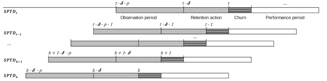
Figure 3: Time windows of analysis illustration for single period training data and multi-period training data

• 𝒕 is the time when the latest churn response is recorded over a pre-defined period of time. The churn period of the housing loan data in this thesis is one month.

• 𝜹 is the length of the period reserved for marketing retention action; hence the starting point of this period is 𝒕 − 𝜹. For this thesis, 𝜹 is assumed to be one month.

• 𝒌 is the time when the earliest churn response is recorded.

• 𝒑is the length of the observation period, when the time series of input variables are aggregated.

• After each churn period, the performance period starts to capture the post-churn criteria for churn response calculation.

Each of the periods is marked and labelled accordingly in each single period training data set. The lengths of these periods can always be adjusted accordingly to fit the business context.

… t t + 1 … t + s Churn t - 1 … t - 1 … t - 1 Performance period

Observation period Retention action

_𝒕− _𝒌 _𝒌+ _𝒕 t t -t - - p t - 1 t - - 1 t - - p - 1 k + 1 k + 1 -k + 1- - p k k - - p k

(22)

-An illustration of the time windows of analysis for single period training data and multi-period training data is provided in Figure 3.

Multi-period training data includes multiple periods of single period training data from time 𝑡, when the latest churn response is recorded, backwards to time 𝑘 to obtain the

historical churn responses. The factors to determine 𝑘 include the availability of data, the tenure of the customers and the computational efficiency of the model. If the single period training data sets are assumed to have equally 𝑛 observations, then the multi-period training data has 𝑛 ∗ (𝑡 − 𝑘) observations. This obvious increase in the data size might create

computation burden for the model; hence it might not be always a good idea to include all the historical data available.

The additional observations are not generated from the current data set as in different sampling schemes (Burez & Van den Poel, 2009) but are taken from the otherwise discarded data from historical behaviors and churn responses; hence, one customer can have as many observations as the periods of time that they are active. As a result, the models are fed with considerably more new data than in the single period training data approach, a characteristic that is claimed to boost the learning capacity of churn models. Most importantly, even though the churn ratio is the same in both training sets, the multi-period training data has

theoretically (𝑡 − 𝑘) times more churners than the single period training data in absolute number assuming the churn rate remains constant over the period of time, mitigating the absolute rarity problem, which is the main purpose of the proposed approach. Finally, multi-period training data does not suffer from the curse of dimensionality with the large additional data amount because these data are added as rows in the training data set instead of columns. Curse of dimensionality generally refers to the phenomenon that when the sample data size does not increase exponentially in response to the increase in the number of variables, the data becomes sparse in this high dimensional space, causing problems to the models, such as overfitting the data to the model, especially in churn problems when churn events are rare. (Gur Ali & Ariturk, 2014)

The last point is illustrated by constructing also a single period training data + lags training data as shown in the equation below:

𝑆𝑃𝑇𝐷 + 𝑙𝑎𝑔𝑠_𝑤 =[𝑆𝑃𝑇𝐷_𝑡 𝐷_{𝑡−𝛿−1} 𝐷_{𝑡−𝛿−2} … 𝐷_{𝑡−𝛿−𝑤−1}] = [𝑌𝑡 𝑆 𝐷𝑡−𝛿 𝐷𝑡−𝛿−2 … 𝐷𝑡−𝛿−𝑤−1]

(23)

Literature Review on Churn Prediction 𝑆𝑃𝑇𝐷 + 𝑙𝑎𝑔𝑠 includes single period training data plus the predictors’ values during the time between the 𝑡 and the lags 𝑡 − 𝑤; consequently, for each independent variable there are

𝑤 more columns or dimensions in the training data while the total sample size is the same as the single period training data. Among the three approaches, models built from single period training data + lags perform the worst because, among other things, it suffers from the curse of dimensionality explained above.

However, multi-period training data is not without its own limitations. Figure 3 shows that the observation periods for the single period training data sets within multi-period

training data are highly overlapping for two consecutive periods. Consequently, the data used to aggregate the time varying variables 𝑑𝑖𝑗 for the same customers are largely overlapping,

and the resulting time-varying predictors are highly correlated. This phenomenon is called multi-collinearity in statistical models, when independent variables in a model are highly correlated with one another, hindering the reliability of the estimated parameters (Van den Poel & Lariviere, 2004). Moreover, time series are prone to be highly correlated with their lagged values, worsen the multi-collinearity among the time-varying variables for the same customers. It can be said that employing longitudinal data from the same customers do not conform to the rule of independent and identical distribution; and such characteristic might bias the estimated parameters in statistic algorithms such as logistic regression (Gur Ali & Ariturk, 2014). In response to these limitations, Gur Ali & Ariturk (2014) emphasizes the goal to improve the performance of binary classification models instead of correcting biased parameters. Their study shows that multi-period training data outperforms the other two approaches single period training data and single period training data + lags in churn

prediction for both next period and multiple periods (Gur Ali & Ariturk, 2014). Additionally, as single period training data + lags approach consistently produces the worse performances among the three proposed.

2.2 Churn Classification Algorithms

As can be seen from Table 1, under the column “Churn algorithm and their

performance”, logistic regression and decision tree are employed in nearly all of the reviewed papers, especially when comparison with other more advanced algorithms is needed. This section discusses the churn algorithms that have been used in churn classification and argues for the selected ones to employ in this thesis.

(24)

Logistic regression is a statistical method that returns a probability for each observation as the output variable; as a result, it is frequently chosen as the scoring method for the

probability to churn among customers. At a specific cut-off (usually 0.5), customers with the estimated probabilities higher than the cut-off point are marked as predicted churners and the rest are predicted non-churners. Logistic regression is frequently chosen in marketing

research that deals with individual customers because the model presents the assumed relationship between the independent variables and the dependent variable descriptively, making it possible to interpret how significant and how much an independent variable is able to explain the target variable based on the estimated parameters. Moreover, logistic

regression has been found to perform relatively well compared to other more complex models with various data sets from different domains (Fitzpatrick & Mues, 2015). Thanks to its robustness, logistic regression is used a great deal in churn prediction, especially as the baseline in comparison studies (Fitzpatrick & Mues, 2015; Gur Ali & Ariturk, 2014; Lemmens & Gupta, 2013; Ballings & Van den Poel, 2012).

The other popular algorithm in marketing generally and churn classification specifically is decision tree thanks to its clear presentation in the tree structure to show the most

significant rules that define the target variable; hence, decision tree has been employed in churn prediction with the ambition to capture the rules from customer behaviors that can detect early signs of churn (Gur Ali & Ariturk, 2014; Lemmens & Gupta, 2013; Nie, et al., 2011). However, decision tree models are usually associated with lack of robustness and sub-optimal performance in churn literature (Lariviere & Van den Poel, 2005). As a result, it can be observed from Table 1 that a wide range of complex models have been developed based on decision trees such as Multi-boosted CART, Boosted CART (Qi, et al., 2008), ADTree (van Wezel & Potharst, 2007), bagging and boosting of classification tree (Ballings & Van den Poel, 2012; Lemmens & Croux, 2006), stochastic gradient boosting (Lemmens & Gupta, 2013), or random forests (Van den Poel & Lariviere, 2005 & 2004). Additionally, more complicated models can be developed not only from decision tree but also from its combination with logistic regression algorithm like ADTreeLogit (Qi, et al., 2008).

Most of the advanced algorithms listed above belong to the ensemble family, revealing the wide application of ensemble methods in churn prediction. In general, ensemble refers to the different methods to combine two or more models into a single yet more powerful one with the aim to improve predictive performance (Yaya, et al., 2009; Jinbo, et al., 2007; Lariviere & Van den Poel, 2005). The most widely used methods in ensemble modelling are

(25)

Literature Review on Churn Prediction bagging and boosting. Both methods use an algorithm as a base learner to train a model repeatedly on different samples of the original data; finally for each observation, a single predictive score is aggregated from the iterative training. In this case, a base learner is

basically an algorithm that is selected to be trained iteratively to produce an ensemble model. The typical base learner in churn classification is decision tree (Chrzanowska, et al., 2009; Qi, et al., 2008; Lariviere & Van den Poel, 2005). A brief review on bagging and boosting is provided in the section 3.3.3 under Research Methodology.

The most powerful and frequently used bagging method in churn prediction is random forest (Yaya, et al., 2009; Lariviere & Van den Poel, 2005; Chen, et al., 2004). Random forest has been found to provide better estimations for binary classification of customer churn than ordinary linear regression and logistic regression (Lariviere & Van den Poel, 2005). In order to improve the capability of churn prediction models in handling imbalanced data, various enhanced versions of random forest models incorporate sampling techniques and cost optimization training. In the research conducted by Chen et al. (2004), the improved versions of random forests are trained on 6 different data sets in various domains from oil exploration to Hypothyroid and Euthyroid diagnoses to produce better churn classification results

compared to other existing techniques like logistic regression and decision tree (Chen, et al., 2004). In another research, Yaya, et al. (2009) combines all the improvements suggested by Chen, et al. (2004) into one model called improved balanced random forest, which reveals to provide more accurate churn prediction compared with neural network and decision tree models (Yaya, et al., 2009).

On the other hand, the boosting algorithms popularly employed in churn prediction are stochastic gradient boosting (Lemmens & Gupta, 2013) and AdaBoost (Lu, et al., 2014; Jinbo, et al., 2007). Although stochastic gradient boosting is claimed to be the most

sophisticated algorithm in the boosting family, it has been found to outperform binary logit model while performing comparatively with bagging in a churn prediction study of the telecommunications industry (Lemmens & Croux, 2006). In a more recent research,

stochastic gradient boosting has been employed in junction with a proposed loss function by Lemmens & Gupta (2013) and has been found to increase the profitability of retention campaigns compared to logistic regression for a telecommunications company (Lemmens & Gupta, 2013).

(26)

family. A technical reason for the selection is the possibility to run these models in SAS Enterprise Miner. In conclusion, four algorithms are employed in this thesis to build churn prediction models: logistic regression and decision tree as the standard algorithms, random forest and gradient boosting as the candidates for the advanced methods.

2.3 Churn Predictors

The most widely used churn predictors can be categorized into the following groups: demographic data, customer behavior data, customer satisfaction data, and external factors (A. O. Oyeniyi & A.B. Adeyemo, 2015; Nie, et al., 2011; Van den Poel & Lariviere, 2004; Koh & Chan, 2002).

First of all, demographic data such as gender, age, salary, or educational level are static variables that are usually assumed to remain unchanged over the time window of analysis within a year (Gur Ali & Ariturk, 2014; Mavri & Ioannou, 2008; Koh & Chan, 2002). For example, age and gender are found to be significant to predict churn behavior among banking customers (Koh & Chan, 2002). In another study of customer switching behavior for a Greek bank using survival analysis, Mavri & Ioannou (2008) finds that the age group 30 – 40 years old is the most likely to evaluate their cooperation with the existing bank and seek for better terms elsewhere (Mavri & Ioannou, 2008). However, it is often a challenge for banks to obtain high quality for demographic data due to the fact that customers are not mandated to provide all the information in this category. For example, customers do not have to provide their educational level or monthly salary if they do not purchase products that requires such information (Employee, 2016). Therefore, these demographic variables have a high level of missing data and hence, frequently dismissed from the models (Prasad & Madhavi, 2012). Additional to age and salary, lifecycle stage is also employed in churn prediction in the banking context as it is found to significantly impact how customers prioritize their financial differently at different life stages, for example young customers have less money to spend, hence have smaller investment portfolios than their more mature counterparts (Lariviere & Van den Poel, 2005).

Second, customer behavior from transactional databases has been deemed the most important group of predictors for churn literature because of the recency, frequency and monetary (RFM) information that they provide (Ballings & Van den Poel, 2012; Baecke & Van den Poel, 2009). This group of churn predictors also includes information about product

(27)

Literature Review on Churn Prediction portfolio in terms of volume and their changes over time (Lariviere & Van den Poel, 2005 & 2004).

The third group of churn predictors is the characteristic of customer relationship with the organization, for example, customer interaction with the bank in terms of contacts and tenure (Gur Ali & Ariturk, 2014; Ballings & Van den Poel, 2012; Mavri & Ioannou, 2008). Additionally, customer satisfaction’s impact on churn behavior in the banking context has also been studied extensively. Findings suggest that customer satisfaction and customer’s perception towards the company’s image have a great influence on customer loyalty and the duration of customer relationship. Using proportional hazard method to compare the

influence of various predictors on churn behavior, Mavri & Ioannou (2008) discovers that there is a significant difference in churn probability between customers that rank the bank’s service as “very important” and “extremely important” (Mavri & Ioannou, 2008). An

interesting suggestion from Lariviere & Van den Poel (2005) is the employment of variables related to intermediaries, or particularly sales agents. Examples of such variables are the extent to which the salesperson is prone to cross-sell, the product variety in the offerings from a salesperson, and the number of customers served by a salesperson. In their churn model using random forests, these variables, especially the tendency to sell of the sales person are found to significantly impact customers’ decision either in both cross-buying and churn contexts (Lariviere & Van den Poel, 2005).

Last but not least, the fourth group of churn predictors employed in the literature is the external information extracted outside companies’ internal data. In dynamic churn literature, churn behavior is argued to be affected by the changing economic conditions that are unseen from the companies’ internal databases. Therefore, models, where churn response and independent variables are limited to only a specific time period, cannot employ these time-varying environmental predictors and hence, cannot capture the dynamic variation in churn behavior (Gur Ali & Ariturk, 2014). In their dynamic churn prediction research for private banking customers, Gur Ali & Ariturk (2014) confirms the relevance of macro-economic variables in explaining churn responses. For example, deposit interest rate has a significant effect on private customers’ decision to switch banks because most of the private customers’ assets are fixed rate deposits (Gur Ali & Ariturk, 2014). Ballings & Van den Poel (2012) also includes a predictor that captures the historical merger and acquisition situation of a financial organization when studying its customers’ churn behavior over the period of 77 years. This

(28)

finding that aligns with the market perception about the merger (Ballings & Van den Poel, 2012). Fitzpatrick & Mues (2015) also specifies the hidden non-linear relationship between the churn response and the unseen variables that might be external to the company’s context such as unemployment rate in a specific region (Fitzpatrick & Mues, 2015). When comparing with behavior predictors, customer satisfaction and macro-environmental factors are found to have more significant impact on churn behavior (Mavri & Ioannou, 2008).

Baecke & Van den Poel (2009) points out two major limitations of internal data that banks are passively collecting from their customers’ information and behavior. First of all, these internal databases represent the limited versions of customers that are observed by the banks. For example, the data only tells what products and by how much a particular customer has purchased but provides no inference about the over-all needs for the total product

category. He/she might be purchasing a similar product from a competitor at the same time. However, such data is not available for banks internally. Additionally, focusing on

transactional data does not provide banks with an understanding of the motivation and

attitudes that drive these purchases. This drawback is argued to possibly hinder the possibility to build long term relationship with customers (Baecke & Van den Poel, 2009). Lariviere & Van den Poel (2005) also advocates the use of geo-demographic data from external data sources to build a more comprehensive picture of the customers (Lariviere & Van den Poel, 2005)

In conclusion, the richer of information that the training data includes, the better the model performs. Nie et al. (2011) compares the performance to predict churn in credit card customers by building multiple models using both single source of information and

combination of different sources such as customer demographic data, cards general information, transaction information and risk related information. The model built from a diverse independent variable set outperforms the ones with less diverse data (Nie, et al., 2011). To the author’s best knowledge, such approach has not been done for churn problem in the banking context, however, the conclusion is argued to remain that the more diverse the data is, the better the model performs.

2.4 Evaluation Criteria

Even though churn literature employs a wide selection of algorithms, as can be seen from Table 1, only a few criteria for performance evaluation are universally selected for model comparison such as misclassification rate, AUC (Area under Curve) or ROC (Receiver

(29)

Literature Review on Churn Prediction Operating Characteristic) index, and top decile lift (Gur Ali & Ariturk, 2014; Nie, et al., 2011; Yaya, et al., 2009; Burez & Van den Poel, 2009; Lemmens & Croux, 2006). These evaluation metrics and some of their improved forms are argued to take into consideration the imbalanced data set in churn problem (Weiss, 2004).

The next sub-sections provide more detailed reviews on the selected evaluation criteria in this thesis: misclassification rate, ROC index and top decile lift.

2.4.1 Misclassification Rate

Binary classification models do not naturally have 100% correct prediction but normally some of the real churners are misclassified as non-churners and vice versa, some of the real non-churners are misclassified as churners. Such statistics are shown in the confusion matrix in Table 2, where churn events are commonly denoted as positive events and non-churn events as negative events. As can be seen from the confusion matrix, among the predicted positive events, there are both true positive events and false positive events. The same applies to the predicted negative events, which include both false negative events and true negative events. True positive events refer to the real churners that are classified as churners by the model. Similarly, true negative events refer to the real churners that are classified as non-churners by the model. On the other hand, false positive events refer to the real non-non-churners that are misclassified as churners by the model while false negative events refer to the real churners that are misclassified as non-churners by the model.

Table 2: Confusion matrix of churn classification

Predicted Positive Predicted Negative

Real Positive True Positive False Negative

Real Negative False Positive True Negative

From these parameters in the confusion matrix, the accuracy is calculated as followed

𝐴𝑐𝑐𝑢𝑟𝑎𝑐𝑦 = 𝑛𝑢𝑚𝑏𝑒𝑟 𝑜𝑓 𝑐𝑜𝑟𝑟𝑒𝑐𝑡𝑙𝑦 𝑐𝑙𝑎𝑠𝑠𝑖𝑓𝑖𝑒𝑑 𝑒𝑣𝑒𝑛𝑡𝑠 𝑛𝑢𝑚𝑏𝑒𝑟 𝑜𝑓 𝑎𝑙𝑙 𝑒𝑣𝑒𝑛𝑡𝑠

and the misclassification rate is identified as followed

𝑀𝑖𝑠𝑐𝑙𝑎𝑠𝑠𝑖𝑓𝑖𝑐𝑎𝑡𝑖𝑜𝑛 𝑟𝑎𝑡𝑒 = 1 − 𝐴𝑐𝑐𝑢𝑟𝑎𝑐𝑦

(30)

Regarding the confusion matrix in Table 2, the false positive events and false negative events are also referred to as type I and type II errors in the binary classification literature. As a result, type I error refers to the number of the real non-churners that are misclassified as churners while type II error indicates the number of real churners that are misclassified as non-churners. A disadvantage of the misclassification rate is that it views the two types of error equally. Since the would-be churners that are not identified for the retention campaign will churn anyway, the bank will suffer a loss of future profits from the customers not only from housing loan products but also from other possible products that the customers might be or will be holding with the bank. On the other hand, non-churners that are misclassified as churners only cost the bank the unnecessary retention action because they will continue their relationship with the service provider anyway. Consequently, the loss caused by type II error for the company is argued to be much higher than type I error (Nie, et al., 2011). As a result, various loss functions have been designed to capture the actual loss of misclassification that is specific to each organization. Moreover, as it is more costly to falsely identify highly profitable customers than the less profitable ones, customer life time value has also been incorporated in loss functions to capture only the most worth-while customers to retain (Glady, et al., 2009; Lemmens & Croux, 2006). Additionally, Lemmens & Gupta (2013) looks at customer retention from the angle of profit maximization for the marketing campaign and incorporate both customers’ value and responsiveness to retention incentives in their loss function using stochastic gradient boosting to design the most profitable target size

(Lemmens & Gupta, 2013).

2.4.2 ROC Index

ROC stands for receiver operating characteristic (ROC) curve that assumes the form of a graph of (𝑥, 𝑦) where 𝑥 = 1 − 𝑠𝑝𝑒𝑐𝑖𝑓𝑖𝑐𝑖𝑡𝑦 𝑦 = 𝑠𝑒𝑛𝑠𝑖𝑡𝑖𝑣𝑖𝑡𝑦 𝑆𝑝𝑒𝑐𝑖𝑓𝑖𝑐𝑖𝑡𝑦 = 𝑛𝑢𝑚𝑏𝑒𝑟 𝑜𝑓𝑇𝑟𝑢𝑒 𝑁𝑒𝑔𝑎𝑡𝑖𝑣𝑒 𝑒𝑣𝑒𝑛𝑡𝑠 𝑛𝑢𝑚𝑏𝑒𝑟 𝑜𝑓 𝑅𝑒𝑎𝑙 𝑁𝑒𝑔𝑎𝑡𝑖𝑣𝑒 𝑒𝑣𝑒𝑛𝑡𝑠 and 𝑆𝑒𝑛𝑠𝑖𝑡𝑖𝑣𝑖𝑡𝑦 = 𝑛𝑢𝑚𝑏𝑒𝑟 𝑜𝑓 𝑇𝑟𝑢𝑒 𝑃𝑜𝑠𝑖𝑡𝑖𝑣𝑒 𝑒𝑣𝑒𝑛𝑡𝑠 𝑛𝑢𝑚𝑏𝑒𝑟 𝑜𝑓 𝑅𝑒𝑎𝑙 𝑃𝑜𝑠𝑖𝑡𝑖𝑣𝑒 𝑒𝑣𝑒𝑛𝑡𝑠

(31)

Literature Review on Churn Prediction For a binary classifier, the horizontal axis of a ROC curve shows the ratio between the number of falsely predicted positive events and the number of real negative events; while the vertical axis presents the ratio of the number of correctly predicted positive events out of the number of real positive events. As a result, the ROC curve plots the true positive rate (𝑦)

against the false positive rate (𝑥) (Gur Ali & Ariturk, 2014).

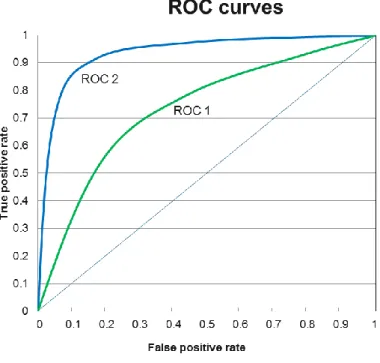
A few examples of ROC curves are demonstrated in Figure 4. The diagonal line connecting the points (0, 0) and (1, 1) represents the random guess that any customer is 50% a churner and a non-churner because on this line, the true positive rate is always equal to the false positive rate. Hence, the ROC curves that closely follow this diagonal line show the inability of the model to identify churn events against non-churn events. An ideal ROC curve is the one that follows closely the vertical axis at first with high true positive rate and low false positive rate and then curves closely towards the horizontal axis. Therefore, between the two lines denoted with ROC 1 and ROC 2 in Figure 4, the model with the ROC 2 curve is more preferable.

Figure 4: Example of a ROC chart

In order to provide the ROC index for model comparison, the area under the ROC curve, also usually referred to as the Area under Curve (AUC) in churn literature, is computed as shown by the formula below.

𝑅𝑂𝐶 𝑖𝑛𝑑𝑒𝑥 = ∫ 𝑛𝑢𝑚𝑏𝑒𝑟 𝑜𝑓 𝑡𝑟𝑢𝑒 𝑝𝑜𝑠𝑖𝑡𝑖𝑣𝑒 𝑒𝑣𝑒𝑛𝑡𝑠𝑑 𝑛𝑢𝑚𝑏𝑒𝑟 𝑜𝑓 𝑓𝑎𝑙𝑠𝑒 𝑝𝑜𝑠𝑖𝑡𝑖𝑣𝑒 𝑒𝑣𝑒𝑛𝑡 1

(32)

The ROC index represents the ability of the model to discriminate a positive event from a negative one. Imagine when the sample is divided into two groups of real positive events and negative events, one case is then selected randomly from both groups. A good churn classification model should give a positive event a higher probability to churn than a negative event. In order to get the ROC index, the number of pairs that have the positive event

receiving a higher probability from the model than the negative event are divided by the total number of randomly selected pairs. As a result, a ROC index can tell how precisely the model is able to classify true positive events against negative ones. (Burez & Van den Poel, 2009).

Regarding the graph in Figure 4, the larger the area under the curve is, the higher the index becomes and the more precise and preferable the model is. In numerical terms, the diagonal line connecting the points (0, 0) and (1, 1) represents the ROC index of 0.5, which shows no ability to recognize a churn events from a non-churn event. ROC 2 curve is more preferable than ROC 1 curve because the area under the former curve is obviously larger than the latter one. Moreover, an index of less than 0.5 is said to indicate that the model is

misleading (Gur Ali & Ariturk, 2014). Consequently, the ROC index has 0.5 as the lower bound and 1.0 as the upper bound.

2.4.3 Top Decile Lift

Before discussing the top decile lift, the thesis defines lift to have the followed formula

𝐿𝑖𝑓𝑡 = 𝜋̂𝑥% 𝜋̂0

• 𝜋̂_𝑥% is the proportion of churners in the top x% customers with the highest probability to churn given by the model

• 𝜋̂₀ is the proportion of churners in the whole population

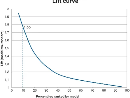
When no model is employed, for any 𝑥% of the sample, the expected proportion of churners is 𝜋̂₀. A good churn classification should be able to give higher probability to churn events compared to non-churn events, hence having more churn events among the events receiving the highest probability. As a result, compared to the case without using any model, lift measures the superiority of a churn classification model to identify more churn events among the events that receive the highest probability from the model (Gur Ali & Ariturk, 2014). A lift chart is illustrated in Figure 5 where the horizontal axis is the percentages of the

(33)

Literature Review on Churn Prediction samples sorted by their probabilities given by the model and the vertical axis is the ratio between the churn ratio in a specific percentile and the churn ratio of the whole population.

Figure 5: Illustration of a lift chart

Lift validates whether the model is able to capture more churners within the top percentiles based on its ranking compared with a random model (Lemmens & Croux, 2006); therefore, a lift of 1 means no lift at all. Figure 5 shows that the lift curve decreases towards 1 when it reaches towards the total population. As a result, 1 is the lower bound of the lift curve.

The popular cut-off used in churn literature when it comes to lift is the top 10%. As the name suggested, top decile lift focuses on the top 10% customers with the highest churn probabilities. Top decile lift is calculated as shown in the formula below:

𝑇𝑜𝑝 𝑑𝑒𝑐𝑖𝑙𝑒 𝑙𝑖𝑓𝑡 = 𝜋̂10% 𝜋̂₀

• 𝜋̂10% is the proportion of churners in the top 10% riskiest customers based on

the model’s prediction

• 𝜋̂₀ is the proportion of churners in the whole population

Take the example in Figure 5, the top decile lift is 1.55, meaning that by selecting the top 10% of customers ranked by the model for a retention campaign, it is possible to target at 55% more potential churners than not using the model. The higher the top decile lift is, the

(34)

better the model is able to capture churners by its ranking; hence top decile lift is claimed to provide managerial suggestions that are straight-forward and actionable (Gur Ali & Ariturk, 2014).

However, researchers who promote profit maximization for the retention campaign criticize churn models that ignore the different costs between Type I and Type II errors because in such cases, the top decile cut-off is merely an arbitrary target size based on the churn probability ranking that ignores the heterogeneity of customers in terms of the generated profitability and the tendency to response to marketing incentives (Lemmens & Gupta, 2013).

(35)

Research Methodology

3 Research Methodology

In order to answer the research question, four methods are employed in this thesis as churn classification algorithms:

• Logistic Regression

• Decision Tree

• Random Forest

• Gradient Boosting

All the four methods will be employed with both multi-period training data and single period training day to create competing models. Specifically, logistic regression and decision tree are used to run the baseline models with single period training data. The other models are then compared with the baseline models in order to answer the research question.

In this section, the four selected algorithms are briefly reviewed. As random forest and gradient boosting belong to the bagging and boosting methods of the ensemble “family”, learning the basics of bagging and boosting helps understand the algorithms developed out of these methods: random forest and gradient boosting.

The main goal of a churn classification model is to train an algorithm on a specific training data set with a vector of independent variables or churn predictors 𝑿= (𝑥1, 𝑥2, … , 𝑥𝑖)

to produce for each observation a binary dependent variable or churn response 𝑌, which takes the values of either 1 for churners and 0 or -1 for non-churners depending on the churn algorithms.

3.1 Logistic Regression

Given the vector 𝑿= (𝑥₁, 𝑥₂, … , 𝑥_𝑖) of independent variables 𝑥_𝑖 as inputs, 𝑔(𝑿) is the linear function of 𝑿.

𝑔(𝑿) = 𝛽0+ 𝛽1𝑥1+ ⋯ + 𝛽𝑖𝑥𝑖

As the goal is to predict the probability of churn, logistic regression returns the binary output 𝑌 that takes the values of either 1 for churners or 0 for non-churners. Let’s denote

𝐹(𝑿) as the probability of churn:

𝐹(𝑿) = 𝑃(𝑌 = 1|𝑿)