A Framework for Assessing the Performance of Pulsar
Search Pipelines
E. van Heerden,
1
?
A. Karastergiou,
2
,
3
,
4
S. J. Roberts
1
1Information Engineering, University of Oxford, Parks Road, Oxford OX1 3PJ, UK2Astrophysics, University of Oxford, Denys Wilkinson Building, Keble Road, Oxford OX1 3RH, UK 3Physics Department, University of the Western Cape, Cape Town 7535, South Africa
4Department of Physics and Electronics, Rhodes University, PO Box 94, Grahamstown 6140, South Africa
Accepted 2016 November 22. Received 2016 November 22; in original form 2016 June 14
ABSTRACT
In this paper, we present a framework for assessing the effect of non-stationary Gaus-sian noise and radio frequency interference (RFI) on the signal to noise ratio, the number of false positives detected per true positive and the sensitivity of standard pulsar search pipelines. The results highlight the necessity to develop algorithms that are able to identify and remove non-stationary variations from the data before RFI ex-cision and searching is performed in order to limit false positive detections. The results also show that the spectrum whitening algorithms currently employed, severely affect the efficiency of pulsar search pipelines by reducing their sensitivity to long period pulsars.
Key words: methods: analytical – methods: data analysis – methods: statistical – (stars:) pulsars: general.
1 INTRODUCTION
Pulsars provide a wealth of information about neutron star physics, the interstellar medium and stellar evolution (Lorimer & Kramer 2005). Furthermore, their clock-like properties allow for sensitive measurements of their orbital dynamics which are used to constrain the equation of state
of ultra-dense matter (Hessels et al. 2006;Demorest et al.
2010), probe the physics of binary evolution and test the pre-dictions of General Relativity (Antoniadis 2014). The con-tinued discovery of new pulsars through pulsar surveys is paramount if we are to improve our understanding of the radio pulsar population as well as expand research in the aforementioned areas. Consequently, pulsar surveys remain a driving force in the field of astrophysics.
Pulsar research has in the past been driven by a number of large-scale surveys carried out with various radio tele-scopes. Surveys of the Galactic plane (Manchester et al. 2001; Johnston et al. 1992), supernova remnants (Seward & Harnden Jr 1982), globular clusters (Manchester et al. 1991) and all-sky surveys (Manchester et al. 1996;Cordes et al. 2006a) have led to the discovery of more than 2200 pulsars.
Pulsar population synthesis models (Lorimer 2011), based on pulsar surveys and the known pulsar population, are used to predict the number of pulsars expected to be
dis-? E-mail: [email protected]
covered in future pulsar surveys (Lorimer et al. 2006;Bates
et al. 2014). These techniques are also used to estimate the number of potentially detectable (i.e. those that are beam-ing towards us as well as bebeam-ing luminous enough) normal pulsars and millisecond pulsars (MSPs) in the Galaxy.
The number of pulsars actually discovered in recent
sur-veys (Swiggum et al. 2014;Lazarus et al. 2015) has fallen
well short of the number predicted by the aforementioned estimation techniques. It was predicted that the Arecibo PALFA Precursor survey (Swiggum et al. 2014) should have detected490+−160115 normal pulsars and12+−705 millisecond pul-sars (MSPs) by the beginning of 2014, but managed to detect
only283normal pulsars and 31 MSPs. The full PALFA
sur-vey, when complete, is expected to have detected1000+−330230
normal pulsars and30+−20020 MSPs. However, close to
comple-tion it has only managed to detect∼443normal pulsar and
∼40MSPs respectively (Lazarus et al. 2015). It is worth
not-ing that the largest discrepancy between predictions and de-tections is for normal pulsars, i.e. pulsars with long periods. Furthermore, it is estimated that there are between 82,000 to 143,000 detectable normal pulsars and 9,000 to 100,000 detectable MSPs in the Galactic disk alone (Lorimer et al. 2006;Swiggum et al. 2014), yet to date we have only discov-ered some 2200 pulsars (Hobbs et al. 2004). The deficiencies in pulsar detections have been attributed to RFI and scintil-lation (Lorimer 2011), both these effects are not addressed in current population synthesis models (Levin et al. 2013).
Electromagnetic radiation with frequencies between
circa 10 kHz and 100 GHz is referred to as radio frequency (RF). Radio frequency interference (RFI) in the context of a pulsar survey is any signal or disturbance emitted from a man-made source either extra-terrestrial or terrestrial that corrupts the measurements of data obtained. The spatial and temporal variability of RFI make it difficult to iden-tify and to mitigate. If RFI is not dealt with then spurious trends may occur in the data collected, thereby decreasing the signal to noise ratio (SNR) and making it more difficult, or impossible, to detect new pulsars.
All-sky pulsar surveys, such as the Arecibo PALFA sur-vey, are more often than not conducted in the L-band (the 1 to 2 GHz range of the radio spectrum), more specifically the frequency range 1.2 GHz to 1.6 GHz (Lazarus et al. 2015;Burgay et al. 2006). The frequency range 1.2 GHz to 1.6 GHz happens to overlap with frequencies that have been earmarked for other applications such as satellite navigation, telecommunication, aircraft surveillance, amateur radio and digital audio broadcasting (Regulations 2008). Most of the aforementioned RFI sources severely decrease the sensitivity of surveys conducted in the L-band.
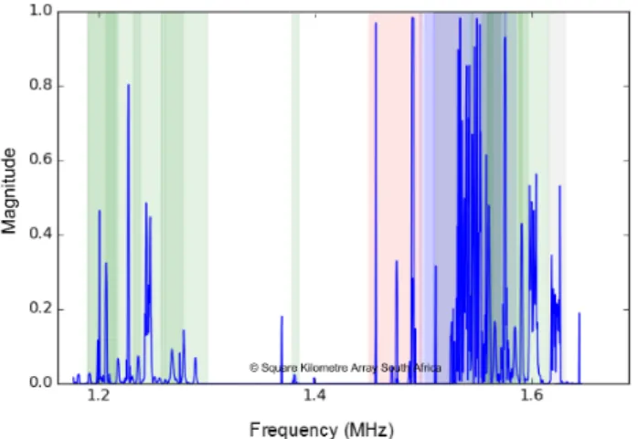
Spectrum occupancy in the L-band, depicted in Fig-ure 1, is dominated by RFI mainly from satellites. The
colours in Figure 1 represent interference from different
satellites: red - Afristar, yellow - Thuraya, blue - Inmarsat,
cyan - Satellite Radio, grey - IRIDIUM, green - {Galileo,
Beidou, GPS, GLONASS}and grey -{Fengun, Meteosat}.
Figure 1.Typical spectrum occupancy in the L-band.Source: Square Kilometre Array South Africa
In a recent study by Lazarus et al. (2015), synthetic
pulsars with various periods and pulse widths were injected into actual PALFA survey data with the aim to assess the
effect of RFI and red noise1 on the survey sensitivity. The
study found that there is a significant degradation in
sensi-tivity of between10 %and a factor of 2 for pulsars with spin
periods between 0.1 s and 2 s and dispersion measure (DM)
> 150 pc cm−3 due to red noise induced by RFI, receiver
gain fluctuations and opacity variations of the atmosphere. Additionally, a population synthesis analysis based on the
1 Red noise is a type of signal noise with a power spectral density inversely proportional to f2, which means it has more energy at lower frequencies.
empirical survey sensitivity found that35±3 %of pulsars,
with predominantly long periods, are missed compared to expectations which are based on the theoretical sensitivity curves as derived from the radiometer equation. With these results the authors conclude that the reduced sensitivity to long-period pulsars is mainly attributed to red noise. All the results were obtained despite applying a red noise suppres-sion algorithm.
In this paper we show, supplementary to theLazarus
et al.(2015) study, that frequency dependent noise such as red noise indeed reduces the SNR of long-period pulsars and increases the number of false detections (Lyon et al. 2016). Moreover, we offer an explanation as to how the red noise
suppression technique in theLazarus et al.(2015) paper
ac-tually contributed to the reduced sensitivity of long-period pulsars by explaining what the algorithm does and quanti-fying the loss of signal to noise ratio when the algorithm is applied.
It is evident, from the number of pulsars missed, that RFI and frequency dependent noise greatly affect the sensi-tivity of radio telescopes to normal pulsars, i.e. pulsars with long periods. Therefore, the aims of this study are:
(a) to quantify the effect that non-stationary Gaussian noise and RFI has on the performance of pulsar search pipelines;
(b) to examine the effectiveness of the current spectrum whitening methods available in pulsar search software suites;
(c) to determine if detrending the data with a moving av-erage filter before searching for pulsars is effective; (d) to examine the effectiveness of the current RFI
detec-tion and mitigadetec-tion methods available in pulsar search software suites.
(e) to investigate the reduction in sensitivity as a func-tion of both the correlafunc-tion length of the non-stafunc-tionary noise and the pulse period.
We start in§ 2.2by describing the building blocks of
a typical pulsar search pipeline for normal pulsars. There exist various software implementations of this pipeline. The
ones used in this analysis are introduced in§2.3. Although
these software packages differ in a number of ways, the way in which they deal with frequency dependent noise is of
par-ticular interest for this study. Therefore, in section § 2.4
the different spectrum whitening algorithms available in the software packages considered are mathematically described. The method used for generating the synthetic filterbank files
with non-stationary Gaussian noise are detailed in § 3.1.1
and the RFI added to some of the files can be found in
§3.1.2. In§3.2.1 to§ 3.2.4we introduce the experimental framework we used for generating and processing filterbank files containing different noise processes.
The aim of this framework is to assess the ability of different pulsar search pipelines to detect pulsars embedded in non-stationary Gaussian noise amidst RFI. It is worth
noting that this study differs from theLazarus et al.(2015)
study in that the aim is to quantify the sensitivity of dif-ferent pulsar search pipelines as a function of noise correla-tion length and pulsar spin period, whereas the latter aimed at quantifying the Arecibo PALFA survey’s sensitivity as a function of DM and pulsar spin period. Finally, the results,
2 SEARCH PROCESS FOR NORMAL PULSARS
In order to determine how phenomena like RFI and non-stationary noise can hinder pulsar detections it is necessary to first understand the nature of the acquired data and the functionality of each of the building blocks that form part of a pulsar search pipeline. Therefore, a detailed descrip-tion of a typical pulsar search pipeline is presented in this section. Two existing software implementations of the pul-sar search pipeline and a detailed algorithmic description of the spectrum whitening techniques available in each of them are also presented here. Different configurations of these soft-ware suites are used in a subsequent section to process pulsar data where the results will be used to assess their abilities to deal with non-stationary noise and RFI.
2.1 Search data
The data that are searched for pulsars are time series of total power per frequency channel typically referred to as filter-bank data. The number of frequency channels, the temporal resolution and the dynamic range (i.e. 1-bit, 8-bit or 16-bit) of the data are unique to each survey.
Files that contain filterbank data are currently pro-cessed off-line; however, with the increase in scope and sen-sitivity of future surveys it will become infeasible to store the raw data for off-line processing due to capacity and in-put/output constraints. Hence, the need for a paradigm shift from off-line to real-time processing of survey data.
Real-time processing entails block-wise dedispersion for the purposes of rapid reporting of Fast Radio Burst (FRB) detections, which constitute a byproduct of pulsar searches. The time duration of each block depends on the dispersion measure search and the observing frequency, and is likely to be of order a few seconds for typical searches. RFI cleaning must happen prior to dedispersion. Thereafter, all frequency information is lost and likewise the opportunity to detect and mitigate RFI in the time-frequency plane. The relevant timescale on which any RFI excision technique needs to op-erate is therefore more likely to be related to the FRB de-tection buffer size, rather than the full integration required for periodicity searches.
2.2 Pipeline for a standard pulsar search
Detecting radio pulses produced by pulsars is an intrinsi-cally difficult task due to their narrow duty cycles, low sig-nal strengths, dispersion effects and the presence of non-Gaussian noise.
Numerous techniques have been developed to overcome some of the difficulties highlighted above. These techniques are combined to form the standard pulsar search pipeline.
The typical pipeline used for the processing of filterbank
files consists of nine stages as depicted in Figure 2. The
pipeline starts with noisy filterbank files (Figure 2.1) that
may or may not contain a pulsar.
Each filterbank file is examined for narrowband RFI signals, which are excised by replacing the affected samples with constant values chosen to match the median bandpass
(Figure2.2) (Lazarus et al. 2015).
The corrected filterbank files are then dedispersed for a
number of trial dispersion measure (DM) values to compen-sate for the dispersion induced by the interstellar medium
(Figure2.3) (Lorimer & Kramer 2005). The zero-DM time
series is used to identify and mitigate broad band RFI (Fig-ure2.4) that went undetected by the narrow band RFI exci-sion process. After mitigating broad band RFI, the Fourier transform of each dedispersed time series is computed (Fig-ure2.5).
The power spectrum is whitened (Figure 2.6) so that
the response is as uniform as possible, i.e., mitigating fre-quency dependent noise, subtracting a running median and normalising the local root mean square (rms) of the power spectrum such that it has a zero mean and unit rms. A whitened power spectrum is preferred, because estimating the significance level of any signal present is relatively easy. Different techniques have been implemented to whiten the spectrum and these will be described in more detail in
sec-tion2.4.
The next stage of the pipeline concerns identification of periodic RFI. Known periodic signals which are present all or most of the time, such as power lines carrying alter-nating current and communication systems such as airport radar systems are flagged with their harmonics and their bandwidths determined. These interferences are mitigated
by creating a spectral mask (see Figure2.7). This mask
con-sists of a list of all the Fourier bins affected and which should be ignored in all subsequent processing.
Radio pulses from pulsars generally have narrow duty cycles which, in the Fourier domain, results in the power to be distributed between the fundamental frequency and a number of harmonics (van Heerden et al. 2014). Therefore, to take full advantage of the power contained in the har-monics the whitened spectrum is harmonically summed by adding the higher harmonics to the fundamentals. The orig-inal power spectra as well as the composite spectra formed by summing 2, 4, 8 and 16 harmonics (Lyne & Graham-Smith 2012) are each searched for periodicities (Figure2.8) (Cordes et al. 2006a). The best candidates from each trial DM are saved.
After all the time series have been processed, a list of pulsar candidates is compiled. This list is pruned by
post-processing procedures (Figure2.9) ranging from sifting and
folding to sophisticated machine learning candidate selection (Lazarus et al. 2015). The most promising pulsar candidates are saved for future observation and follow-up (Cordes et al. 2006a).
2.3 Pulsar search software
The pulsar search pipeline described above is available in
a number of pulsar search software packages: SIGPROC
de-veloped by Lorimer (Lorimer 2001), PRESTO developed by
Ransom (Ransom 2011),PEASOUP developed by Barr (Barr
2013) andPULSARHUNTERdeveloped by Keith (Keith 2007).
The two most frequently used packages are SIGPROC and
PRESTO, both of which are freely available and well tested. Together they have been responsible for the discovery of most of the pulsars known today. We refer the interested
reader toCordes et al.(2006b),Rane et al.(2016), Stovall
et al.(2014) andLazarus et al.(2015) for a comprehensive discussion of how these two pipelines are typically used in real pulsar surveys.
Figure 2.Schematic illustration of a typical pulsar search pipeline, see text for details.
There are three main differences betweenSIGPROC and
PRESTO. Firstly, the manner in which they search for pulsars that orbit a companion, namely binary pulsars. Radio pulses from binary pulsars typically exhibit Doppler shifts in their rotational period, caused by the acceleration of the pulsar around its companion. To be efficient, these shifts need to be
accounted for in the so-called acceleration searches.PRESTO
performs acceleration searches in the Fourier domain (Ran-som 2001).SIGPROCon the other hand does time-domain
re-sampling to carry out acceleration searches. Secondly,
SIG-PROClooks for harmonically related signals in the amplitude
spectrum, whereasPRESTOuses the power spectrum to
iden-tify possible pulsar candidates (Lorimer & Kramer 2005).
Lastly,SIGPROCuses SNR as a metric to identify peaks in the
normalised power spectrum whereasPRESTOuses the
Gaus-sian significance (adjusted for the number of trials searched) of the peaks as a metric under a white noise assumption. Hereinafter, the terms SNR and Gaussian significance shall
be collectively referred to asdetection significance.
2.4 Spectrum whitening
A stochastic process is considered white if and only if it is stationary and independent at all points. As a consequence, the power spectral density of a white process is uniformly distributed across the whole available frequency range. A non-white process is instead characterised by a given distri-bution of the power per unit frequency along the available frequency bandwidth (Lazarus et al. 2015). A whitening op-eration on any non-white process entails forcing said process to adhere to the conditions described above for a white pro-cess.
In the case of pulsar searching, well-behaved white noise is sought after, because it simplifies any attempt at estimat-ing the significance levels of any signal present in the data and consequently makes detection easier. Hence, it is stan-dard practice to whiten the power spectral density by sup-pressing frequency-dependant noise, in particular red noise, so that the response to noise is as uniform as possible.
The spectrum whitening techniques implemented in
SIGPROC and PRESTO are similar in that they aim to nor-malise the spectrum. However, the way in which these tech-niques algorithmically operate in normalising the spectrum is quite different. The different whitening options available inSIGPROCandPRESTOare mathematically described in the two subsequent sections.
2.4.1 Spectrum whitening in SIGPROC
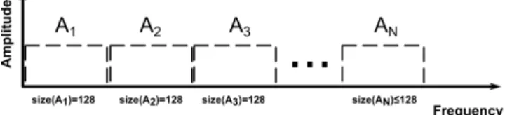
In SIGPROC there are three spectrum whitening
options for the SEEK function. In all three
ap-proaches the spectrum is divided into blocks of
max{128,(number of spectral data points/400000)} Fourier
bins. The simulation parameters of this analysis resulted in the number of Fourier bins per block to be consistently 128 and thus for all subsequent explanations we assume that the spectrum is divided into blocks of 128 Fourier bins as
depicted in Figure3.
Figure 3.Amplitude spectrum partitioning for the whitening algorithm implemented inSIGPROC, see text for details.
The algorithms implemented for the three options in
SIGPROCare:
• Option 1:
The default whitening algorithm executed when the
func-tionSEEKis called computes the mean and corrected sample
standard deviation,s=q1
(N−1)∑Ni=1(xi−x¯)2, for each of
the blocks A1,...,AN in Figure 3. The mean is subtracted
from each Fourier bin in the block, whereafter the bins are scaled by the corrected sample standard deviation of that particular block. The algorithmic steps are detailed in
Algo-rithm1.
Algorithm 1SIGPROC:default
1: fori=1, ...,Ndo
2: µi=mean(Ai)
3: si=corrected standard deviation(Ai)
4: Anewi = (Aoldi −µi)/si 5: end for
• Option 2:
The whitening algorithm executed when the functionSEEK
is called with the flag -submn is identical to Algorithm 1
except for one difference. The blocks A1,...,AN in Figure3
are scaled with the root mean square (rms) of that particular block instead of the corrected sample standard deviation.
• Option 3:
The whitening algorithm executed when the functionSEEK
is called with the flag -submjk computes the mean and
corrected sample standard deviation for each of the blocks
A1,...,ANin Figure3. Thereafter, the gradients of the mean
and corrected sample standard deviation between adjacent blocks of 128 Fourier bins are computed. For each Fourier bin j=1, ...,128in a block the mean is subtracted and the result scaled with the corrected sample standard deviation, where-after the mean and corrected sample standard deviation is updated with the calculated gradients for that particular
Algorithm 2SIGPROC:submjk
1: fori=1, ...,N do
2: µi=mean(Ai)
3: µi+1= mean(Ai+1)
4: si=corrected standard deviation(Ai)
5: si+1=corrected standard deviation(Ai+1) 6: slopemeani= (µi+1−µi)/128
7: slopesi= (si+1−si)/128 8: for j=1, ...,128in Ai do 9: Anewi [j] = (Aiold[j]−µi)/si
10: Update:µi=µi+slopemeani
11: Update: si=si+slopesi
12: end for 13: end for
2.4.2 Spectrum whitening in PRESTO
InPRESTO there is only one spectrum whitening technique implemented to suppress frequency dependent noise (Ran-som et al. 2002). The median power level is measured in blocks across Fourier bins and then multiplied by log 2 to convert the median value to an equivalent mean level assum-ing that the powers are distributed exponentially. There-after, the measured mean power values (variable P in
Algo-rithm3) are used to compute the slope between two adjacent
Fourier bins which in turn is used to normalise the complex
Fourier amplitudes (variable A in Algorithm3).
The number of Fourier frequency bins per block starts
with 6 and increases logarithmically to 200, see Figure 4.
Thus, for frequencies where there is little coloured noise the number of bins used per block are 200. The algorithmic steps for the spectrum whitening technique implemented in
PRESTOare detailed in Algorithm3.
Figure 4.Power spectrum partitioning for the whitening algo-rithm implemented inPRESTO, see text for details.
Algorithm 3PRESTO:default
1: fori=1, ...,N do
2: µi=median(Pi)/log 2
3: µi+1= median(Pi+1)/log 2
4: slopei= (µi+1−µi)/(size(Pi) +size(Pi+1)) 5: lineoffset=12(size(Pi) +size(Pi+1)) 6: for j=1, ...,size(Pi)do
7: Update: lineval=µi+slopei×(lineoffset−j)
8: Update: scaleval=1/√lineval
9: Update:Re(A)newi [j] =Re(A)oldi [j]×scaleval
10: Update:Im(A)newi [j] =Im(A)oldi [j]×scaleval
11: end for 12: end for
Irrespective of the red noise suppression algorithm being
applied,PRESTO by default normalises the power spectrum
using median blocks before performing harmonic summing and searching.
3 METHODOLOGY
Pulsar software currently available for generating synthetic pulsar data as well as the detection and timing thereof, as-sumes that the noise present in the signals acquired by radio telescopes is additive white Gaussian noise. This assump-tion ignores the fluctuating nature of the sky temperature
(Lorimer & Kramer 2005;Nice et al. 1995) as well as the
ef-fects that RFI have on the noise baselines of the data. Con-sequently, it is poorly understood how the aforementioned phenomena, which are clearly non-stationary, affect the abil-ity of pulsar search pipelines to detect pulsars. Hence, the
need for software to emulate these phenomena (see § 3.1)
and a framework whereby their effect on the ability of pul-sar search pipelines to detect pulpul-sars can be investigated and
quantified (see§3.2).
3.1 Synthetic file generation
In section§3.1.1we present the low-pass filter that was
in-spired by a Gaussian Process (Rasmussen & Williams 2006) to generate synthetic filterbank files with non-stationary
noise baselines. Additionally, in section§3.1.2 we describe
the choice of RFI that we injected into a subset of the syn-thetic filterbank files.
3.1.1 Non-stationary Gaussian noise
Filterbank files contain quantised power values computed by superimposing tens or even hundreds of single Nyquist power
measurements (see Equation1). The power measurement of
a single Nyquist sample is computed from the real and imag-inary parts of the raw voltages associated with either linear or circular polarised electromagnetic waves acquired by ra-dio telescopes. The power measurement of a single Nyquist sample is given as:
Power=Xreal2 +Ximag2 +Yreal2 +Yimag2 , (1)
where X and Y are either the horizontal and vertical
com-ponents of linear polarisation or the left and right handed components of circular polarisation.
The power values found in filterbank files comprise both signal and noise. The noise levels in the filterbank files are proportional to the overall system temperature which is af-fected by RFI, the sky temperature and the receiver temper-ature. During an observation various objects and RFI with different brightness levels are encountered so the duration and magnitude of the non-stationarity associated with each of these phenomena differ greatly.
In order to generate a time series with correlated sam-ples, i.e. a varying noise baseline, we constructed a low-pass
filter (see Equation2) and convolved it with random samples
drawn from a Gaussian distribution with zero mean and unit variance (N (0,1)) (see Equation3), whereε=1×10⁻⁵,tis
the sampling interval andN the number of samples in the
w with samples correlated over length scales defined by λ
and magnitudes proportional toh(see Equation4).
u:=h2exp −t λ 2 ∀t∈R such that u>ε (2) v:=z1,z2, ...,zN∼N (0,1) (3) w=u∗v (4)
In order to generateNdata points which are correlated
over long length scales (i.e.λ>>) requiresNrandom
sam-ples drawn from a standard normal distribution (N (0,1))
to be convolved with a finely sampled low-pass filter which is compact on a large interval. Consequently, convolving two large vectors is computationally very expensive. To circum-vent this challenge we generate data points with the required correlation length by convolving a fraction of the random samples drawn from a standard normal distribution with a coarsely sampled low-pass filter and then interpolating be-tween the resultant points to produce a time-series with the desired number of points.
The vectorwgenerated by convolving the low-pass filter
with samples drawn from a standard normal distribution is not always positive. However, for the purpose of these exper-iments non-negative samples are desired because the stan-dard deviation of the baseline drift needs to be proportional
to the square root of the mean. Therefore, a new vectorgis
defined:
g=w−min(w), (5)
such that the offset is equal to zero and all the values are non-negative.
The mean vectorgis used to generate samples for the
vectorsXreal,Ximag,Yreal,Yimag: Xreal,Ximag,Yreal,Yimag
i.i.d.
∼ N (g,√g), (6)
such that the power for each sample in the synthetic
filter-bank file can be computed using Equation1.
A large value for the length-scale variableλ of the
low-pass filter results in a slow drifting baseline as depicted in
Figure5a. As the value ofλ deceases the baseline drifts
be-comes more capricious as depicted in Figure5bto Figure5e.
3.1.2 RFI injected
For the experiments aimed at investigating the effects of RFI on the performance of pulsar search pipelines we injected
the same RFI into all the filterbank files, see Figure6. The
choice of injected RFI was obtained by studying spectrum occupancy data from the KAT-7 radio telescope over several
months (see Figure1) and cross-correlating that with the
L-band spectrum allocation as determined by the International Telecommunication Union (ITU) (Regulations 2008). The RFI injected include:
(a) broadband periodic RFI with a period of 0.02 s and a duty cycle of 50 %,
(b) narrowband periodic RFI with a period of 12 s and a duty cycle of 25 % affecting the frequency channels 1.266 GHz to 1.276 GHz,
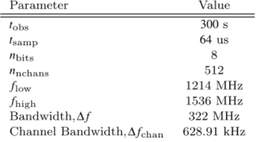
Table 1.Simulated observation parameters
Parameter Value tobs 300s tsamp 64us nbits 8 nnchans 512 flow 1214 MHz fhigh 1536 MHz Bandwidth,∆f 322 MHz
Channel Bandwidth,∆fchan 628.91 kHz
(c) several instances of narrowband RFI with random du-rations affecting the frequency channels identified from
the RFI characterisation plot in Figure1.
Various routines exist in current pulsar search pipelines for excising bright RFI, but the effect of weak and unknown sources of RFI are unbeknownst to us. Therefore, the mag-nitudes of the various instances of injected RFI were delib-erately chosen to be within one sigma of the baseline such that the effect of weak RFI on pulsar search pipelines could be investigated. The percentage of samples affected by RFI
is12 %for each filterbank file.
3.2 Framework for Pulsar Search Pipeline Analysis
In this section a framework to generate and process non-stationary noise files with RFI is introduced. This frame-work allows for the understanding of how non-stationary noise processes with different correlation lengths can impede the detection of pulsars with specific periods. Additionally, it contributes to the understanding of how RFI can pass undetected through current pulsar search pipelines and the consequences of not mitigating these spurious sources of in-terference.
The generation part of this framework include the
syn-thetic observation parameters (see§3.2.1), the experimental
design specifics for each experiment (see§3.2.2) and the
pe-riods of the pulsars injected for this analysis (see§3.2.3).
The processing part of this framework includes the
dif-ferent configurations ofSIGPROCandPRESTOthat were
anal-ysed (see§3.2.4).
3.2.1 Simulated observation parameters
The observation parameters that were used for generat-ing the synthetic filterbank files were chosen to match the Arecibo PALFA survey (Lazarus et al. 2015) parameters and
are summarised in Table1.
3.2.2 Experiments
The experiments that we designed for analysing various
con-figurations of SIGPROC and PRESTO are summarised in
Ta-ble2.
The design of experiments 1 to 4 is such that each one emulates a blind pulsar survey. Each experiment comprises one hundred simulated pointings with a subset of these con-taining a pulsar. The differences between the experiments
(a)λ=100s (b)λ=10s
(c)λ=1s (d)λ=0.1s
(e)λ=0.01s
Figure 5.Examples of dedispersed time series that correspond to the five correlation lengths used to simulate non-stationary noise processes. Black represents the actual signal in the filterbank file, orange the mean and pink the standard deviation (1σ) of the dedispersed
time series. The correlation length decreases from (a) 100 s to (e) 0.01 s.
Table 2.Summary of the experiments conducted
Experiment # Files # Pulsars Noise h λ (s)
1. Stationary 100 15 Stationary Gaussian -
-2. Non-stationary 100 15 Non-stationary Gaussian 0.1, 0.2, 0.3, 0.4 0.01, 0.1, 1.0, 10.0, 100.0
3. Stationary +RFI 100 15 Stationary Gaussian -
-4. Non-stationary +RFI 100 15 Non-stationary Gaussian 0.1, 0.2, 0.3, 0.4 0.01, 0.1, 1.0, 10.0, 100.0 5. All pulse periods perλ 75 75 Non-stationary Gaussian 0.1, 0.2, 0.3, 0.4 0.01, 0.1, 1.0, 10.0, 100.0 6. All pulse periods perλ+ RFI 75 75 Non-stationary Gaussian 0.1, 0.2, 0.3, 0.4 0.01, 0.1, 1.0, 10.0, 100.0
Figure 6.The RFI injected into each filterbank file.
are the type of noise processes simulated and whether RFI is present of not.
Experiment 1 comprises one hundred files with station-ary Gaussian noise. Fifteen of the hundred files contain an
injected pulsar (see Table3) and the remainder are without.
The results from experiments 2 to 4 will be benchmarked against the results of experiment 1 because of its idealised noise process and lack of RFI.
Experiment 2 comprises one hundred files with non-stationary Gaussian noise. Fifteen of the aforementioned
files contain an injected pulsar that is unique (see Table 3)
and the remainder of the files are without a pulsar. The non-stationary Gaussian noise processes were generated
ac-cording to the procedure described in §3.1.1. Note, every
noise process is unique in that each one is defined by a
different non-stationary vector, g, and the additive
Gaus-sian noise has zero mean and variance proportional to the
square root of the non-stationary vector (see Equation 6).
The length scales,λ, for the non-stationary variability of the
noise baselines range from10−2s to102s in factors of 10, i.e.
twenty files were generated perλ. Consequently, each file
ex-hibits a unique variation because of the stochastic nature of the generation process despite having the same correlation length.
The correlation lengths can be chosen to represent any timescale that we could consider to have an effect on the survey sensitivity to periodic pulsars, and could result from instrumental variability, to environmental effects and RFI. The power spectrum of a non-stationary noise baseline with a given correlation length will contain more power in the frequencies that correspond to that length. For this rea-son, we choose our length scales to sample a broad range that is relevant to the pulse periods searched, as mentioned above. Comparing the results from experiment 2 with the results of experiment 1 enables the quantification of the ef-fect that non-stationary Gaussian noise has on the perfor-mance of pulsar search pipelines. Moreover, experiment 2 allows for the determination of the effectiveness of the
spec-trum whitening techniques described in§2.4and whether or
not detrending the data with a moving average filter before searching for pulsars is effective.
Experiment 3 is identical to experiment 1 except for
the addition of RFI (see§ 3.1.2). The experimental design
of experiment 3 serves to investigate the ramifications when
weak RFI (see § 4.4) passes undetected through a pulsar
search pipeline. Furthermore, it serves to investigate the ef-ficacy of RFI detection and mitigation algorithms currently employed.
Experiment 4 is identical to experiment 2 except for the
Table 3.Synthetic pulsar properties
Parameter Value
Period(ms) 1.102 2.218 5.218 10.870 18.505 61.965 126.175 286.555 533.320 850.158 1657.496 2643.410 3927.013 5580.899 9964.532
Amplitude All pulsars are detectable with a detection significance of∼12inSIGPROCin the presence of stationary Gaussian noise when processed with pipeline H inSIGPROC. Duty cycle 12%(fixed)
Dispersion measure 68
addition of RFI (see § 3.1.2). Comparing the results from
experiment 4 to the results of experiments 1, 2 and 3 re-spectively serves to quantify the combined effect that non-stationary Gaussian noise and RFI have on the performance of pulsar search pipelines and to deduce which phenomenon has the greatest impact on said performance.
Experiment 5 comprises seventy five files in total, fifteen
files per correlation lengthλ (see Table2). Each one of the
pulsars in Table 3 was separately injected into the fifteen
files with the same correlation length and this was repeated for all five values ofλ.
Experiment 6 is identical to experiment 5 except for
the addition of RFI (see§3.1.2). The experimental design
of experiments 5 and 6 serves to investigate the reduction in sensitivity of pulsar search pipelines as a function of both the correlation length of the non-stationary noise and the pulse period of a pulsar.
Lastly, experiments 2, 4, 5 and 6 are repeated for four
different values of the magnitude parameter h defined in
Equation2, namelyh=0.1,0.2,0.3,0.4.
3.2.3 Pulsar properties
The properties of the fifteen pulsars that were randomly injected into the synthetic filterbank files were taken in part from the Arecibo sensitivity study (Lazarus et al. 2015) and
are summarised in Table3.
A pulse with the profile of pulsar PSR B0833-45 at 1.4 GHz obtained from the EPN-database (Lorimer et al. 1998)
with a duty cycle of12 %was injected into all the files.
3.2.4 Pulsar search pipeline configurations
All of the files generated for the experiments described in
Table 2 were processed by both SIGPROC and PRESTO, i.e.
twelve different configurations ofSIGPROC(see Table4) and
eight different configurations of PRESTO (see Table5) were
used to search every single synthetic file. Because the aim with this analysis is not to investigate sensitivity as a func-tion of DM, all the files were dedispersed at the correct DM.
SIGPROC by default removes the baseline of a dedis-persed time series by linearly detrending the time series
un-less the flag-nobaselineis set when thededisperse
func-tion is called. In addifunc-tion to the opfunc-tion available inSIGPROC
for detrending the baseline, a 10 s moving average filter was implemented as a second option for normalising the base-line of a dedispersed time series. The red-noise mitigation
Table 4.The twelveSIGPROCpipeline configurations used to pro-cess all the files in this analysis.
Pipeline Baseline Red-noise mitigation
A Removed default B Removed submn C Removed submjk D Removed -E Intact default F Intact submn G Intact submjk H Intact
-I Moving average filter default
J Moving average filter submn
K Moving average filter submjk
L Moving average filter
-techniques applied in the differentSIGPROCpipelines are
de-scribed in§2.4.
To process all the files withSIGPROCthe following
func-tions and their associated flags were called:
(a) function dedisperse with the flags -d, -o and
with/without-nobaseline,
(b) functionseek(number of summed harmonics is 16) with
the flags-zand-submn/-submn/-submn,
(c) functionbestwith flag-s8.
The functionbestinSIGPROCproduce a ’.lis’ file which was
searched for possible candidates based on the SNR of the peaks.
The RFI mask configuration option in Table5refers to
the RFI mask computed inPRESTOwhen therfifind
func-tion is called. In this analysis an RFI mask was computed and applied to each synthetic filterbank file at integration intervals of 8 s. An integration time of 8 s was chosen to resemble typical real-time processing intervals. The default values for the time and frequency rejection thresholds in therfifind function was selected. A moving average filter of 10 s was also implemented as a processing step in the
PRESTOpipelines. Lastly, details of the red-noise mitigation
technique inPRESTOcan be found in§2.4.
To process all the files withPRESTOthe following
func-tions and their associated flags were called:
(a) function prepdata with the flags -dm, -o and
with/without the flag-mask
(b) functionrealfft,
(c) functionzapbirdswith the flags-zapand-zapfile,
(d) functionaccelsearchwith the flags-sigma 1.0,
-flo 0.1,-zmax 0 (acceleration searching was turned
off by setting the flag -zmax 0) and-numharm 16(i.e.
the number of summed harmonics is 16).
The accelsearch function in PRESTO produce an ACCEL file which was searched for possible candidates based on the Gaussian significance of the peaks under the assumption of pure white noise.
4 RESULTS
The results are organised according to the aims set forth in
the introduction (see§1) of this paper.
Table 5.The eightPRESTOpipeline configurations used to process all the files in this analysis.
Pipeline RFI Moving average Red-noise
mask filter mitigation
A X X X B X X X C X X X D X X X E X X X F X X X G X X X H X X X
The heuristics used for quantifying the results are: (a) a signal is considered a candidate if its detection
signif-icance is greater than the default detection threshold in
SIGPROCorPRESTO,
(b) injected pulsars are considered discovered when (a) holds true AND if the difference between the periods of the discovered and injected signals are less than the allowederror, i.e.:
|Perioddiscovered−Periodinjected| ≤error, where error=0.02ms if period≤10ms
error=0.20ms if10ms<period≤100ms error=2.00ms if100ms<period≤1000ms error=20.0ms if1000ms<period≤10000ms (c) the discoveries from (b) are validated by visual
inspec-tion of their folded profiles produced by folding the in-verse Fourier transform of their whitened spectra at the detected periods. At this stage a detection is rejected if the folded profile does not resemble a real pulsar, (d) determining whether a pulsar was detected or not the
non-fundamental harmonics were not considered, (e) harmonically related candidates are removed and,
(f) only candidates with 1ms≤period≤10 s are
consid-ered.
For the directSIGPROCandPRESTOcomparisons the
ex-act same files were searched by both routines.
The sensitivity of a pipeline refers to the ability of the pipeline to detect the fifteen randomly injected pulsars ex-pressed as a percentage. The number of false positives de-tected per true positive is the total number of false positive candidates detected across all hundred files divided by the number of true positives detected.
Note that all the results presented here should be inter-preted as per DM.
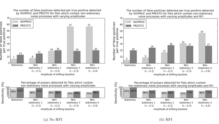
4.1 Non-stationary Gaussian noise and RFI The results of processing the synthetic files from the
emu-lated blind surveys (see experiments 1-4 in Table 2) with
the default pulsar search pipelines of SIGPROC and PRESTO
are shown in Figure7. Note, the metric used in this section
to express the performance of each pipeline is the number of false positives detected for every true positive detected across all 100 files for each experiment.
The number of false positives per true positive detected bySIGPROC increases approximately proportionally with a
linear increase in the amplitude of the non-stationary noise
(see Figure7a). This trend is also visible in Figure7bwhen
RFI is injected. Hence, the defaultSIGPROCpipeline is very
sensitive to non-stationary noise.
The number of false positives detected per true positive by PRESTO is unaffected by the type and amplitude of the noise process present in the files, i.e. the number of false positives detected per true positive is almost constant irre-spective of the amplitude of the non-stationary noise (see
Figure7a). However, the number of false positives detected
per true positive byPRESTOis slightly higher when weak RFI
is present (see§4.4) compared to when no RFI is injected.
The sensitivity of SIGPROCand PRESTO can be seen in
Figure 7a to decrease by at least 20 % and 7 %
respec-tively in the presence of non-stationary noise compared to
the stationary noise case. The20 %and7 %losses recorded
in sensitivity were averaged over all the pulse periods; how-ever, the long period pulsars were much more affected. Note, the amplitudes of the injected pulsars were chosen such that
they are detectable at a SNR of ∼12 in the presence of
white noise when processed with pipeline H inSIGPROC(see
Table3); however, the addition of any (significant) amount
of non-stationary noise rendered the pulsars undetectable. Consequently, there is no correlation visible between sensi-tivity loss and the non-stationary noise amplitude.
There is no correlation between the loss in sensitivity of
SIGPROCand the amplitude of the non-stationary noise when weak RFI is present. Interestingly, the presence of weak RFI
leads to an increase in the sensitivity of SIGPROC for the
stationary noise case with RFI compared to the stationary noise files without RFI. Similarly, there is an increase in sensitivity for the non-stationary 4 case when RFI is present compared to the no RFI case.
Comparing the sensitivity ofPRESTOin Figure7ato the
sensitivity in Figure7bit becomes apparent that PRESTOis
not sensitive to weak RFI. The highest sensitivity
attain-able with PRESTO for files containing weak RFI and
non-stationary noise is 73 %; furthermore, a direct comparison
reveals thatPRESTO’s sensitivity is on average 11 %better
thanSIGPROC’s sensitivity.
4.2 Spectrum whitening methods
The power versus log-frequency plot in Figure8shows the
power spectrum density of two non-stationary Gaussian
noise processes with correlation lengths λ=1 s (red) and
λ =100 s (blue) as well as for a stationary Gaussian noise
process (black). It is evident from Figure8that the power
spectrum density of a non-stationary process diverges from the desired flat power spectrum density of a stationary white noise process as the correlation length of the non-stationary process shortens.
With Figure8in mind, four spectrum whitening
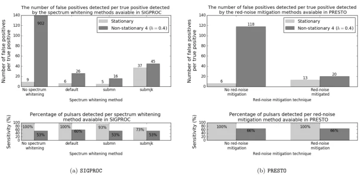
meth-ods (see§2.4) were assessed and the results can be seen in
Figure9. The spectrum whitening techniques in both
SIG-PROC and PRESTO reduce the number of false positives de-tected per true positive significantly compared to the case when no spectrum whitening is applied. In the presence of
non-stationary noise the sensitivity of SIGPROC improved
slightly from 53 % to 60 % when the default spectrum
whitening method was applied but the other methods had
no effect on sensitivity (see Figure 9a). The sensitivity of
PRESTOis unchanged when the spectrum whitening method is applied compared to no spectrum whitening.
4.3 De-trending the data before processing
De-trending the baseline inSIGPROCwith either a 10 s
mov-ing average filter or the built-in de-trendmov-ing method led to an increase in the number of false positives detected per true positive compared to when the baseline was left intact
(see Figure10a). However, the 10 s moving average filter did
improve the sensitivity by6 %.
De-trending the baseline inPRESTOwith a 10 s moving
average filter reduced the number of false positives detected
per true positive and increased PRESTO’s sensitivity with
7 %(see Figure10b).
These results hint at the improved sensitivity attainable when the file contains both a baseline with long correlations and a slowly pulsating pulsar, i.e. removing the baseline sig-nificantly improves the sensitivity of detecting slow pulsars. This fact is highlighted with the postcard plots in sections
§4.6and§4.7, described later in the paper.
4.4 RFI detection and mitigation methods
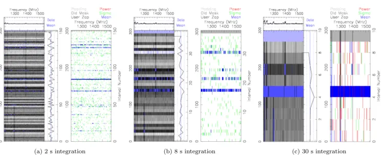
RFI masks created withPRESTO’srfifindfunction, for the
same file, are depicted in Figure11. The masks differ with
respect to the integration times used to create them. With
the plots in Figure11 we show that the RFI we injected,
although visible, is weak compared to the amplitude of the non-stationary baseline.
The default integration length of 30 s is most successful
at detecting the actual injected RFI (see Figure11c). The
two masks created with shorter integration times mostly flagged the maxima of the non-stationary baseline as
op-posed to the actual injected RFI (see Figure11aand
Fig-ure11b).
RFI was injected such that12 % of all the samples in
the data are affected. The 2 s mask in Figure 11a found
6.868 %of the 2 s intervals to be affected by RFI, the 8 s
mask in Figure11bfound6.887 %of the 8 s intervals to be
affected by RFI and the 30 s mask found that16.895 %of
the 30 s intervals are affected by RFI.
The focus of this section is on the real-time detection and mitigation of RFI, hence the decision to investigate the effectiveness of an RFI mask integrated over a few seconds when applied to the synthetic filterbank files. The results of
which can be seen in Figure12.
The RFI detection and masking routine available in
PRESTO had on average little to no effect on both the sen-sitivity and the number of false positives detected per true positive except for the non-stationary 3 with RFI case where
the sensitivity was increased from53 % to73 % when the
mask was applied. Greater insight on the effect of applying
the RFI detection and mitigation routine inPRESTOto files
containing weak RFI can be gained by comparing the results
of pipelines A-D to those of pipelines E-H in Figure14.
4.5 Variation of detection with signal significance The detection significance which pulsars embedded in dif-ferent noise processes were detected at by the default search
(a) No RFI (b) RFI
Figure 7.The performance ofSIGPROCandPRESTOfor processing files which contain either stationary noise or non-stationary noise with varying amplitudes (i.e. different values forh): (a) without RFI (see experiments 1 and 2 in Table2); (b) with RFI (see experiments 3 and 4 in Table2). (SIGPROCpipeline: default baseline subtraction→default red-noise removal.PRESTOpipeline: RFI mask→baseline not subtracted→default red-noise removal.)
Figure 8. The power spectrum density for different noise pro-cesses.
pipelines of SIGPROC andPRESTO are depicted in Figure13
with the colours being representative of the following: (a) Green square: an injected pulsar was detected (the
de-tection significance is printed in the square),
(b) Orange square: an injected pulsar is amongst the de-tected signals but is not considered a candidate because its detection significance is not above the default thresh-old value,
(c) Red square: signifies that an injected pulsar was missed, (d) Grey square: signifies that an injected pulsar was de-tected but is not considered a candidate because it has an abnormally high detection significance.
Each box in Figure 13 show a single instantiation of a
pulsar/non-stationary baseline pair that was searched by bothSIGPROCandPRESTO.
The left hand side of both matrices in Figure 13 are
populated with detections, whereas the right hand sides are predominantly populated with misses. Hence, long-period pulsars embedded in non-stationary noise processes across a range of correlation lengths are missed by both the default
SIGPROCandPRESTOpulsar search pipelines.
The detection significance at which pulsars with periods greater than 50 ms are detected decreases as the correlation length of the non-stationary noise shortens, whereas the de-tection significance of fast-period pulsars are unaffected by the correlation length of the non-stationary noise.
The results in Figure13portray single-trials for
near-threshold signals which are very sensitive to the noise real-isation used. To help understand the average and variance associated with the detection significance of these signals, we injected a pulsar with a period of 0.126 s in an ensemble of 20 noise realisations each with the same correlation length
of 1 s and amplitudeh=0.4 (see Equation 2). This
addi-tional experiment showed that the average SNR at which
the pulsar was detected inSIGPROCis 9 with a standard
de-viation of 1.45 compared to the SNR of 12.1 at which the pulsar is detected when embedded in stationary Gaussian noise. Similarly, the average Gaussian significance of the
de-tected pulsar inPRESTOis 6.621 with a standard deviation of
1.14 compared to the stationary Gaussian noise case of 7.7. Consequently, the results for this particular combination of
period and correlation length that are plotted in Figure13,
Figure14, Figure 15and Figure16would show very little
variability had there been more realisations of the same ex-periments. Multiple repetitions of this experiment over all combinations is extremely time costly and has not been at-tempted here. We have however computed similar standard
(a)SIGPROC (b)PRESTO
Figure 9.The performance of the red-noise mitigation methods available in (a)SIGPROCand (b)PRESTOfor processing files which contain either stationary noise (see experiment 1 in Table2) or non-stationary noise (see experiment 2 in Table2). No RFI were present in the files analysed. (SIGPROCpipeline: baseline intact→red-noise removal methods.PRESTOpipeline: RFI mask→baseline not subtracted→ red-noise removal method.)
(a)SIGPROC (b)PRESTO
Figure 10.The performance of the time-domain baseline normalisation methods available in (a)SIGPROCand (b)PRESTOfor processing files which contain non-stationary noise (see experiment 2 in Table2). No RFI was present in the files analysed. (SIGPROC pipeline: three time-domain baseline normalisation methods→default red-noise removal.PRESTOpipeline: No RFI mask→baseline normalisation method→no red-noise removal.)
deviations for other combinations of period and length scale
(e.g periods of 5 s, 0.01 s and 0.002 s, andλs of 1 s, 0.01 s
and 100 s), using small numbers of realizations (5 to 20). We find that the standard deviation in the experiments with no injected RFI remains similar to the measurements above, whereas the cases with RFI show increased variance, with
measured standard deviations of between 2 and 3. Although this will have an effect on a case by case basis, the overall statistical picture can be interpreted.
It is evident from Figure13aand Figure13b that the
pul-(a) 2 s integration (b) 8 s integration (c) 30 s integration
Figure 11.RFI masks created withPRESTO’srfifindfunction. The plots are for the same file but created with different integration times. The-timesigthreshold was set to three and the-freqsigthreshold was set to eight for therfifindfunction.
Figure 12.The efficacy of the RFI detection and masking rou-tine in PRESTO when processing files which contain either non-stationary noise (see experiment 2 in Table2) or non-stationary noise with weak RFI (see experiment 4 in Table 2). (PRESTO
pipeline: RFI Mask Yes/No→baseline intact→default red-noise removal.)
sars of various periods embedded in different non-stationary
noise processes compared toSIGPROC.
4.6 Sensitivity postcard plots of all the pipelines used to process files with PRESTO
The sensitivity plots for all the search pipelines explored in
PRESTO(see Table5) are depicted in Figure14.
None of the pipelines inPRESTOare able to detect all the
pulsars embedded in the different noise processes. Moreover, most of the pipelines miss the long-period pulsars. The
addi-tion of weak RFI, in general, does not alterPRESTO’s ability
to find pulsars.
Pipelines A, C, E and G in Figure 14 contain
detec-tions with Gaussian significances well in excess of the ex-pected maximum Gaussian significance. We do not consider these outliers as true detections. However, do note that these pipelines all have one thing in common and that is they do not whiten the spectrum.
The only difference between pipelines A to D and E to
H is the application of the RFI masking routine inPRESTO.
From the results it appears that the RFI routine attenuates the Gaussian significance of short period pulsars below the detection threshold both in the presence and absence of RFI. From these plots it is evident that running a moving average filter to normalise the time-domain data results in improved sensitivity, for example compare pipeline E with G and pipeline F with H. Note, when the moving average filter is applied in conjunction with the red-noise
suppres-sion method (see pipeline H in Figure14) then more
long-period pulsars embedded in non-stationary noise processes with long correlation lengths are detected compared to when only the moving average filter is applied (see pipeline F in
Figure14).
The pulsar search pipeline D inPRESTO (No RFI mask
→MA filter→red noise mitigation) yields the best results
amongst all the set-ups both in the presence and absence of RFI.
(a)SIGPROC
(b)PRESTO
Figure 13.The detection significance (values in black) at which 15 pulsars with different periods were detected (green squares) in files containing non-stationary noise processes with a relative amplitude ofh=0.4and five different correlation lengths (see experiment 5 in Table2). Each box represents a single instantiation of a pulsar/non-stationary baseline pair that was searched by bothSIGPROC and
PRESTO. The red squares represent missed pulsars and the orange squares represent detected pulsars with detection significances below the default threshold levels. (a) The results for files processed with the default pipeline inSIGPROC; (b) The results for files processed with the default pipeline inPRESTO.
4.7 Sensitivity postcard plots of all the pipelines used to process files with SIGPROC
The sensitivity plots for all the search pipelines explored in
SIGPROC (see Table4) are depicted in Figure 15 and
Fig-ure16.
Note, the pulsar with period 0.002218 s is detected
be-low the detection threshold (see orange squares in Figures15
and16) by almost all of the pipeline configurations in
SIG-PROCwhen RFI is present despite the other millisecond
pul-sars being detected. This pulsar is missed due to the in-creased variance of the SNR associated with the presence of
RFI as explored and explained in section§4.5.
It is apparent from pipelines D and H in Figure15and
pipeline L in Figure 16that not normalising the spectrum
results in a lot of pulsars being missed. Furthermore, mostly the long-period pulsars are regularly missed irrespective of
the pipeline used inSIGPROC.
Overall PRESTO’s performance across all the pipelines
is more consistent when compared the pipelines inSIGPROC.
5 DISCUSSION
With the advent of instruments like the Square Kilometre Array, real-time processing will become essential. Therefore, it is crucial that the pipeline employed to do this processing is optimal from the start. The purpose of the analysis in this paper was to investigate what improvements to current pulsar search pipelines are necessary before embarking on the development of a new real-time processing pipeline that is adept at dealing with the demands posed by this new era of pulsar astronomy.
This analysis demonstrated that non-stationary Gaus-sian noise processes with different correlation lengths lead to an increase in the number of false detections per true pulsar detection because of the static threshold applied in the power spectrum to distinguish between possible pulsar candidates and noise, i.e. non-stationary Gaussian noise is partly to blame for the so called ’crisis’ in candidate selec-tion (Lyon et al. 2016). In order to reduce the high number
of false positives, SIGPROC as well asPRESTO employ
spec-trum whitening methods. Our analysis has revealed how these methods decrease the number of false positives per
No RFI injected RFI injected (experiment 5 withh=0.4) (experiment 6 withh=0.4)
A B C D E F G H
Figure 14.The Gaussian significance at which pulsars were detected (green squares) after files containing them (see experiments 5 and 6 in Table2) were processed by eight different pipelines inPRESTO. The red squares represent missed pulsars, the orange squares represent detected pulsars with Gaussian significances below the default threshold level of 2 and the grey squares represent detected pulsars with Guassian significances above the average maximum Gaussian significance of 15.
true positive at the cost of a loss in sensitivity and detection significance to long-period pulsars.
The spectrum whitening techniques assessed in this analysis suppress the power in the lower frequencies to con-form to the power levels of the higher frequencies. Conse-quently, the spectral power of real signals from slowly rotat-ing pulsars is attenuated along with the noise. This analysis serves as evidence that there is room for improvement in the effectiveness of the current spectrum whitening methods. In-stead of forcing the spectrum to be uniform in the lower fre-quencies, the solution should rather be to accurately model the noise both in the spectral and in the time domain. In
fact we have shown that applying a 10 s moving average filter in the time domain resulted in a greater number of detections of long period pulsars. Consequently, leveraging moving averages on streaming data can help meet future real-time processing requirements whilst increasing surveys’ sensitivity to long period pulsars.
As we discussed earlier, the results presented in Fig-ure 13, Figure 14, Figure15 and Figure 16, are based on single realizations of period-length scale combinations. How-ever, we have sampled the standard deviation of the signifi-cance of these detections for several cases, and we conclude that although the picture may change for different
realiza-No RFI injected RFI injected Experiment 5 withh=0.4 Experiment 6 withh=0.4
A B C D E F G H
Figure 15.The SNR at which pulsars were detected after files containing them (see experiments 5 and 6 in Table2) were processed by eight different pipelines inSIGPROC. The red squares represent missed pulsars, the orange squares represent detected pulsars with SNRs below the default threshold level of 8 and the grey squares represent detected pulsars with SNRs above the average maximum SNR of 15.
tions and different initial S/N values of the injected pulsars, the areas in the plots which are most affected remain the same.
In this analysis we dedispersed all the files at the same
DM as what we injected the pulsars at (DM = 68 pc cm−3).
However, a subset of the files we dedispersed at four
ad-ditional DM values, namely 0, 20, 150 and 300 pc cm−3.
Dedispersing the files at these four additional DMs allowed us to confirm that the number of false positives detected by the pulsar search pipelines for the files containing both non-stationary noise and RFI are greatest when the filter-bank files are not dedispersed and decreases as one moves
away from 0 DM. However, the number of false positives detected by the pulsar search pipelines is very similar for the five DMs used to dedisperse the data. Consequently, the number of false positives detected for files containing only non-stationary noise is similar irrespective of the DM used to dedisperse the data.
In this analysis it was demonstrated that the RFI
de-tection algorithm inPRESTOis very sensitive to the interplay
between integration length over which the statistics of the filterbank files are computed and the rejection thresholds both in time and frequency of said statistics. For off-line processing this interplay can be fine tuned so that most RFI
No RFI injected RFI injected
I
J
K
L
Figure 16.The SNR at which pulsars were detected after files containing them (see experiments 5 and 6 in Table2) were processed by four additional pipelines inSIGPROC. The red squares represent missed pulsars, the orange squares represent detected pulsars with SNRs below the default threshold level of 8 and the grey squares represent detected pulsars with SNRs above the average maximum SNR of 15.
at different brightness levels can be detected and masked. However, for the real-time detection of RFI this exploration of parameter space is not always possible because of the time constraint as well as the dynamic nature of the RFI environment.
There are a multitude of modules each placed strate-gically throughout current pulsar search pipelines for de-tecting different sources of RFI. Most of these RFI detec-tion algorithms are largely amplitude-based and are there-fore very sensitive to non-stationary baselines. Consequently, data which contain no RFI but which have higher than av-erage mean and standard deviation are flagged as RFI. This analysis demonstrated that by flagging and replacing blocks of non-stationary data which contain no RFI or weak RFI may result in short period pulsars being attenuated below the detection threshold. Hence, there is a need for algorithms that can simultaneously normalise a non-stationary baseline and excise RFI signals superposed on said baseline without compromising the data that is not affected.
6 CONCLUSION
This paper gives a unified view of a typical pulsar search system. Moreover, it delves into the particulars of the al-gorithms available in the pulsar search software packages
SIGPROCandPRESTOfor spectrum whitening.
This analysis accords with the Lazarus et al. (2015)
PALFA sensitivity analysis that non-stationary noise and weak RFI leads to an increase in the number of false posi-tives and lower sensitivity for long period pulsars. These two effects have resulted in overestimates of survey production.
The severe degradation of the detection significance is partly due to frequency dependent noise and partly due ot
the attenuating nature of the spectrum whitening algorithms implemented in pulsar search software. Both these effects serve as explanation for why so many detectable long period normal pulsars are missed by pulsar search pipelines.
The analysis revealed that an increase in sensitivity was achieved when the data were de-trended with a moving aver-age filter with a window size larger than the slowest pulsar. However, it should be noted that the efficacy of the filter is dependent on the filter window size relative to the correla-tion length of the non-stacorrela-tionary noise process.
Following from the results of this paper it is now fea-sible to investigate methods for normalising a varying base-line as well as addressing the question of how to decouple the red noise from the signal without attenuating the de-tection significance. The effectiveness of these methods can be determined by applying them to the files created for this sensitivity analysis and then re-processing the normalised and modified files with the same pulsar search pipelines.
ACKNOWLEDGEMENTS
The authors wish to thank Paul Brook, Marisa Geyer, Jayanth Chennamangalam and Chris Williams for useful discussions. Additionally, the authors would like to thank Sean Passmoor, Lindsay Magnus and Justin Jonas at SKA South Africa for supplying the necessary RFI information required for this analysis. E. van Heerden would like to thank Bernard van Heerden for editorial revisions and ac-knowledges with gratitude the Commonwealth Scholarship Commission in the UK for providing financial support for this work. Finally, the authors would like to thank Scott Ransom, for useful comments that have helped improve the manuscript significantly.
REFERENCES
Antoniadis J., 2014, Multi-wavelength studies of pulsars and their companions. Springer
Barr E., 2013, Peasoup,https://github.com/ewanbarr/peasoup Bates S., Lorimer D., Rane A., Swiggum J., 2014, Monthly
No-tices of the Royal Astronomical Society, p. stu157
Burgay M., et al., 2006, Monthly Notices of the Royal Astronom-ical Society, 368, 283
Cordes J. M., et al., 2006a, The Astrophysical Journal, 637, 446 Cordes J. M., et al., 2006b, The Astrophysical Journal, 637, 446 Demorest P., Pennucci T., Ransom S., Roberts M., Hessels J.,
2010, Nature, 467, 1081
Hessels J. W., Ransom S. M., Stairs I. H., Freire P. C., Kaspi V. M., Camilo F., 2006, Science, 311, 1901
Hobbs G., Manchester R., Teoh A., Hobbs M., 2004, in Young Neutron Stars and Their Environments. p. 139
Johnston S., Lyne A., Manchester R., Kniffen D., D’amico N., Lim J., Ashworth M., 1992, Monthly Notices of the Royal Astronomical Society, 255, 401
Keith M., 2007, PhD thesis, University of Manchester Lazarus P., et al., 2015, The Astrophysical Journal, 812, 81 Levin L., et al., 2013, Monthly Notices of the Royal Astronomical
Society, p. stt1103
Lorimer D., 2001, Technical report, SIGPROC-v1. 0:(Pulsar) Sig-nal Processing Programs. Arecibo Technical Memo
Lorimer D. R., 2011, in , High-Energy Emission from Pulsars and their Systems. Springer, pp 21–36
Lorimer D. R., Kramer M., 2005, Handbook of pulsar astronomy. Vol. 4, Cambridge University Press
Lorimer D., et al., 1998, Astronomy and Astrophysics Supplement Series, 128, 541
Lorimer D., et al., 2006, Monthly Notices of the Royal Astronom-ical Society, 372, 777
Lyne A., Graham-Smith F., 2012, Pulsar astronomy. No. 48, Cam-bridge University Press
Lyon R., Stappers B., Cooper S., Brooke J., Knowles J., 2016, Monthly Notices of the Royal Astronomical Society, 459, 1104 Manchester R., Lyne A., Robinson C., D’Amico N., Bailes M.,
Lim J., 1991, Nature, 352, 219
Manchester R., et al., 1996, Monthly Notices of the Royal Astro-nomical Society, 279, 1235
Manchester R., et al., 2001, Monthly Notices of the Royal Astro-nomical Society, 328, 17
Nice D., Fruchter A., Taylor J., 1995, The Astrophysical Journal, 449, 156
Rane A., Lorimer D., Bates S., McMann N., McLaughlin M., Ra-jwade K., 2016, Monthly Notices of the Royal Astronomical Society, 455, 2207
Ransom S. M., 2001, PhD thesis, Harvard University Cambridge, Massachusetts
Ransom S., 2011, Astrophysics Source Code Library, 1, 07017 Ransom S. M., Eikenberry S. S., Middleditch J., 2002, The
As-tronomical Journal, 124, 1788 Rasmussen C. E., Williams C. K. I., 2006
Regulations R., 2008, Radiocommunication Sector. ITU-R. Geneva
Seward F., Harnden Jr F., 1982, The Astrophysical Journal, 256, L45
Stovall K., et al., 2014, The Astrophysical Journal, 791, 67 Swiggum J., et al., 2014, The Astrophysical Journal, 787, 137 van Heerden E., Karastergiou A., Roberts S., Smirnov O., 2014, in
General Assembly and Scientific Symposium (URSI GASS), 2014 XXXIth URSI. pp 1–4
This paper has been typeset from a TEX/LATEX file prepared by the author.