Robust Deep Learning in the Open World with Lifelong Learning and Representation Learning

(1)

Robust Deep Learning in the Open World with

Lifelong Learning and Representation Learning

by

Kibok Lee

A dissertation submitted in partial fulfillment

of the requirements for the degree of

Doctor of Philosophy

(Computer Science and Engineering)

in the University of Michigan

2020

Doctoral Committee:

Associate Professor Honglak Lee, Chair

Assistant Professor David Fouhey

Professor Alfred O. Hero, III

Assistant Professor Justin Johnson

(2)

Kibok Lee [email protected]

ORCID iD: 0000-0001-6995-7327

(3)

ACKNOWLEDGEMENTS

First of all, I would like to express my sincere gratitude to my advisor, Professor Honglak Lee, for his guidance and support throughout my graduate studies. It was an honor and privilege to have him as a mentor. All my works presented in this dissertation would not have been possible without his insightful advice. I would also like to thank Professor Jinwoo Shin and Kimin Lee from KAIST for their continuous collaboration with me. More than half of my publications have been written through discussion with them.

I would like to extend my appreciation to my dissertation committee members, Pro-fessor David Fouhey, ProPro-fessor Alfred O. Hero III, and ProPro-fessor Justin Johnson. They provided valuable feedback on this dissertation.

I would like to thank all my former and current labmates for their valuable discussions and warm friendship: Scott Reed, Yuting Zhang, Wenling Shang, Junhyuk Oh, Ruben Villegas, Xinchen Yan, Ye Liu, Seunghoon Hong, Lajanugen Logeswaran, Rui Zhang, Sungryull Sohn, Jongwook Choi, Yijie Guo, Yunseok Yang, Wilka Carvalho, Anthony Liu, and Thomas Huang.

Many thanks to all my collaborators in academia and industry: Professor Anna Gilbert, Yi Zhang, Kyle Min, and Yian Zhu from UMich, Professor Bo Li from UIUC, Sukmin Yun from KAIST, Woojoo Sim from Samsung, Ersin Yumer, Raquel Urtasun, and Zhuoyuan Chen from Uber ATG, and Kihyuk Sohn and Chun-Liang Li from Google Cloud AI.

I am grateful to have had the opportunity to work on research projects at Uber ATG as a research intern, which allowed me to experience conducting research from an industrial perspective.

I would like to express my deepest gratitude to my family for their endless love and support. My parents and brother have always been a source of comfort and hope in difficult times. Your presence has been a great pleasure and encouragement to me.

Lastly, I gratefully acknowledge the financial support from Kwanjeong Educational Foundation Scholarship, Samsung Electronics, NSF CAREER IIS-1453651, ONR N00014-16-1-2928, and DARPA Explainable AI (XAI) program #313498.

(4)

LIST OF FIGURES

Figure

2.1 An illustration of our proposed hierarchical novelty detection task. In contrast to prior novelty detection works, we aim to find the most specific class label of a novel data on the taxonomy built with known classes. . . 10 2.2 Illustration of two proposed approaches. In the top-down method,

clas-sification starts from the root class, and propagates to one of its children until the prediction arrives at a known leaf class (blue) or stops if the pre-diction is not confident, which means that the prepre-diction is a novel class whose closest super class is the predicted class. In the flatten method, we add a virtual novel class (red) under each super class as a representative of all novel classes, and then flatten the structure for classification. . . 13 2.3 Illustration of strategies to train novel class scores in flatten methods. (a)

shows the training images in the taxonomy. (b) shows relabeling strategy. Some training images are relabeled to super classes in a bottom-up man-ner. (c–d) shows leave-one-out (LOO) strategy. To learn a novel class score under a super class, one of its children is temporarily removed such that its descendant known leaf classes are treated as novel during training. 17 2.4 Qualitative results of hierarchical novelty detection on ImageNet. “GT”

is the closest known ancestor of the novel class, which is the expected pre-diction, “DARTS” is the baseline method proposed inDeng et al.(2012) where we modify the method for our purpose, and the others are our pro-posed methods. “ε” is the distance between the prediction and GT, “A”

indicates whether the prediction is an ancestor of GT, and “Word” is the English word of the predicted label. Dashed edges represent multi-hop connection, where the number indicates the number of edges between classes. If the prediction is on a super class (marked with * and rounded), then the test image is classified as a novel class whose closest class in the taxonomy is the super class. . . 21 2.5 Known-novel class accuracy curves obtained by varying the novel class

score bias on ImageNet, AwA2, and CUB. In most regions, our proposed methods outperform the baseline method. . . 22

(8)

2.6 Seen-unseen class accuracy curves of the best combined models obtained by varying the unseen class score bias on AwA1, AwA2, and CUB. “Path” is the hierarchical embedding proposed inAkata et al.(2015), and “TD” is the embedding of the multiple softmax probability vector obtained from the proposed top-down method. In most regions, TD outperforms Path. . . 25 3.1 We propose to leverage a large stream of unlabeled data in the wild for

class-incremental learning. At each stage, a confidence-based sampling strategy is applied to build an external dataset. Specifically, some of un-labeled data are sampled based on the prediction of the model learned in the previous stageP for alleviating catastrophic forgetting, and some of

them are randomly sampled for confidence calibration. Under the combi-nation of the labeled training dataset and the unlabeled external dataset, a teacher modelC first learns the current task, and then the new modelM

learns both the previous and current tasks by distilling the knowledge of

P,C, and their ensembleQ. . . 27

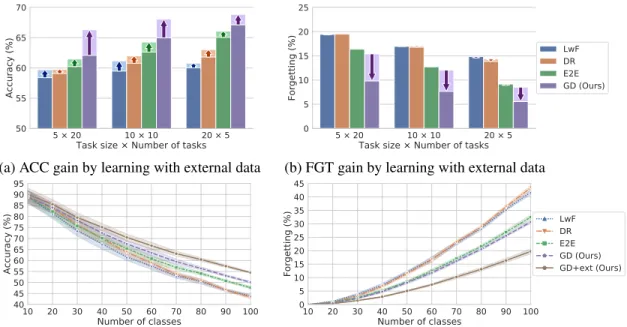
3.2 Experimental results on CIFAR-100. (a,b) Arrows show the performance gain in the average incremental accuracy (ACC) and average forgetting (FGT) by learning with unlabeled data, respectively. (c,d) Curves show ACC and FGT with respect to the number of trained classes when the task size is 10. We report the average performance of ten trials. . . 41 4.1 (a) Examples of randomized inputs (color values in each channel are

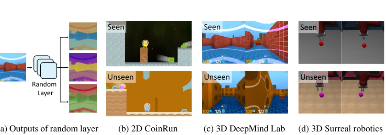
nor-malized for visualization) generated by re-initializing the parameters of a random layer. Examples of seen and unseen environments on (b) Coin-Run, (c) DeepMind Lab, and (d) Surreal robotics control. . . 45 4.2 Samples of dogs vs. cats dataset. The training set consists of bright dogs

and dark cats, whereas the test set consists of dark dogs and bright cats. . 49 4.3 (a) We collect multiple episodes from various environments by human

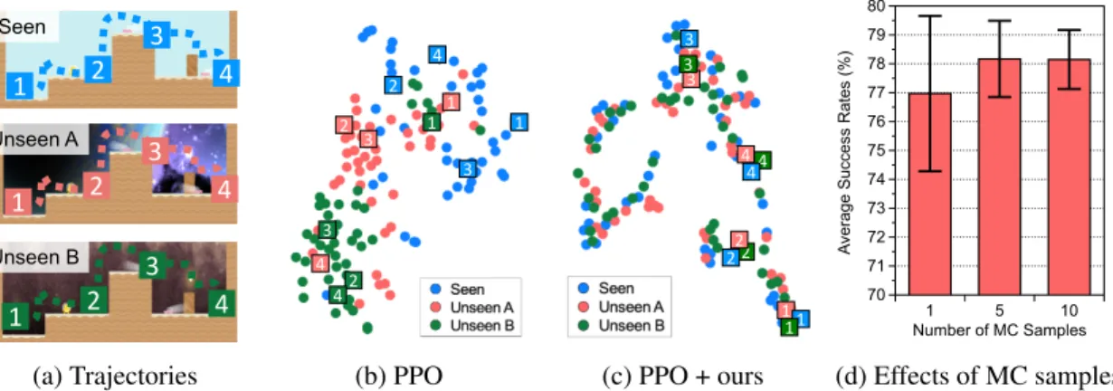
demonstrators and visualize the hidden representation of trained agents optimized by (b) PPO and (c) PPO + ours constructed by t-SNE, where the colors of points indicate the environments of the corresponding ob-servations. (d) Average success rates for varying number of MC samples. 53 4.4 Visualization of activation maps via Grad-CAM in seen and unseen

en-vironments in the small-scale CoinRun. Images are aligned with similar states from various episodes for comparison. . . 54 4.5 The performances of trained agents in unseen environments under (a)

large-scale CoinRun, (b) DeepMind Lab and (c) Surreal robotics control. The solid/dashed lines and shaded regions represent the mean and stan-dard deviation, respectively. . . 55 5.1 Comparison of performance gains by applying i-MixUp to N-pair

con-trastive learning with different model sizes and number of training epochs. The pretext and downstream tasks share the same dataset. While training more than 1000 epochs does not improve the performance of contrastive learning,i-MixUp benefits from longer training. . . 68

(9)

5.2 Comparison of contrastive learning andi-MixUp with ResNet-50 on

CIFAR-10 and CIFAR-100 with the different training dataset size. The pretext and downstream shares training dataset. The absolute performance gain byi

-MixUp in contrastive learning does not decrease when the training dataset

size increases. . . 69

5.3 t-SNE visualization of embeddings trained by contrastive learning andi -MixUp with ResNet-50 on CIFAR-10. (a,b): Classes are well-clustered in both cases when applied to CIFAR-10. (c,d): When models are trans-ferred to CIFAR-100, classes are more clustered fori-MixUp than con-trastive learning, as highlighted in dashed boxes. We show 10 classes for a better visualization. . . 70

A.1 Qualitative results of hierarchical novelty detection on ImageNet. . . 82

A.9 Sub-taxonomies of the hierarchical novelty detection results of a known leaf class “Cardigan Welsh corgi.” (Best viewed when zoomed in on a screen.) . . . 90

A.10 Sub-taxonomies of the hierarchical novelty detection results of a known leaf class “digital clock.” (Best viewed when zoomed in on a screen.) . . 91

A.11 Sub-taxonomies of the hierarchical novelty detection results of novel classes whose closest class in the taxonomy is “foxhound.” (Best viewed when zoomed in on a screen.) . . . 91

A.12 Sub-taxonomies of the hierarchical novelty detection results of novel classes whose closest class in the taxonomy is “wildcat.” (Best viewed when zoomed in on a screen.) . . . 91

A.13 Sub-taxonomies of the hierarchical novelty detection results of novel classes whose closest class in the taxonomy is “shark.” (Best viewed when zoomed in on a screen.) . . . 92

A.14 Sub-taxonomies of the hierarchical novelty detection results of novel classes whose closest class in the taxonomy is “frozen dessert.” (Best viewed when zoomed in on a screen.) . . . 92

A.15 An example of taxonomy and the correspondingty values. . . 93

A.16 Taxonomy of AwA built with the split proposed in (Xian et al., 2017) (top) and the split we propose for balanced taxonomy (bottom). Taxon-omy is built with known leaf classes (blue) by finding their super classes (white), and then novel classes (red) are attached for visualization. . . 93

(10)

A.17 Seen-unseen class accuracy curves of the best combined models obtained by varying the unseen class score bias on AwA1 and AwA2, with the split of imbalanced taxonomy and that of balanced taxonomy. “Path” is the hierarchical embedding proposed in (Akata et al.,2015), and “TD” is the embedding of the multiple softmax probability vector obtained from the proposed top-down method. We remark that if the dataset has a balanced taxonomy, the overall performance can be improved. . . 95 B.1 An illustration of how a model Mlearns with global distillation (GD).

For GD, three reference models are used: P is the previous model,C is

the teacher for the current task, andQis an ensemble of them. . . 96

B.2 Experimental results on CIFAR-100 and ImageNet when the task size is 10. We report ACC and FGT with respect to the OOD ratio averaged over ten trials for CIFAR-100 and nine trials for ImageNet. . . 98 B.3 Experimental results on ImageNet when the task size is 10. We report

ACC and FGT with respect to the hierarchical distance between the train-ing dataset and unlabeled data stream averaged over nine trials. . . 98 B.4 Experimental results on ImageNet. Arrows show the performance gain in

ACC and FGT by learning with unlabeled data, respectively. We report the average performance of nine trials. . . 100 B.5 Experimental results on CIFAR-100 when the task size is 5. We report

ACC and FGT with respect to the number of trained classes averaged over ten trials. . . 100 B.6 Experimental results on CIFAR-100 when the task size is 20. We report

ACC and FGT with respect to the number of trained classes averaged over ten trials. . . 100 B.7 Experimental results on ImageNet when the task size is 5. We report ACC

and FGT with respect to the number of trained classes averaged over nine trials. . . 101 B.8 Experimental results on ImageNet when the task size is 10. We report

ACC and FGT with respect to the number of trained classes averaged over nine trials. . . 101 B.9 Experimental results on ImageNet when the task size is 20. We report

ACC and FGT with respect to the number of trained classes averaged over nine trials. . . 101 C.1 Learning curves on (a) small-scale, (b) large-scale CoinRun and (c)

Deep-Mind Lab. The solid line and shaded regions represent the mean and standard deviation, respectively, across three runs. . . 102 C.2 The performance in unseen environments in small-scale CoinRun. The

solid/dashed line and shaded regions represent the mean and standard deviation, respectively, across three runs. . . 103 C.3 Network architectures with random networks in various locations. Only

convolutional layers and the last fully connected layer are displayed for conciseness. . . 105

(11)

C.4 The performance of random networks in various locations in the network architecture on (a) seen and (b) unseen environments in large-scale Coin-Run. We show the mean performances averaged over three different runs, and shaded regions represent the standard deviation. . . 106 C.5 Examples of seen and unseen environments in small-scale CoinRun. . . . 106 C.6 Examples of seen and unseen environments in large-scale CoinRun. . . . 107 C.7 The top-down view of the trained map layouts. . . 108 C.8 (a) An illustration of network architectures for the Surreal robotics

con-trol experiment, and learning curves with (b) regularization and (c) data augmentation techniques. The solid line and shaded regions represent the mean and standard deviation, respectively, across three runs. . . 109 C.9 Examples of seen and unseen environments in the Surreal robot

manipu-lation. . . 110 C.10 Performances of trained agents in seen and unseen environments under

(a/b) CartPole and (c/d) Hopper. The solid/dashed lines and shaded re-gions represent the mean and standard deviation, respectively. . . 111 C.11 (a) Modified CoinRun with good and bad coins. The performances on

(b) seen and (c) unseen environments. The solid line and shaded regions represent the mean and standard deviation, respectively, across three runs. (d) Average success rates on large-scale CoinRun for varying the fraction of clean samples during training. Noe thatα = 1 corresponds to vanilla

PPO agents. . . 112 C.12 Visualization of the hidden representation of trained agents optimized by

(a) PPO, (b) PPO + L2, (c) PPO + BN, (d) PPO + DO, (e) PPO + CO, (f) PPO + GR, (g) PPO + IV, (h) PPO + CJ, and (I) PPO + ours using t-SNE. The point colors indicate the environments of the corresponding observations. . . 113

(12)

LIST OF TABLES

Table

2.1 Hierarchical novelty detection results on ImageNet, AwA2, and CUB. For a fair comparison, 50% of known class accuracy is guaranteed by adding a bias to all novel class scores (logits). The AUC is obtained by vary-ing the bias. Known-novel class accuracy curve is shown in Figure 2.5. Values in bold indicate the best performance. . . 20 2.2 ZSL and GZSL performance of semantic embedding models and their

combinations on AwA1, AwA2, and CUB. “Att” stands for continuous attributes labeled by human, “Word” stands for word embedding trained with the GloVe objective (Pennington et al., 2014), and “Hier” stands for the hierarchical embedding, where “Path” is proposed inAkata et al.

(2015), and “TD” is output of the proposed top-down method. “Unseen” is the accuracy when only unseen classes are tested, and “AUC” is the area under the seen-unseen curve where the unseen class score bias is varied for computation. The curve used to obtain AUC is shown in Figure 2.6. Values in bold indicate the best performance among the combined mod-els. . . 24 3.1 Comparison of methods on CIFAR-100 and ImageNet. We report the

mean and standard deviation of ten trials for CIFAR-100 and nine trials for ImageNet with different random seeds in %. ↑(↓) indicates that the

higher (lower) number is the better. . . 40 3.2 Comparison of models learned with different reference models on

CIFAR-100 when the task size is 10. “P,” “C,” and “Q” stand for the previous

model, the teacher for the current task, and their ensemble model, respec-tively. . . 41 3.3 Comparison of models learned with a different teacher for the current

task C on CIFAR-100 when the task size is 10. For “cls,” C is not

trained but the model learns by optimizing the learning objective of C

directly. The model learns with the proposed 3-step learning for “dst.”

The confidence loss is added to the learning objective for C for “cnf.”

(13)

3.4 Comparison of different balanced learning strategies on CIFAR-100 when the task size is 10. “DW,” “FT-DSet,” and “FT-DW” stand for training with data weighting in Eq. (3.10) for the entire training, fine-tuning with a training dataset balanced by removing data of the current task, and fine-tuning with data weighting, respectively. . . 42 3.5 Comparison of different external data sampling strategies on

CIFAR-100 when the task size is 10. “Prev” and “OOD” columns describe the sampling method for data of previous tasks and out-of-distribution data, where “Pred” and “Random” stand for sampling based on the prediction of the previous model P and random sampling, respectively. In

particu-lar, for when sampling OOD by “Pred,” we sample data minimizing the confidence lossLcnf. When only Prev or OOD is sampled, the number of sampled data is doubled for fair comparison. . . 43 4.1 Classification accuracy (%) on dogs vs. cats dataset. The results show the

mean and standard deviation averaged over three runs and the best result is indicated in bold. . . 49 4.2 Success rate (%) and cycle-consistency (%) after 100M timesteps in

small-scale CoinRun. The results show the mean and standard deviation aver-aged over three runs and the best results are indicated in bold. . . 52 4.3 Comparison with domain randomization. The results show the mean and

standard deviation averaged over three runs and the best results are indi-cated in bold. . . 56 5.1 Comparison of memory-free and memory-based contrastive learning

meth-ods andi-MixUp on them with ResNet-50 on CIFAR-10 and 100. We

re-port the mean and standard deviation of five trials with different random seeds in %. Equation number indicates the loss function of each method.

i-MixUp improves the accuracy on the downstream task regardless of the

data distribution shift between the pretext and downstream tasks. . . 67 5.2 Comparison of contrastive learning andi-MixUp with ResNet-50 on

CIFAR-10 and CIFAR-100 under different data augmentation methods: when 1) no data augmentation is available, 2) domain-agnostic data augmentation meth-ods are applied, and 3) domain-specific data augmentation methmeth-ods are applied. i-MixUp improves the performance of contrastive learning in all

cases. . . 71 5.3 Comparison of contrastive learning andi-MixUp on Speech Commands (

War-den,2018) and tabular datasets from UCI machine learning repository ( Asun-cion and Newman, 2007). i-MixUp improves the performance of

con-trastive learning on those non-image domains. . . 72 5.4 Comparison of MoCo v2 (Chen et al.,2020b) andi-MixUp with

ResNet-50 on ImageNet. . . 72 A.1 Hierarchical novelty detection results on CIFAR-100. For a fair

compar-ison, 50% of known class accuracy is guaranteed by adding a bias to all novel class scores (logits). The AUC is obtained by varying the bias. . . . 80

(14)

A.2 ZSL and GZSL performance of semantic embedding models and their combinations on AwA1 and AwA2 in the split of imbalanced taxonomy and that of balanced taxonomy. “Att” stands for continuous attributes labeled by human, “Word” stands for word embedding trained with the GloVe objective (Pennington et al.,2014), and “Hier” stands for the hier-archical embedding, where “Path” is proposed in (Akata et al.,2015), and “TD” is output of the proposed top-down method. “Unseen” is the accu-racy when only unseen classes are tested, and “AUC” is the area under the seen-unseen curve where the unseen class score bias is varied for compu-tation. The curve used to obtain AUC is shown in Figure A.17. Values in bold indicate the best performance among the combined models. . . 94 B.1 Comparison of methods on CIFAR-100 and ImageNet. We report the

mean and standard deviation of ten trials for CIFAR-100 and nine trials for ImageNet with different random seeds in %. ↑(↓) indicates that the

higher (lower) number is the better. . . 99 C.1 Robustness against FGSM attacks on training environments. The values

in parentheses represent the relative reductions from the clean samples. . . 104 C.2 Action set used in the DeepMind Lab experiment. The DeepMind Lab

native action set consists of seven discrete actions encoded in integers ([L,U] indicates the lower/upper bound of the possible values): 1) yaw (left/right) rotation by pixel [-512,512], 2) pitch (up/down) rotation by pixel [-512,512], 3) horizontal move [-1,1], 4) vertical move [-1,1], 5) fire [0,1], 6) jump [0,1], and 7) crouch [0,1]. . . 108 D.1 Comparison of N-pair contrastive learning, SimCLR, MoCo, andi-MixUp

andi-CutMix on them with ResNet-50 on CIFAR-10 and 100. We report

the mean and standard deviation of five trials with different random seeds in %.i-MixUp improves the accuracy on the downstream task regardless

of the data distribution shift between the pretext and downstream tasks.

i-CutMix shows a comparable performance withi-MixUp when the

pre-text and downstream datasets are the same, but it does not when the data distribution shift occurs. . . 118 D.2 Comparison of the N-pair self-supervised and supervised contrastive

learn-ing methods and i-MixUp on them with ResNet-50 on CIFAR-10 and

100. We also provide the performance of formulations proposed in prior works: SimCLR (Chen et al., 2020a) and supervised SimCLR (Khosla et al.,2020). i-MixUp improves the accuracy on the downstream task

re-gardless of the data distribution shift between the pretext and downstream tasks, except the case that the pretest task has smaller number of classes than that of the downstream task. The quality of representation depends on the pretext task in terms of the performance of transfer learning: self-supervised learning is better on CIFAR-10, while self-supervised learning is better on CIFAR-100. . . 119

(15)

D.3 Comparison of contrastive learning andi-MixUp with ResNet-50 on

CIFAR-10 and CIFAR-100 in terms of the Fréchet embedding distance (FED) between training and test data distribution on the embedding space, and training and test accuracy.↑(↓) indicates that the higher (lower) number is the

bet-ter. i-MixUp improves contrastive learning in all metrics, which shows

that i-MixUp is an effective regularization method for the pretext task,

(16)

LIST OF APPENDICES

Appendix

A. Supplementary Material of Chapter II . . . 77

B. Supplementary Material of Chapter III . . . 96

C. Supplementary Material of Chapter IV . . . 102

(17)

ABSTRACT

Deep neural networks have shown a superior performance in many learning problems by learning hierarchical latent representations from a large amount of labeled data. How-ever, the success of deep learning methods is under the closed-world assumption: no in-stances of new classes appear at test time. On the contrary, our world is open and dynamic, such that the closed-world assumption may not hold in many real applications. In other words, deep learning-based agents are not guaranteed to work in the open world, where instances of unknown and unseen classes are pervasive.

In this dissertation, we explore lifelong learning and representation learning to gen-eralize deep learning methods to the open world. Lifelong learning involves identifying novel classes and incrementally learning them without training from scratch, and represen-tation learning involves being robust to data distribution shifts. Specifically, we propose 1) hierarchical novelty detection for detecting and identifying novel classes, 2) continual learning with unlabeled data to overcome catastrophic forgetting when learning the novel classes, 3) network randomization for learning robust representations across visual domain shifts, and 4) domain-agnostic contrastive representation learning, which is robust to data distribution shifts.

The first part of this dissertation studies a cycle of lifelong learning. We divide it into two steps and present how we can achieve each step: first, we propose a new novelty detection and classification framework termed hierarchical novelty detection for detecting and identifying novel classes. Then, we show that unlabeled data easily obtainable in the open world are useful to avoid forgetting about the previously learned classes when learning novel classes. We propose a new knowledge distillation method and confidence-based sampling method to effectively leverage the unlabeled data.

The second part of this dissertation studies robust representation learning: first, we present a network randomization method to learn an invariant representation across visual changes, particularly effective in deep reinforcement learning. Then, we propose a domain-agnostic robust representation learning method by introducing vicinal risk minimization in contrastive representation learning, which consistently improves the quality of representa-tion and transferability across data distriburepresenta-tion shifts.

(18)

CHAPTER I

Introduction

1.1 Motivation

Deep learning is a class of machine learning algorithms that aims to learn hierarchical latent representations from high-dimensional raw data (Hinton and Salakhutdinov, 2006;

LeCun et al., 2015). The power of deep learning lies not only in eliminating the need for hand-crafted features, but also in boosting the performance of machine learning algorithms. Deep learning has been considered a core method to make progress toward artificial intel-ligence. Specifically, deep learning approaches have been successfully applied in many learning problems, such as visual recognition (Girshick et al.,2014;Simonyan and Zisser-man, 2015;He et al., 2016), speech recognition (Hinton et al., 2012;Graves et al.,2013), natural language processing (Mikolov et al.,2013;Pennington et al.,2014), and reinforce-ment learning (Mnih et al.,2015;Silver et al.,2017).

However, the success of deep learning methods is mostly under the closed-world as-sumption: training and test data are drawn from the same distribution, such that no in-stances of unknown or unseen classes appear at test time. On the contrary, many real-world problems do not satisfy this assumption as they lie in the open world. Therefore, the robust-ness of deep learning has been a serious concern regarding its practical applicability. To generalize deep learning methods to real-world applications, several research topics have been explored, including representation learning (Bengio et al., 2013;Chen et al., 2020a;

He et al.,2020), domain adaptation (Ganin and Lempitsky,2015;Ganin et al.,2016;Tobin et al.,2017), transfer learning (Donahue et al.,2014;Razavian et al.,2014;Yosinski et al.,

2014), out-of-distribution detection (Hendrycks and Gimpel, 2016; Lee et al., 2018b,c), adversarial robustness (Szegedy et al.,2014;Goodfellow et al.,2015;Nguyen et al.,2015), lifelong learning (Li and Hoiem, 2016; Kirkpatrick et al., 2017;Parisi et al., 2019), zero-shot learning (Rohrbach et al.,2011;Xian et al.,2017), and few-shot learning (Koch et al.,

(19)

2015; Santoro et al., 2016; Vinyals et al., 2016). In this dissertation, we study lifelong learning and representation learning in the open-world setting for successful deployment of deep learning methods to real-world applications.

Lifelong learning aims to continually learn over time by acquiring new knowledge from

a continuous stream of data while retaining previously learned knowledge (Thrun and Mitchell,1995;Silver et al.,2013;Hassabis et al.,2017;Chen and Liu,2018;Parisi et al.,

2019). Humans are innately motivated to continually learn to improve their knowledge and develop their skills throughout their lives. Similarly, in real-world applications, in-telligent agents are exposed to ever-changing environments, such that they are required to continually learn from their experiences to operate in new environments in their lifetime. For example, autonomous driving agents should interact with environments, such that they arrive at the destination without accident in any conditions. Lifelong learning enables the agents to deal with unexpected cases occurring in the real world. While most of the life-long learning works have focused on classification tasks (Li and Hoiem,2016;Kirkpatrick et al.,2017), lifelong learning has become successful with deep architectures in many dif-ferent machine learning tasks, including representation learning (Rao et al., 2019), object detection (Liu et al., 2020), natural language processing (Sun et al., 2020), reinforcement learning (Tessler et al.,2017;Schwarz et al.,2018), and robotics (Lesort et al.,2020).

Lifelong learning can be divided into two steps: first, the agents should detect and iden-tify “what to learn.” To achieve this, novelty or out-of-distribution detection (Manevitz and Yousef,2001;Pimentel et al.,2014;Hendrycks and Gimpel,2016;Lee et al.,2018b,c) can be considered, as it is a task to detect objects never seen before. Novelty detection has several interchangeable terms with subtle differences: anomaly detection, outlier de-tection, and out-of-distribution detection. Anomaly or outlier detection implicitly assumes that detected novelties should be rejected as they are abnormal (Pimentel et al., 2014). However, novelty or out-of-distribution detection aims to distinguish known and novel ob-jects, which could be from either unknown classes or unknown distribution. In lifelong learning, the goal of detection is to learn them, so novelty or out-of-distribution would be more appropriate. In particular, out-of-distribution (Hendrycks and Gimpel, 2016; Lee et al., 2018b,c) has recently gained increasing attention, as deep learning models are over-confident in their predictions, which are highly biased to in-distribution observed during training. However, novelty detection results are only the novelty of inputs, such that hu-man annotation is required before learning them. In other words, the conventional novelty detection is not directly applicable to lifelong learning.

(20)

classifi-cation framework termed hierarchical novelty detection to provide better identificlassifi-cation of the novel objects to the agents. More specifically, in hierarchical novelty detection, novel classes are expected to be classified as semantically the most relevant label, i.e., the clos-est class in the hierarchical taxonomy built with known classes. For example, if an agent knows dogs, cats, and birds, it infers the general characteristics of dogs and cats, which are categorized as mammals. Then, when the agent observes a bear, hierarchical novelty de-tection enables the agent to predict its label as novel mammal. In this way, the knowledge of the agent is more organized based on the similarity of objects, such that the agent is able to efficiently learn on top of its simplified representation.

Next, the agents should continually update their knowledge without forgetting previ-ously learned knowledge. Continual lifelong learning has been studied with different as-sumptions. Broadly speaking, there are three types of problems (van de Ven and Tolias,

2018): first, the goal of task-incremental learning (Li and Hoiem, 2016; Hou et al., 2018) is a kind of multitask learning, but tasks are sequentially given. In this problem, task boundaries are assumed to be clear and the agent receives information about the task at test time. Another is data- or domain-incremental learning (Kirkpatrick et al., 2017;Rusu et al., 2016b; Schwarz et al., 2018), where task identities are not available at test time. Instead, the output space is also fixed, such that the agent learns to generalize previously observed classes. Many robotics and reinforcement learning problems follow this assump-tion: for example, agents in video games (Bellemare et al., 2013; Cobbe et al., 2019) or 3D simulated environments (Beattie et al., 2016; Fan et al., 2018) have a predefined set of actions, but they can perform multiple tasks with the actions. Lastly, class-incremental learning (Rebuffi et al., 2017;Castro et al.,2018;Wu et al.,2018a;Lee et al.,2019a) does not assume explicit task boundaries, nor is the output space fixed.

In continual learning, deep learning agents easily forget about previously learned knowl-edge while acquiring new knowlknowl-edge, which is often referred to as catastrophic forget-ting (McCloskey and Cohen, 1989; French, 1999). There are two main streams of con-tinual learning methods to overcome catastrophic forgetting: model-based and data-based. Model-based approaches (Rusu et al., 2016b; Kirkpatrick et al., 2017; Lee et al., 2017;

Lopez-Paz et al., 2017; Zenke et al., 2017; Aljundi et al., 2018; Chaudhry et al., 2018;

Jung et al., 2018; Mallya et al., 2018; Nguyen et al., 2018; Ritter et al., 2018; Schwarz et al., 2018; Serra et al., 2018; Yoon et al., 2018) keep the knowledge of previous tasks by penalizing the change of parameters crucial for previous tasks, such that measuring the importance of parameters on previous tasks is important in these approaches. Data-based approaches (Li and Hoiem,2016;Rebuffi et al.,2017;Castro et al.,2018;Hou et al.,2018;

(21)

pre-vious tasks by knowledge distillation (Hinton et al.,2015), which minimizes the distance between the manifold of the latent space in the previous and new models. In contrast to model-based approaches, they require data to be fed to get features on the latent space. As the similarity between the previously and newly learned tasks is important to prevent catas-trophic forgetting, a small amount of memory is reserved to keep a coreset of data from previous tasks (Rebuffi et al., 2017; Castro et al., 2018; Nguyen et al., 2018; Lee et al.,

2019a), or a generative model is trained to replay data of previous tasks (Rannen et al.,

2017;Shin et al.,2017;Lesort et al.,2018;van de Ven and Tolias, 2018;Wu et al.,2018a) when training a new model.

Our second contribution in Chapter IIIis motivated by the fact that intelligent agents are exposed to streams of unlabeled data in the real world. To alleviate catastrophic forget-ting, we propose to leverage unlabeled data easily obtainable in the open world. However, learning with infinite amounts of unlabeled data is inefficient, and the learning objectives proposed in prior works are not capable of fully leveraging unlabeled data, as they are studied under the closed-world assumption. To this end, we propose a confidence-based sampling method and a new learning objective for continual learning, termed global dis-tillation. With hierarchical novelty detection and continual learning in the open world, intelligent agents grow closer to being successfully applied in real-world applications.

Representation learning is a fundamental problem of machine learning (Lee et al.,2007;

Bengio et al., 2013): it aims to extract useful information from data for deployment to other machine learning applications. Indeed, the performance of machine learning meth-ods heavily depends on the data representations. The success of deep learning is from the better quality of deeply learned features (Girshick et al., 2014; Razavian et al., 2014) compared with handcrafted ones, e.g., SIFT (Lowe, 1999) and HOG (Dalal and Triggs,

2005) in computer vision, and MFCC (Davis and Mermelstein, 1980) in speech process-ing. Deep representation learning has been studied in both supervised and unsupervised ways: a simple but effective way of supervised representation learning is to extract latent features from convolutional neural networks (Krizhevsky et al., 2012;He et al.,2015; Si-monyan and Zisserman, 2015;Szegedy et al.,2015;He et al.,2016;Szegedy et al., 2016) trained on large-scale datasets (Deng et al.,2009) in classification tasks. In particular, deep metric learning (Yi et al., 2014; Hoffer and Ailon, 2015; Sohn, 2016; Song et al., 2016) focuses more on learning distance metrics in a supervised way. Unsupervised representa-tion learning aims for learning representarepresenta-tions from unlabeled data by solving pretext tasks that are different from downstream tasks. It is often referred to as self-supervised learn-ing, as the learning problem of pretext tasks is based on self-supervision. Among many

(22)

self-supervised pretext tasks designed for representation learning, data reconstruction by autoencoding (Bengio et al., 2007;Vincent et al.,2010;Kingma and Welling,2014), clas-sifying individual instances (Dosovitskiy et al.,2014;Wu et al.,2018b;Chen et al.,2020a;

He et al., 2020), and clustering (Xie et al., 2016;Caron et al.,2018, 2019;Ji et al., 2019;

Asano et al.,2020;Yan et al.,2020) have been popular in recent literature.

However, deeply learned representations tend to overfit to training data distributions, such that the application of deep learning to the real world is challenging (Szegedy et al.,

2014;Goodfellow et al.,2015;Hendrycks and Gimpel, 2016;Lee et al., 2018b). Specifi-cally, domain generalization (Ganin and Lempitsky,2015;Ganin et al.,2016;Tobin et al.,

2017) and transfer learning (Donahue et al., 2014; Razavian et al., 2014; Yosinski et al.,

2014) aim to generalize learned representations to different domains and tasks, and out-of-distribution detection (Hendrycks and Gimpel, 2016; Lee et al., 2018b,c) and adversarial robustness (Szegedy et al., 2014; Goodfellow et al., 2015; Nguyen et al., 2015) aim to avoid failures incurred by data from out-of-distribution or adversarially generated. The robustness and generalization ability of deep representation learning are a step towards its real-world application, directly related to the reliability of its operation and its wide appli-cability in the open world.

Our contributions are to improve the robustness and generalization ability of deep rep-resentation learning. First, we consider the problem of domain generalization in deep re-inforcement learning. Although deep rere-inforcement learning has been applied to various applications, it has recently been evidenced that deep reinforcement learning agents often struggle to generalize to new environments, even when the new environments are seman-tically similar to the previously observed environments (Farebrother et al., 2018; Zhang et al.,2018b;Cobbe et al.,2019;Gamrian and Goldberg,2019). To overcome this, domain randomization (Tobin et al.,2017) has been proposed to learn robust representations across certain characteristics randomized in a simulator, e.g., colors and textures of objects. How-ever, while domain randomization successfully extrapolates the simulated characteristics to the real world, it requires a simulator, which may not always be available. Our first contri-bution to robust representation learning in ChapterIVis to propose network randomization, which has the effect of domain randomization without a simulator. When the domain of input observation is an image, by randomizing the parameters of certain layers of the policy network, the agents learn robust representations across visual pattern changes.

Next, we study domain-agnostic self-supervised representation learning. While con-trastive learning has recently shown state-of-the-art performances (Chen et al., 2020a,b), it relies heavily on data augmentation techniques, which are carefully designed based on domain knowledge, e.g., in computer vision. This limits the applicability of contrastive

(23)

representation learning, as domain-specific knowledge is required to improve the quality of learned representations. Our second contribution to robust representation learning in Chap-terVis to proposei-MixUp, which is a domain-agnostic contrastive learning method. We

observe that i-MixUp improves the quality of learned representations in various cases,

in-cluding when data distribution is shifted, when domain knowledge is not enough to design data augmentation techniques, and when the domain is not an image.

In summary, the goal of this dissertation is to improve the robustness of deep learn-ing for a successful deployment of deep learnlearn-ing methods in real-world applications. To achieve this, we propose methods for lifelong learning and robust representation learning by answering the following research questions:

• How can novel classes be detected and identified for lifelong learning?

• How can models update continually without forgetting in the open-world setting? • How can representations invariant across visual changes be learned?

• How can robust representations be learned in a domain-agnostic way?

1.2 Organization

In the first part, we study a cycle of lifelong learning: namely, a deep learning model first detects and identifies novel classes, and then extends its knowledge by learning to rec-ognize novel classes without forgetting known classes. More specifically, in Chapter II, we propose a new novelty detection and classification framework termed hierarchical nov-elty detection. The intuition of hierarchical novnov-elty detection comes from an empirical observation that hierarchical semantic relationships and the visual appearance of objects are highly correlated (Deng et al., 2010). Motivated by this, we build a taxonomy with the hypernym-hyponym relationships between known classes extracted from the natural language information (Miller, 1995). In this way, novel classes are expected to be classi-fied as semantically the most relevant label, i.e., the closest class in the taxonomy. Next, in ChapterIII, we address the problem of catastrophic forgetting (McCloskey and Cohen,

1989; French, 1999) in continual learning: deep learning models forget about the previ-ously learned classes while learning to recognize new classes. To alleviate this, we propose to leverage unlabeled data, which are easily obtainable in the open world. To effectively leverage unlabeled data, we propose a global distillation learning objective and confidence-based sampling strategy.

(24)

In the second part, we study the problem of robust representation learning. More specif-ically, in ChapterIV, we consider generalization in deep reinforcement learning across vi-sual changes. We observe that reinforcement learning agents fail to perform well in unseen environments even if there is only a small visual change from seen environments ( Fare-brother et al.,2018;Zhang et al.,2018b;Cobbe et al.,2019;Gamrian and Goldberg,2019). To overcome this, we introduce random neural networks to generate randomized inputs. By re-initializing the parameters of random neural networks at every iteration, the agents learn robust and generalizable representations across tasks with various unseen visual patterns. Finally, in Chapter V, we focus on contrastive representation learning. While contrastive representation learning has recently shown state-of-the-art performances in many tasks in computer vision (Chen et al.,2020a,b), the majority of the improvement is from data aug-mentation techniques carefully designed based on the domain knowledge. To generalize the applicability of contrastive representation learning and improve its transferability to other domains, we propose domain-agnostic contrastive representation learning, motivated by the success of vicinal risk minimization in supervised learning (Zhang et al., 2018c). To achieve this, we first cast contrastive learning as learning a non-parametric classifier by assigning a unique virtual class to each data in a batch. Then, we linearly interpolate the inputs and virtual class labels in the data and label spaces, respectively.

1.3 List of Publications

Most of the contributions described in this dissertation have been published at various venues. The following list describes the publications corresponding to each chapter (∗ indicates equal contributions):

• ChapterII: Kibok Lee, Kimin Lee, Kyle Min, Yuting Zhang, Jinwoo Shin, and Honglak Lee. Hierarchical novelty detection for visual object recognition. InCVPR, 2018.

• Chapter III: Kibok Lee, Kimin Lee, Jinwoo Shin, and Honglak Lee. Overcoming catastrophic forgetting with unlabeled data in the wild. InICCV, 2019.

• Chapter IV: Kimin Lee∗_, _{Kibok Lee}∗_{, Jinwoo Shin, and Honglak Lee. Network} ran-domization: A simple technique for generalization in deep reinforcement learning. In

ICLR, 2020.

• Chapter V: Kibok Lee, Yian Zhu, Kihyuk Sohn, Chun-Liang Li, Jinwoo Shin, and Honglak Lee.i-MixUp: Vicinal risk minimization for contrastive representation learning.

(25)

In addition, the following publications are also closely related to the problem of im-proving the robustness and generalization ability of deep learning in the open world: • Yuting Zhang, Kibok Lee, and Honglak Lee. Augmenting supervised neural networks

with unsupervised objectives for large-scale image classification. InICML, 2016.

• Anna C Gilbert, Yi Zhang,Kibok Lee, Yuting Zhang, and Honglak Lee. Towards under-standing the invertibility of convolutional neural networks. InIJCAI, 2017.

• Kimin Lee, Honglak Lee, Kibok Lee, and Jinwoo Shin. Training confidence-calibrated classifiers for detecting out-of-distribution samples. InICLR, 2018.

• Kimin Lee,Kibok Lee, Honglak Lee, and Jinwoo Shin. A simple unified framework for detecting out-of-distribution samples and adversarial attacks. InNeurIPS, 2018.

• Kimin Lee, Sukmin Yun, Kibok Lee, Honglak Lee, Bo Li, and Jinwoo Shin. Robust inference via generative classifiers for handling noisy labels. InICML, 2019.

• Kibok Lee, Zhuoyuan Chen, Xinchen Yan, Raquel Urtasun, and Ersin Yumer. ShapeAdv:

Generating shape-aware adversarial 3d point clouds. arXiv preprint arXiv:2005.11626,

(26)

CHAPTER II

Hierarchical Novelty Detection for Visual Object

Recognition

Deep neural networks have achieved impressive success in large-scale visual object recog-nition tasks with a predefined set of classes. However, recognizing objects of novel classes unseen during training still remains challenging. The problem of detecting such novel classes has been addressed in the literature, but most prior works have focused on pro-viding simple binary or regressive decisions, e.g., the output would be “known,” “novel,” or corresponding confidence intervals. In this chapter, we study more informative nov-elty detection schemes based on a hierarchical classification framework. For an object of a novel class, we aim for finding its closest super class in the hierarchical taxonomy of known classes. To this end, we propose two different approaches termed top-down and flat-ten methods, and their combination as well. The essential ingredients of our methods are confidence-calibrated classifiers, data relabeling, and the leave-one-out strategy for model-ing novel classes under the hierarchical taxonomy. Furthermore, our method can generate a hierarchical embedding that leads to improved generalized zero-shot learning performance in combination with other commonly-used semantic embeddings.

2.1 Introduction

Object recognition in large-scale image datasets has achieved impressive performance with deep convolutional neural networks (CNNs) (He et al., 2015,2016;Simonyan and Zisser-man,2015;Szegedy et al.,2015). The standard CNN architectures are learned to recognize a predefined set of classes seen during training. However, in practice, a new type of objects could emerge (e.g., a new kind of consumer product). Hence, it is desirable to extend the CNN architectures for detecting the novelty of an object (i.e., deciding if the object does

(27)

animal

dog

Pomeranian

Welsh corgi

cat

Persian cat

Siamese cat

Test image:

True label: Siamese cat Angora cat Dachshund Pika

Prior works: Siamese cat novel novel novel

Ours: Siamese cat novel cat novel dog novel animal

Figure 2.1: An illustration of our proposed hierarchical novelty detection task. In contrast to prior novelty detection works, we aim to find the most specific class label of a novel data on the taxonomy built with known classes.

not match any previously trained object classes). There have been recent efforts toward developing efficient novelty detection methods (Pimentel et al.,2014;Bendale and Boult,

2016;Hendrycks and Gimpel,2016;Lakshminarayanan et al.,2017;Li and Gal,2017), but most of the existing methods measure only the model uncertainty, i.e., confidence score, which is often too ambiguous for practical use. For example, suppose one trains a classifier on an animal image dataset as in Figure 2.1. A standard novelty detection method can be applied to a cat-like image to evaluate its novelty, but such a method would not tell whether the novel object is a new species of cat unseen in the training set or a new animal species.

To address this issue, we design a new classification framework for more informative novelty detection by utilizing a hierarchical taxonomy, where the taxonomy can be ex-tracted from the natural language information, e.g., WordNet hierarchy (Miller,1995). Our approach is also motivated by a strong empirical correlation between hierarchical semantic relationships and the visual appearance of objects (Deng et al.,2010). Under our scheme, a taxonomy is built with the hypernym-hyponym relationships between known classes such that objects from novel classes are expected to be classified into the most relevant label, i.e., the closest class in the taxonomy. For example, as illustrated in Figure2.1, our goal is to distinguish “new cat,” “new dog,” and “new animal,” which cannot be achieved in the

(28)

standard novelty detection tasks. We call this problemhierarchical novelty detectiontask.

In contrast to standard object recognition tasks with a closed set of classes, our

pro-posed framework can be useful for extending the domain of classes to an open set with

taxonomy information (i.e., dealing with any objects unseen in training). In practical appli-cation scenarios, our framework can be potentially useful for automatically or interactively organizing a customized taxonomy (e.g., company’s product catalog, wildlife monitoring, personal photo library) by suggesting closest categories for an image from novel categories (e.g., new consumer products, unregistered animal species, untagged scenes or places).

We propose two different approaches for hierarchical novelty detection: top-down and flatten methods. In the top-down method, each super class has a confidence-calibrated classifier which detects a novel class if the posterior categorical distribution is close to a uniform distribution. Such a classifier was recently studied for a standard novelty detection task (Lee et al.,2018b), and we extend it for detecting novel classes under our hierarchical novelty detection framework. On the other hand, the flatten method computes a softmax probability distribution of all disjoint classes. Then, it predicts the most likely fine-grained label, either a known class or a novel class. Although the flatten method simplifies the full hierarchical structure, it outperforms the top-down method for datasets of a large hierarchi-cal depth.

Furthermore, we combine two methods for utilizing their complementary benefits: top-down methods naturally leverage the hierarchical structure information, but the classifica-tion performance might be degraded due to the error aggregaclassifica-tion. On the contrary, flatten methods have a single classification rule that avoids the error aggregation, but the clas-sifier’s flat structure does not utilize the full information of hierarchical taxonomy. We empirically show that combining the top-down and flatten models further improves hierar-chical novelty detection performance.

Our method can also be useful for generalized zero-shot learning (GZSL) (Chao et al.,

2016; Xian et al., 2017) tasks. GZSL is a classification task with classes both seen and unseen during training, given that semantic side information for all test classes is provided. We show that our method can generate a hierarchical embedding that leads to improved GZSL performance in combination with other commonly used semantic embeddings.

2.2 Related Work

Novelty detection. For robust prediction, it is desirable to detect a test sample if it looks

unusual or significantly differs from the representative training data. Novelty detection is a task recognizing such abnormality of data (see Hodge and Austin (2004) and Pimentel

(29)

et al.(2014) for a survey). Recent novelty detection approaches leverage the output of deep neural network classification models. A confidence score about novelty can be measured by taking the maximum predicted probability (Hendrycks and Gimpel,2016), ensembling such outputs from multiple models (Lakshminarayanan et al.,2017), or synthesizing a score based on the predicted categorical distribution (Bendale and Boult,2016). There have also been recent efforts toward confidence-calibrated novelty detection, i.e., calibrating how much the model is certain with its novelty detection, by postprocessing (Liang et al.,2018) or learning with joint objective (Lee et al.,2018b).

Object recognition with taxonomy. Incorporating the hierarchical taxonomy for object

classification has been investigated in the literature, either to improve classification perfor-mance (Deng et al., 2014;Yan et al., 2015), or to extend the classification tasks to obtain more informative results (Deng et al., 2012; Zhao et al., 2017). Specifically for the lat-ter purpose, Deng et al.(2012) gave some reward to super class labels in a taxonomy and maximized the expected reward. Zhao et al. (2017) proposed an open set scene parsing framework, where the hierarchy of labels is used to estimate the similarity between the pre-dicted label and the ground truth. In contemporary work, Simeone et al. (2017) proposed a hierarchical classification and novelty detection task for the music genre classification, but their settings are different from ours: in their task, novel classes do not belong to any node in the taxonomy. Thus, their method cannot distinguish the difference between novel classes similar to some known classes. To the best of our knowledge, our work is the first to propose a unified framework for hierarchical novelty detection and visual object recognition.

Generalized zero-shot learning (GZSL). We remark that GZSL (Chao et al.,2016;Xian

et al., 2017) can be thought as addressing a similar task as ours. While the standard ZSL tasks test classes unseen during training only, GZSL tasks test both seen and unseen classes such that the novelty is automatically detected if the predicted label is not a seen class. However, ZSL and GZSL tasks are valid only under the assumption that specific semantic information of all test classes is given, e.g., attributes (Rohrbach et al., 2013; Lampert et al.,2014;Akata et al.,2015) or text description (Frome et al.,2013;Socher et al.,2013;

Norouzi et al., 2014; Changpinyo et al., 2016;Fu and Sigal, 2016; Reed et al., 2016) of the objects. Therefore, GZSL cannot recognize a novel class if prior knowledge about the specific novel class is not provided, i.e., it is limited to classifying objects with prior knowledge, regardless of their novelty. Compared to GZSL, the advantages of the proposed hierarchical novelty detection are that 1) it does not require any prior knowledge on novel classes but only utilizes the taxonomy of known classes, 2) a reliable super class label

(30)

Top-down

Flatten

Add virtual novel classes

y s

O(s)

Figure 2.2: Illustration of two proposed approaches. In the top-down method, classification starts from the root class, and propagates to one of its children until the prediction arrives at a known leaf class (blue) or stops if the prediction is not confident, which means that the prediction is a novel class whose closest super class is the predicted class. In the flatten method, we add a virtual novel class (red) under each super class as a representative of all novel classes, and then flatten the structure for classification.

can be more useful and human-friendly than an error-prone prediction over excessively subdivided classes, and 3) high-quality taxonomies are available off-the-shelf and they are better interpretable than latent semantic embeddings. In Section2.5, we also show that our models for hierarchical novelty detection can also generate a hierarchical embedding such that combination with other semantic embeddings improves the GZSL performance.

2.3 Approach

In this section, we define terminologies to describe hierarchical taxonomy and then propose models for our proposed hierarchical novelty detection task.

2.3.1 Taxonomy

A taxonomy represents a hierarchical relationship between classes, where each node in the taxonomy corresponds to a class or a set of indistinguishable classes.1 _{We define three} types of classes as follows: 1)known leaf classesare nodes with no child, which are known

1_{For example, if a class has only one known child class, these two classes are indistinguishable as they}

(31)

and seen during training, 2) super classesare ancestors of the leaf classes, which are also

known, and 3)novel classesare unseen during training, so they do not explicitly appear in

the taxonomy.2 _{We note that all known leaf and novel classes have no child and are disjoint,} i.e., they are neither ancestor nor descendant of each other. In the example in Figure 2.1, four species of cats and dogs are leaf classes, “cat,” “dog,” and “animal” are super classes, and any other classes unseen during training, e.g., “Angora cat,” “Dachshund,” and “Pika” are novel classes.

In the proposed hierarchical novelty detection framework, we first build a taxonomy with known leaf classes and their super classes. At test time, we aim to predict the most fine-grained label in the taxonomy. For instance, if an image is predicted as novel, we try to assign one of the super classes, implying that the input is in a novel class whose closest known class in the taxonomy is that super class.

To represent the hierarchical relationship, letT be the taxonomy of known classes, and

for a class y, P(y) be the set of parents, C(y) be the set of children, A(y)be the set of

ancestors including itself, andN(y)be the set of novel classes whose closest known class

isy. LetL(T)be the set of all descendant known leaves underT, such thatT \L(T)is the

set of all super classes inT.

As no prior knowledge ofN(y)is provided during training and testing, all classes in

N(y)are indistinguishable in our hierarchical novelty detection framework. Thus, we treat

N(y)as a single class in our analysis.

2.3.2 Top-Down Method

A natural way to perform classification using a hierarchical taxonomy is following top-downclassification decisions starting from the root class, as shown in the top of Figure2.2.

LetD(s)be a subset of the training datasetDunder a super classs, such that(x, y)∈ D(s)

is a pair of an image and its label sampled from D(s)satisfyingy ∈ C(s)∪ N(s). Then,

the classification rule is defined as

ˆ y =      arg max y0 p(y0|x, s;θs) if confident, N(s) otherwise,

whereθs is the model parameters ofC(s)andp(· |x, s;θs)is the posterior categorical

dis-tribution given an imagexat a super classs. The top-down classification stops atsif the

2_{We note that “novel” in our task is similar but different from “unseen” commonly referred in ZSL works;}

while class-specific semantic information for unseen classes must be provided in ZSL, such information for novel classes is not required in our task.

(32)

prediction is a known leaf class or the classifier is not confident with the prediction (i.e., the predicted class is inN(s)). We measure the prediction confidence using the KL

diver-gence with respect to the uniform distribution: intuitively, a confidence-calibrated classifier generates near-uniform posterior probability vector if the classifier is not confident about its prediction. Hence, we interpret that the prediction is confident at a super classsif

KL(U(·|s)kp(·|x, s;θs)) = 1 |D(s)||C(s)| X x∈D(s) X y∈C(s)

[−logp(y|x, s;θs)]−log|C(s)|

≥λs,

where λs is a threshold, KL denotes the KL divergence, and U(·|s) is the uniform

dis-tribution when the classification is made under a super class s, |D(s)| is the number of

training data unders, and|C(s)|is the number of children of s. To train such

confidence-calibrated classifiers, we leverage classes disjoint from the classs. LetO(s)be such a set

of all known classes except for sand its descendents. Then, the objective function of our

top-down classification model at a super classsis

LTD(θs;D) = 1 |D(s)| X (x,y)∈D(s) [−logp(y|x, s;θs)] + 1 |D(O(s))||C(s)| X x∈D(O(s)) X y∈C(s) [−logp(y|x, s;θs)], (2.1)

whereD(O(s))denotes a subset of training data underO(s).

However, under the above top-down scheme, the classification error might aggregate as the hierarchy goes deeper. For example, if one of the classifiers has poor performance, then the overall classification performance of all descendent classes should be low. In addition, the taxonomy is not necessarily a tree but a directed-acyclic graph (DAG), i.e., a class could belong to multiple parents, which could lead to incorrect classification.3 _In the next section, we propose flatten approaches, which overcome the error aggregation issue. Nevertheless, the top-down method can be used for extracting good visual features for boosting the performance of the flatten method, as we show in Section2.4.

3_{For example, if there are multiple paths to a class in a taxonomy, then the class may belong to (i.e., be}

a descendant of) multiple children at some super classs, which may lead to low KL divergence from the

(33)

2.3.3 Flatten Method

We now propose to represent all probabilities of known leaf and novel classes in a sin-gle probability vector, i.e., we flatten the hierarchy, as described on the bottom of

Fig-ure2.2. The key idea is that a probability of a super classscan be represented asp(s|x) =

P

y∈C(s)p(y|x) + p(N(s)|x), such that from the root node, we have P

l∈L(T)p(l|x) + P

s∈T \L(T)p(N(s)|x) = 1, where l and s are summed over all known leaf classes and

super classes, respectively. Note that N(s)is considered as a single novel class under the

super classs, as discussed in Section2.3.1. Thus, as described in Figure2.2, one can

vir-tually add an extra child for each super class to denote all novel classes under it. Let(x, y)

be a pair of an image and its most fine-grained label. Then, the classification rule is

ˆ

y = arg max y0

p(y0|x;θ),

wherey0 is either a known leaf or novel class. Here, a problem is that we have no training

data from novel classes. To address this, we propose two approaches to model the score (i.e., posterior probability) of novel classes.

Data relabeling. A naive strategy is to relabel some training samples to its ancestors in

hierarchy. Then, the images relabeled to a super class are considered as novel class images under the super class. This can be viewed as a supervised learning with both fine-grained and coarse-grained classes where they are considered to be disjoint, and one can optimize an objective function of a simple cross entropy function over all known leaf classes and novel classes: LRelabel(θ;D) = 1 |D| X (x,y)∈D [−logp(y|x;θT)]. (2.2)

In our experiments, each training image is randomly relabeled recursively in a bottom-up manner with a probability of r, where0 < r <1is termed a relabeling rate. An example

of relabeling is illustrated in Figure2.3(b).

Leave-one-out strategy. A more sophisticated way to model novel classes is to

temporar-ily remove a portion of taxonomy during training: specifically, for a training label y, we

recursively remove one of its ancestor a ∈ A(y) from the taxonomy T in a hierarchical

manner. To represent a deficient taxonomy, we define T \a as a taxonomy where a and

(34)

animal

cat dog

Persian cat Siamese cat Pomeranian Welsh corgi

(a) (b) animal

cat dog

Persian cat Siamese cat Pomeranian Welsh corgi

animal

cat dog

novel cat Siamese cat Pomeranian Welsh corgi

(c) animal

novel animal dog

Pomeranian Welsh corgi

(d)

Figure 2.3: Illustration of strategies to train novel class scores in flatten methods. (a) shows the training images in the taxonomy. (b) shows relabeling strategy. Some training images are relabeled to super classes in a bottom-up manner. (c–d) shows leave-one-out (LOO) strategy. To learn a novel class score under a super class, one of its children is temporarily removed such that its descendant known leaf classes are treated as novel during training. the training label y becomes a novel class of the parent ofa inT \a, i.e.,N(P(a)).

Fig-ure2.3(a, c–d) illustrates this idea with an example: in Figure2.3 (a), whenyis “Persian

cat,” the set of its ancestor isA(y) ={ “Persian cat,” “cat,” “animal” }. In Figure2.3 (c),

images under a =“Persian cat” belong to N(P(a)) =“novel cat” in T \a. Similarly, in

Figure 2.3 (d), images undera =“cat” belong toN(P(a)) =“novel animal” in T \a. As

we leave a class out to learn a novel class, we call thisleave-one-out(LOO) method. With

some notation abuse for simplicity, the objective function of the LOO model is then

LLOO(θ;D) = 1 |D| X (x,y)∈D −logp(y|x;θL(T)) + X a∈A(y) −logp(N(P(a))|x;θT \a) , (2.3) where the first term is the standard cross entropy loss with the known leaf classes, and the second term is the summation of losses withN(P(a))and the leaves underT \a. We

provide further implementation details in AppendixA.1.1.

(35)

method in sequence: the top-down method first extracts multiple softmax probability vec-tors from visual features, and then the concatenation of all probabilities can be used as an input of the LOO model. We name the combined method TD+LOO for conciseness.

2.4 Evaluation: Hierarchical Novelty Detection

We present the hierarchical novelty detection performance of our proposed methods com-bined with CNNs on ImageNet (Deng et al.,2009), Animals with Attributes 2 (AwA2) ( Lam-pert et al.,2014;Xian et al.,2017), and Caltech-UCSD Birds (CUB) (Welinder et al.,2010), where they represent visual object datasets with deep, coarse-grained, and fine-grained tax-onomy, respectively. Experimental results on CIFAR-100 (Krizhevsky and Hinton, 2009) can be found in AppendixA.1.3, where the overall trends of results are similar to others.

2.4.1 Evaluation Setups

Compared algorithms. As a baseline, we modify the dual accuracy reward trade-off

search (DARTS) algorithm (Deng et al., 2012) for our purpose. Note that DARTS gives some rewards to labels in hierarchy, where fine-grained prediction gets higher reward. Un-der this algorithm, for a novel class, its closest super class in the taxonomy would give the maximum reward. At test time, the modified DARTS generates expected rewards for all known leaf and novel classes, so prediction can be done in the same way as the flatten methods.

As our proposed methods, Relabel, LOO, and TD+LOO are compared. For a fair com-parison in terms of the model capacity, deep Relabel and LOO models are also exper-imented, where a deep model is a stack of fully connected layers followed by rectified linear units (ReLU). We do not report the performance of the pure top-down method since 1) one can combine it with the LOO method for better performance as mentioned in Sec-tion 2.3.2, and 2) fair comparisons between the pure top-down method and others are not easy. Intuitively, the confidence threshold λs in Section 2.3.2can be tuned: for example,

the novel class score bias in the flatten method would improve the novel class detection accuracy, but largeλsdoes not guarantee the best novel class performance in the top-down

method because hierarchical classification results would tend to stop at the root class.

Datasets. ImageNet (Deng et al.,2009) consists of 22k object classes where the taxonomy

of the classes is built with the hypernym-hyponym relationships in WordNet (Miller,1995). We take 1k mutually exclusive classes in ILSVRC 2012 as known leaf classes, which are