Volatility and growth: Credit constraints and the composition of
investment
(Article begins on next page)
The Harvard community has made this article openly available.
Please share
how this access benefits you. Your story matters.
Citation
Aghion, Philippe, George-Marios Angeletos, Abhijit Banerjee, and
Kalina Manova. 2010. “Volatility and Growth: Credit Constraints
and the Composition of Investment.” Journal of Monetary
Economics 57 (3) (April): 246–265.
Published Version
doi:10.1016/j.jmoneco.2010.02.005
Accessed
February 19, 2015 4:08:18 PM EST
Citable Link
http://nrs.harvard.edu/urn-3:HUL.InstRepos:12490636
Terms of Use
This article was downloaded from Harvard University's DASH
repository, and is made available under the terms and conditions
applicable to Open Access Policy Articles, as set forth at
http://nrs.harvard.edu/urn-3:HUL.InstRepos:dash.current.terms-of-use#OAP
Volatility and Growth:
Credit Constraints and the Composition of Investment
∗Philippe Aghion George-Marios Angeletos Abhijit Banerjee Kalina Manova
Harvard and NBER MIT and NBER MIT and NBER Stanford and NBER
December 2009
Abstract
This paper examines how uncertainty and credit constraints affect the cyclical composition of investment and thereby volatility and growth. We develop a model where firms engage in two types of investment: a short-term one; and a long-term one, which contributes more to productivity growth. Because it takes longer to complete, long-term investment has a relatively less cyclical return; but it also has a higher liquidity risk. The first effect ensures that the share of long-term investment to total investment is countercyclical when financial markets are perfect; the second implies that this share may turn procyclical when firms face tight credit constraints. The contribution of the paper is thus to identify a novel propagation mechanism: through its effect on the cyclical composition of investment, tighter credit can lead to both higher volatility and lower mean growth. Evidence from a panel of countries provides support for the model’s key predictions.
JEL codes: E22, E32, O16, O30, O41, O57.
Keywords: Growth, volatility, credit constraints, business cycles, amplification, productivity.
∗
We are grateful to the editor, Robert King, and anonymous referees for their detailed feedback. We also acknowl-edge helpful comments from Daron Acemoglu, Philippe Bacchetta, Robert Barro, Olivier Blanchard, V.V. Chari, Diego Comin, Bronwyn Hall, Peter Howitt, Olivier Jeanne, Patrick Kehoe, Ellen McGrattan, Pierre Yared, Klaus Walde, Iv´an Werning, and seminar participants in Amsterdam, UC Berkeley, ECFIN, Harvard, IMF, MIT, and the Federal Reserve Bank of Minneapolis. Special thanks to Do Quoc-Anh for excellent research assistance. Email addresses: p aghion@harvard.edu, angelet@mit.edu, banerjee@mit.edu, manova@stanford.edu.
1
Introduction
Business-cycle models give a central position to productivity and demand shocks, and the role of financial markets in the propagation of these shocks; but they typically take the entire productivity process as exogenous. Growth models, on the other hand, give a central position to endogenous productivity growth, and the role of financial markets in the growth process; but they focus on trends, largely ignoring shocks and cycles.
The broader goal of this paper is to build a theory of the joint determination of growth and volality. Of course, ours is not the first attempt to do so.1 The novelty of our approach rests in the particular propagation mechanism that we consider: we study how financial frictions impact the composition of investment over the business cycle, and the implications that this in turn has for both volatility and growth.
Theory. In our model, firms engage in two alternative types of investment. Short-term
invest-ment takes relatively little time to build and therefore generates output (and liquidity) relatively quickly. Long-term investment takes more time to complete, but also contributes more to produc-tivity growth. By design, the overall supply of capital goods does not vary over the business cycle. This permits us to isolate the novel composition effects that are the core of our contribution from more conventional propagation mechanisms that work through the response of aggregate saving and overall investment to the underlying business-cycle shocks.
With perfect credit markets, the equilibrium composition of investment is dictated merely by an opportunity-cost effect. As long as shocks are mean reverting, short-term returns are more procyclical than long-term returns. That is, the relative demand for long-term investment is higher in recessions than in booms. It follows that the fraction of capital allocated to long-term investment opportunities is countercyclical.
With sufficiently tight credit constraints, this fraction turns procyclical. This is not because credit constraints limit the ability to invest as in standard credit-multiplier models: in equilibrium, neither type of investment is constrained ex ante. Rather, it is because tighter constraints imply a higher probability that long-term investment will be interrupted by a liquidity shock. Ex ante, the anticipation of this risk reduces thewillingness to engage in long-term investment—and the more so in recessions, when firms expect liquidity to remain relatively scarce for a while.
The first main prediction of our model is therefore that tighter credit constraints contribute to a more procyclical share of long-term investment. We view this result regarding the cyclical composition of investment as the core theoretical contribution of our paper. This result in turn generates two additional sets of predictions.
1
For other contributions in this direction, see Acemoglu and Zilibotti (1997), Caballero and Hammour (1994), Comin and Gertler (2006), Francois and Lloyd-Ellis (2003), Jones, Manuelli and Stacchetti (2000), King and Rebelo (1993), Stadler (1990), Obstfeld (1994), and Walde (2004).
Because long-term investment enhances productivity more than short-term investment, tighter credit constraints also induce procyclicality in the growth rate of the economy. In particular, the cyclical behavior of the composition of investment mitigates fluctuations when financial markets are perfect, but amplifies them when credit constraints are sufficiently tight. This amplification effect is therefore the second main prediction of our paper. At the same time, because tighter credit constraints increase the liquidity risk involved in long-term investments, they reduce the average propensity to engage in such investments. In so doing, they also reduce the mean growth rate of the economy. This growth effect is the third main prediction of our paper.
Combined, these results mean that financial frictions contribute to both lower mean growth and higher volatility. Importantly, what drives these results is not the cyclical behavior of aggregate saving and investment, as in most other models of financial frictions, but rather the cyclical com-position of investment. Our paper thus makes a distinct contribution towards understanding the
joint determination of growth and volatility in the cross-section of countries.
Empirics. We examine the empirical performance of the theory within a panel of 21 OECD
countries over the 1960-2000 period. As a proxy for our model’s business-cycle shocks, we consider innovations in commodity prices, weighted by the contribution of these commodities to each coun-try’s net exports. This measure of shocks is appealing because price fluctuations in international commodity markets are largely exogenous to each individual economy. As a proxy for the share of long-term investment, we take the ratio of structural investment to total private investment. This measure captures long-term projects that are likely to be productivity-enhancing, and has system-atically been collected for a large sample of countries over a 40-year period.2 Finally, as a proxy for the potential tightness of credit constraints, we use the ratio of private credit to GDP. This is a standard measure of financial development in the finance-and-growth literature, and provides substantial time-series and cross-sectional variation in our panel.
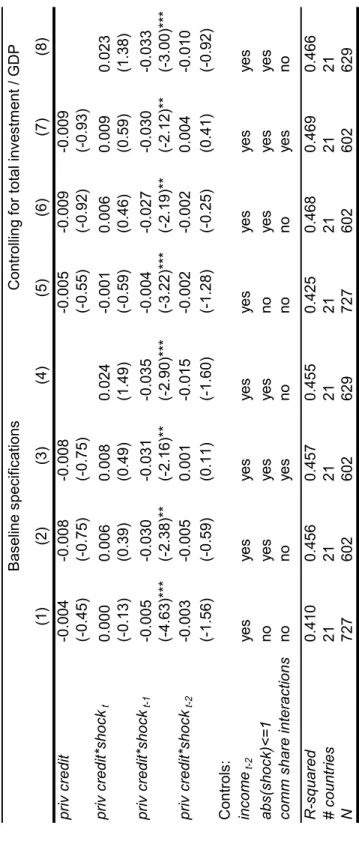
Using these empirical proxies, we find strong support for our model’s key predictions. First, the impact of shocks on the share of structural investment is greater in countries at lower levels of financial development. By contrast, no such effect is observed for the overall investment rate. Second, tighter credit amplifies the effects of shocks on output growth. Moreover, this result is not driven by the aggregate investment rate. Finally, financially underdeveloped countries feature less growth, more volatility, and a more strong negative correlation between growth and volatility.
Related literature. The growth and volatility effects of credit frictions have, of course, been
the subject of a voluminous literature, including Aghion, Banerjee and Piketty (1999), Aghion and Bolton (1997), Banerjee and Newman (1993), Bernanke and Gertler (1989), King and Levine (1993), and Kiyotaki and Moore (1997); see Levine (1997) for an excellent review and more references. We depart from this earlier work by studying how liquidity risk affects the cyclical composition of
2While R&D expenditure is another natural proxy for long-term productivity-enhancing investments, we opted
investment as opposed to the overall rate of investment. Many other papers—including Acemoglu and Zilibotti (1997), Aghion and Saint-Paul (1998), Barlevy (2004), Comin and Gertler (2004), Hall (1991), Gali and Hammour (1991), Koren and Tenreyro (2007), and Walde (2004)—do look at the allocation of investment across alternative uses; but they do not consider the impact of credit frictions and liquidity risk as our paper. Finally, Chevalier and Scharfstein (1996) propose a theory of countercyclical markups whose mechanics resemble those of our theory, once appropriately re-interpreted.3
Layout. The rest of the paper is organized as follows. Section 2 reviews some empirical and
theoretical considerations that motivate our exercise. Section 3 introduces the model. Section 4 analyzes the equilibrium composition of investment, while Section 5 derives the implications for growth and volatility. Section 6 contains the empirical analysis. Section 7 concludes.
2
Some motivating background
In an influential paper, Ramey and Ramey (1995) document a negative correlation between the volatility and the mean rate of output growth in a cross-section of countries. They show that this correlation survives a variety of controls and go on to argue that it admits a causal interpretation.4 Our paper is about thejoint determination of volatility and growth, rather than thecausal effect of the former on the latter. Nevertheless, the findings in Ramey and Ramey (1995) provide a certain motivation and guidance for our own theoretical and empirical explorations.
An negative effect of volatility on growth is consistent with the one-sector neoclassical growth model if risk discourages demand for investment more than it encourages the precautionary supply of savings, which is typically the case if the elasticity of intertemporal substitution is sufficiently high (Obstfeld, 1994; King and Rebelo, 1993; Jones, Manuelli and Stacchetti, 2000). A similar result can be obtained within the neoclassical growth model for the case of idiosyncratic investment risk (Angeletos, 2007). Such an effect is also consistent with models featuring financial frictions in the tradition of Bernanke and Gertler (1989): higher volatility may increase the likelihood of binding credit constraints and thereby reduce investment.
However, none of these stories seems to explain the observed negative correlation between volatility and growth. If these stories were the key behind this correlation, one would expect that controlling for the aggregate rate of investment would remove most of this correlation. As shown in columns 1-4 of Table 1, that’s not the case. In these columns, we re-estimate some of the basic
3
That paper argues that young firms have an incentive to keep their markups low in the hope of building up higher market shares, but this effect is likely to lower when bankruptcy risk is higher. The similarity to our paper then rests on re-interpreting the choice of a low markup as a long-term investment and the bankruptcy risk as liquidity risk.
4Complementary evidence is provided by Blattman, Hwang and Williamson (2004), Koren and Tenreyro (2007),
and others. See, however, Chatterjee and Shukayev (2005) and Ramey and Ramey (2006) for a debate on how sensitive these findings are to the particular measurement of output growth.
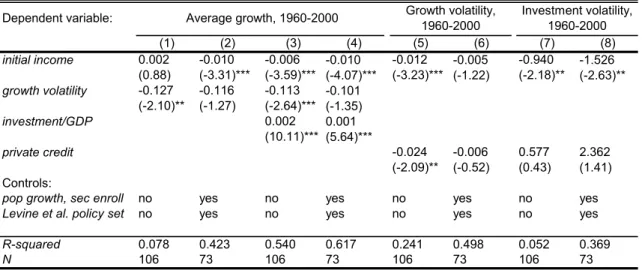
Table 1. Average growth, growth volatility and investment volatility
Dependent variable: Average growth, 1960-2000 Growth volatility, 1960-2000 Investment volatility, 1960-2000
(1) (2) (3) (4) (5) (6) (7) (8) initial income 0.002 -0.010 -0.006 -0.010 -0.012 -0.005 -0.940 -1.526 (0.88) (-3.31)*** (-3.59)*** (-4.07)*** (-3.23)*** (-1.22) (-2.18)** (-2.63)** growth volatility -0.127 -0.116 -0.113 -0.101 (-2.10)** (-1.27) (-2.64)*** (-1.35) investment/GDP 0.002 0.001 (10.11)*** (5.64)*** private credit -0.024 -0.006 0.577 2.362 (-2.09)** (-0.52) (0.43) (1.41) Controls:
pop growth, sec enroll no yes no yes no yes no yes
Levine et al. policy set no yes no yes no yes no yes
R-squared 0.078 0.423 0.540 0.617 0.241 0.498 0.052 0.369
N 106 73 106 73 106 73 106 73
Note: All regressors are averages over the 1960-2000 period, except for initial income and secondary school enrollment, which are taken for 1960. Growth and investment volatility are constructed as the standard deviation of annual growth and the share of total investment in GDP in the 1960-2000 period respectively. The Levine et al. policy set of controls includes government size as a share of GDP, inflation, black market premium, and trade openness. Constant term not shown. t-statistics in parenthesis. ***,**,* significant at 1%, 5%, and 10%.
specifications from Ramey and Ramey (1995) in our dataset. The point estimate of the volatility coefficient falls only by one tenth when the investment rate is included as an additional control. The data therefore suggest that the observed negative relation between volatility and growth isnot
channeled through the overall rate of saving and investment.
Morevoer, whereas there is suggestive evidence that credit access predicts both the mean and the volatility of the growth rate,5 a first pass at the data gives no indication that credit predicts the volatility of the aggregate investment rate. In our sample, the cross-country correlation between a country’s ratio of private credit to GDP—the measure of financial development usually used in the literature—and the country’s mean growth rate is 0.49, and the correlation between private credit and the variance of the growth rate is −0.42. By contrast, the correlation between private credit and the standard deviation of the ratio of investment to GDP is about zero (only −0.06). Moreover, when in columns 7 and 8 of Table 1 we repeat the same regressions as in columns 5 and 6 now using the standard deviation of the investment rate as the dependent variable, we find no relationship between the latter and the quality of the financial sector. Once again, this suggests that the volatility effects of credit constrains are not channeled through the overall rate of investment. Taken together, these observations indicate that one should look beyond the standard trans-mission channel—the response of aggregate saving and investment—in order to understand the interaction of effect of uncertainty and credit constraints on growth and volatility. Our approach
5If we include credit in the regressions of columns 1-4, then its effect on mean growth is positive, as standard in
then rests on shifting focus from the average rate of investment to its composition.
3
The model
We consider a closed economy that is populated by overlapping generations of a single type of agents, whom we call “entrepreneurs”. Each generation consists of a unit mass of entrepreneurs. Each entrepreneur lives for three periods and is endowed with one unit of labor in each period of her life. There is a single consumption good and two types of capital goods.
Consider an entrepreneur born in periodt. Her labor endowment, measured in efficiency units, is denoted byHt. We can think ofHtas the stock of human capital, skills, and other know-how that an entrepreneur has acquired by the time she starts engaging in productive activities. To simplify the analysis, we assume that this stock is fixed over the productive life of an entrepreneur and exogenous to her production choices. At the same time, we allow the growth rate ofHt to depend on the general equilibrium of the economy through a certain type of intergenerational spillover effects, similar in spirit to those in Lucas (1988); we specify these spillover effects later on. Finally, the preferences of this entrepreneur are given by
Ut=Ct,t+βCt,t+1+β2Ct,t+2 (1)
where Ct,t+n≥0 denotes her consumption during period t+n, for n∈ {0,1,2}, and β >0 is her discount factor.
In the first period of her life (period t), the entrepreneur has access to two CRS technologies that permit her to transform her effective labor to either of the two types of capital goods. In the subsequent two periods of her life, the entrepreneur has no more access to this capital-producing technology, but she can now use her stock of capital goods along with her endowment of labor to produce a consumption good under some other CRS technology. In particular, both types of investment have to be installed during the first period of the entrepreneur’s life (period t) and cannot be reallocated afterwards, but the one type becomes productive in the second period of her life (period t+ 1), while the other type becomes productive in the third period of her life (period
t+ 2). In what follows, we interpret the former type of capital as short-term investment and the latter one as long-term investment.
Consider first the production of capital goods. Since labor is the only input used in the produc-tion of the capital goods, the CRS assumpproduc-tion means that the corresponding producproduc-tion funcproduc-tions are linear. Let the technology of producing the short-term capital goods be Kt= θk,tHk,t, where
Hk,t is the amount of effective labor allocated to this technology, θk,t is the corresponding produc-tivity, and Kt is the produced amount of short-term capital goods. Similarly, let the technology of producing the long-term capital goods be Zt = θz,tHz,t, where Hz,t is the amount of effective labor allocated to this technology, θz,t is the corresponding productivity, and Kt is the produced
amount of short-term capital goods. We abstract from shocks to these productivities and, without any further loss of generality, we setθk,t=θz,t=θ for some fixedθ >0.6
Consider, next, the production of the consumption good. As mentioned already, short-term investment produces the consumption good with only a one-period lag. Thus, an entrepreneur who is born in periodt produces the following amount of the consumption good in periodt+ 1:
Yt,t+1 =At+1F(Kt, Ht) (2)
where At+1 is an exogenous aggregate productivity shock, Kt is the stock of short-term capital goods that the entrepreneur installed in period t,Ht is her effective labor, and F is a neoclassical production function. For simplicity, we assume thatF is Cobb-Douglas: F(K, H) =KαH1−α, for someα∈(0,1).
Long-term investment, on the other hand, takes one additional period in order to produce the consumption good. During this extra time, the entrepreneur may face an idiosyncratic “liquditiy” risk. By this we mean the following. In period t+ 1, the entrepreneur is hit by an idiosyncratic shock, denoted byLt+1 ≥0. This shock identifies a random expense, in terms of the consumption good, that the entrepreneur must incur in order to guarantee that her long-term investment remains intact. In particular, if the entrepreneur succeeds in covering this random expense, then she is able to produce the following amount of the consumption good in periodt+ 2:
Yt,t+2 =At+2F(Zt, Ht), (3)
whereAt+2 is the aggregate productivity shock in periodt+ 2, Ztis the stock of long-term capital goods that the entrepreneur installed in period t, and Ht is her effective labor. If, instead, the entrepreneur fails to cover this expense, then her long-term capital goods become obsolete and therefore her output in period t+ 2 is zero. We henceforth call this situation the “failure” or “liquidation” of the entrepreneur’s long-term investment.7
We further assume that, if the entrepreneur covers the liquidity shock in periodt+1, she recovers fully the associated expense in periodt+ 2 along with any foregone interest: conditional on paying
Lt+1 in period t+ 1, she receives β−1Lt+1 in period t+ 2. This assumption guarantees that this shock does not affect the net present value of the long-term investment of the entrepreneur; it only affects the intertemporal pattern of its gross costs and benefits.8 This assumption thus permits us
6In equilibrium, all entrepreneurs will choose the same levels of short-term and long-term investment (because they
have identical preferences, they face the same technologies and distribution of shocks, and their investment problem is strictly convex). For this reason, and to simplify the notation, we do not index individual investment choices by the identity of the entrepreneur, and instead useKt andZtto denote either individual or aggregate investment choices. However, one has to keep in mind that each entrepreneur is subject to an idiosyncratic liquidity risk, which implies that different entrepreneurs may end up with different realized incomes even though they make identical choices.
7
The fact that we model “failure” or “liquidation” as full, rather than partial, depreciation is only for simplicity.
8
to identify the shock Lt+1 as a pure liquidity shock: the presence of this shock has no effect on equilibrium allocations when markets are complete, but starts playing a crucial role once markets are incomplete. That being said, our key results do not hinge on this assumption. What is essential for our purposes is only that this shock induces a countercyclical liquidity risk when markets are incomplete; whether it may also happen to affect the present value of investment is of secondary importance, which is why we find it best to abstract from this effect.
In particular, we specify the financial structure of the economy as follows. First, we assume that the entrepreneurs can trade only a riskless short-term bond. Second, we impose an ad-hoc borrowing constraint that requires that the net borrowing of an entrepreneur in the first or second period of her life does not exceed a multiple µ of her contemporaneous income (where µ≥0). It follows that we can write the budget and borrowing constraints of the entrepreneur in these periods as follows: for the first period,
Ct,t+qt(Kt+Zt) =qtθHt+Bt,t and Bt,t≤µqtHt, (4) whereCt,tis her first-period consumption,qtis the unit price of capital goods at datet, qt(Kt+Zt) is her purchases of capital goods, Bt,t is her first-period borrowing (or saving, if this number is negative), and qtθHt is her income from the production and sale of capital goods, while for the second period,
Ct,t+1+Lt+1et,t+1=Yt,t+1+Bt,t+1−(1 +Rt)Bt,t and Bt,t+1 ≤µYt,t+1, (5)
where Ct,t+1 is her second-period consumption, Lt+1 is the liquidity shock, et,t+1 is an indicator function that takes the value 1 if the entrepreneur covers this shock and 0 otherwise, Bt,t+1 is her second-period borrowing, Yt,t+1 is her income from short-term investment, and Rt is the risk-free rate between periodstandt+ 1. In the third period, on the other hand, we impose that no further borrowing is allowed because the entrepreneur will die after this period. Her budget constraint is thus given by
Ct,t+2= (Yt,t+2+β−1Lt+1)et+1+ (1 +Rt+2)Bt,t+1, (6) where Ct,t+2 is her third-period consumption,Yt,t+2 is her income from long-term investment and
β−1Lt+1 is the recovery of the previous-period liquidity expense.
To close the model, we need to specify the dynamics of the stock of human capital (Ht), the stochastic process of the aggregate productivity shock (At) and the idiosyncratic liquidity shock (Lt). We do so as follows.
For the stock of human capital (or level of know-how), we assume the following law of motion:
Ht+1= Γ(Ht,Z˜t, Kt)
where ˜Zt denotes the amount of long-term investment that survives the liquidity shock (to be de-termined in equilibrium) and where the function Γ is continuous and increasing in all its arguments.
To guarantee a balanced-growth path, we assume that Γ is homogenous of degree 1. We further assume that, for anyH and any given sumZ+K, Γ(H, Z, K) increases with the ratioZ/K. With this assumption we seek to capture the idea that many long-term investments such as education, firm entry, R&D, and the like appear to be relatively more conducive to productivity growth than short-term investments in working capital, machines, and the like. This in turn will permit us to spell out the potential implications of our results for the dynamics of growth without going into the deeper micro-foundations of productivity growth.
Next, for the productivity shock, we assume that its logarithm follows an AR(1) process:
logAt=ρlogAt−1+ logνt (7)
where νt is the innovation in the productivity shock—a random variable that is i.i.d. over time, with mean normalized to E[νt] = 1, positive higher moments, and compact support [νmin, νmax], with 0< νmin< νmax <∞—and whereρ∈(0,1) parameterizes the persistence of the productivity shock. The key property we seek to capture with this specification is that the business cycle features both some persistence (ρ >0) and some mean-reversion (ρ <1). This is essential for our argument. The log-linearity, instead, is not essential; it only buys us some tractability in computing conditional expectations for future productivity shocks.
Finally, for the liquidity shock, we assume that it grows in proportion to Ht so as to guarantee that the economy admits a balanced growth path along which the impact of the liquidity risk does not vanish as the economy grows. Formally, we let `t+1 ≡Lt+1/Ht denote the “normalized” level of the liquidity shock and impose that the distribution of `t+1 is invariant over time; we then let [0, `max] be the support of this distribution and Φ its c.d.f..9 We further impose that
`max> AmaxF(θ,1),where`maxandAmax≡νmax/(1−ρ) are, respectively, the maximum possible realizations of the liquidity shock and of the productivity shock; as it will become clear, this restriction guarantees that the entrepreneur will fail to meet the maximal liquidity shock when credit markets are sufficiently tight (µ is sufficiently small). Finally, to maintain tractability, we impose a power-form specification: Φ(`) = (`/`max)φ when` < `max, for some φ >0, and Φ(`) = 1 when `≥`max.10
9An alternative specification of the liquidity shock that would also guarantee the existence of such a
balanced-growth path is one that specifies the shockLt+1 as proportional to the levelZt+1 of the enterpreneur’s long-term
investment. In this case, the exogenous, stationary shock would be given by `t+1 ≡ Lt+1/Zt+1. Furthermore,
thanks to the CRS property of the production function, one could then interpret the probability thatLt+1 ≤Xt+1
interchangeably either as the probability that the entire long-term investment of the entrepreneur survives to period
t+ 2, or as thefraction of her long-term capital stock that survives to periodt+ 2. Finally, because this specification retains the key property of our model, namely that the liquidity risk is countercyclical, it also does not affect the core of our key predictions. However, this specification is more cumbersome analytically, which is why we opted for the simpler one we have assumed.
10
Remarks. There are various interpretations of what the two types of investment and the liq-uidity shock may represent. The short-term investment might be putting money into one’s current business, while the long-term productivity-enhancing investment may be starting a new business. Or, the short-term investment may be maintaining existing equipment or buying a machine of the same vintage as the ones already installed, while the long-term investment is building an additional plant, building a research lab, learning a new skill, or adopting a new technology. Similarly, the liquidity shock might be an extra cost necessary for a newly-adopted technology to be adapted to evolving market conditions; or a health problem that the entrepreneur needs to deal with; or some other idiosyncratic shock that can ruin the entrepreneur’s business unless she can repair the dam-age from it. Finally, the fact that long-term productivity-enhancing investments such as starting up a new business, learning a new skill, adopting a new technology, or undertaking a new R&D project are largely intangible and non-verifiable may justify our implicit assumption that a large portion of these investments is not collateralizable—and hence that these investments may get dis-rupted by liquidity shocks even if they have positive net present value. In this regard, although we abstract from the micro-foundations of liquidity constraints, we are essentially building on the insights of the related literature on moral hazard and credit constraints, such as Holmstrom and Tirole (1998) and Aghion, Banarjee and Piketty (1999). Indeed, note that the latter paper provides a microfoundation of the particular borrowing constraint we assume in this paper.
4
Equilibrium composition of investment
In this section we analyze the equilibrium composition of investment, starting first with the case where markets are perfect and then moving to the case where credit constraints are binding. Our model is designed so that the characterization of the equilibrium composition of investment can be derived without characterizing the equilibrium dynamics of Ht. This highlights that the core contribution of our paper regards the cyclical composition of investment. We will spell out the implications of our results for output volatility and growth in a subsequent section.
4.1 Complete markets
Suppose that credit markets are perfect and consider an entrepreneur born in periodt. Because the entrepreneur can borrow as much as she wishes in the second period of her life, she can always meet her liquidity shock, should she find it desirable to do so. Because of the linearity of preferences, the equilibrium interest rate is pinned down by Rt=β−1. It follows that the net present value of meeting the liquidity shock is (Yt,t+2+β−1Lt+1)−Rt+1Lt+1 =Yt,t+2 =At+2F(Zt, Ht)≥0, which guarantees that it is always optimal for the entrepreneur to meet her liquidity shock.
liquidity risk faced by the entrepreneur. When the elasticity of Φ is not constant, our equilibrium characterization can be interpreted as a log-linear approximation around the steady state.
Next, the budget constraints along with the fact that Rt=β−1 imply that the present value of the entrepreneur’s consumption—also her lifetime utility—is pinned down by the following:
Ut = Ct,t+βCt,t+1+β2Ct,t+2
= qt(θHt−Kt−Zt) +β(Yt,t+1−Lt+1) +β2(Yt,t+2+β−1Lt+1) = qt(θHt−Kt−Zt) +βAt+1F(Kt, Ht) +β2At+2F(Zt, Ht)
We infer that the optimal investment problem of the entrepreneur can be reduced to the following: max
Kt,ZtEt
βAt+1F(Kt, Ht) +β2At+2F(Zt, Ht)−qtKt−qtZt
Let kt≡Kt/Ht and zt≡Zt/Ht denote the “normalized” levels of short- and long-term invest-ment. We can then restate the entrepreneur’s problem as follows:
max kt,zt Et
βAt+1f(kt) +β2At+2f(zt)−qtkt−qtzt
Because f is strictly concave, the solution to the above problem, for given qt, is uniquely pinned down by the following first-order conditions:
βEt[At+1f0(kt)] =qt and β2Et[At+2f0(zt)] =qt. (8) That is, the entrepreneur equates the marginal cost of the two types of investment (the price qt) with their expected marginal profit.
The individual entrepreneur takes the price of capital goods,qt, as exogenous to her choices. In equilibrium, however, this price adjusts to make sure that the aggregate excess demand for capital goods is zero. In other words, the equilibrium investment levels must satisfy the resource constraint
Kt+Zt=θHt, where, recall, θ is the productivity of new-born entrepreneurs in the production of capital goods. Equivalently, the normalized levels must satisfy
kt+zt=θ.
Combining this with (8), we infer that the equilibrium composition of investment is pinned down by the following condition:
Et[At+1f0(θ−zt)] =βEt[At+2f0(zt)] (9) This condition has a straightforward interpretation: it equates the marginal value of long-term investment (on the right-hand side) with its opportunity cost (on the left-hand side).
To complete the characterization of the equilibrium, we only need to ensure that there are enough aggregate resources to pay for the liquidity shocks in each period. To do so, we henceforth impose that the parameters of the economy satisfy lmean < Aminf(θ−zmax), where zmax is the solution to condition (8) whenAt=Amin,and whereAminandlmeanare, respectively, the minimum productivity level and the mean liquidity shock.11 We then reach our first main result.
11
Proposition 1 Suppose that credit markets are perfect. (i) The equilibrium exists and is unique.
(ii) There exists a continuous function z∗ : R+ → (0, θ) such that the equilibrium levels of
short-term and long-term investment are given, respectively, by kt=θ−z∗(At) and zt=z∗(At).
(iii) The function z∗ is strictly decreasing. That is, the share of long-term investment decreases with a positive innovation in productivity.
Proof. By the AR(1) specification of the process for the productivity shock, we have that
Et[At+1] = Et[νt+1Aρt] = A ρ
t and Et[At+2] = Et[Et+1[At+2]] = Et[Aρt+1] = Et[(vt+1Aρt)ρ] = χA ρ2
t , where χ≡E[νtρ]>0. Rearranging condition (9), and using the aforementioned facts, we get that the equilibriumztis pinned down by the following equation:
f0(zt) f0(θ−z t) = Et[At+1] βEt[At+2] = A ρ(1−ρ) t βχ
Note that the left-hand side of the above equation is continuous and decreasing in zt, while the right-hand side is continuous and increasing in At. Furthermore, the left-hand side tends to +∞
(respectively, 0) as zt → 0 (respectively, θ). Parts (ii) and (iii) then follow from the Implicit Function Theorem. Finally, part (i) follows from part (ii) along with the fact that the assumption
lmean < Aminf(θ−zmax),where zmax =z∗(Amin), guarantees that consumption is positive in all states. QED
The logic behind this result is very basic and hence likely to extend to richer environments. As long as there is mean-reversion in the business cycle, profits anticipated in the near future are likely to be more pro-cyclical than profits anticipated in the distant future. Moreover, the return to short-term investment depends more heavily on profits in the near future, while the return to long-term investment depends more heavily on profits in the distant future. It follows that the return of short-term investment is likely to be more procyclical than the return to long-term investment and, therefore, the composition of investment is likely to shift towards a relatively higher share of long-term investment during recessions than during booms.
At the core of this result is a particular type of opportunity-cost effect: the opportunity cost of long-term investment, in terms of forgone short-term investment opportunities, is higher in booms than in recessions. This opportunity-cost effect, which induces countercylicality in the share of long-term investment, is present independently of whether credit markets are perfect or not; but once markets are imperfect, an additional, countervailing effect emerges. We move on to identify this additional effect in the next section.
Remark. Proposition 1 stated the cyclical properties of the composition of investment in terms
of its co-movement with the productivity shock. However, it is straightforward to translate these properties in terms of the co-movement of the two types of investment with aggregate output (which
is the canonical definition of cyclical properties). To see this, note that the equilibrium level of GDP, evaluated in units of the consumption good, can be written as follows:
GDPt=Atf(kt−1) +Atf(zt−2) +qtkt+qtzt. (10)
The first two terms on the right-hand side capture the value added of the consumption sector, while the last two terms capture the value added of the investment sector. Clearly, the first two terms increase with a positive innovation in At. By Proposition 1 and the fact thatqt=E[At+2]f0(zt) in equilibrium, we have that qt also increases with a positive innovation in At. Since kt+zt = θ is constant, we conclude thatGDPt, too, increases with a positive innovation in At. It follows that the contemporaneous covariance between GDP and the share of long-term investment is indeed negative.
4.2 Incomplete markets
Consider now the case where credit markets are imperfect. Once again, the linearity of preferences guarantees that Rt = β−1. But now the entrepreneur is not completely indifferent about the timing of her consumption and the pattern of her borrowing and saving. In particular, because the probability of failing to meet the liquidity shock is positive, the entrepreneur finds it strictly optimal to consume zero in the first period of her life—for doing so maximizes the availability of funds in the second period and thereby minimizes the probability of failure. Furthermore, whenever the entrepreneur has enough funds herself in the second period to cover her liquidity shock, or can borrow enough funds to meet this goal, she will always find it optimal to do so. It follows that the entrepreneur covers her liquidity shock if and only if Lt+1≤Xt+1, where
Xt+1 ≡(1 +µ)Yt,t+1+Rtqt(θHt−Kt−Zt).
The latter measures the total liquidity available to the entrepreneur during periodt+ 1: it is given by the income of the entrepreneur in that period, plus the maximal borrowing that is available to her in that period, plus any savings from the (net) sale of capital goods in the previous period.
Combining the aforementioned observations with the budget constraints, we infer that the present value of the entrepreneur’s consumption—also her lifetime utility—is pinned down by the following:
Ct,t+βCt,t+1+β2Ct,t+2 = qt(Ht−Kt−Zt) +βAt+1F(Kt, Ht) +β2At+2F(Zt, Ht)et+1
whereet+1= 1 ifLt+1 ≤Xt+1 and et+1= 0 if Lt+1 > Xt+1.Letting xt+1 ≡Xt+1/Ht, we can thus state the entrepreneur’s problem as follows:
max kt,zt Et
βAt+1f(kt) +β2λt+1At+2f(zt)−qtkt−qtzt
whereλt+1 ≡Φ (xt+1) is the probability that the entrepreneur will have enough funds to cover the liquidity shock. Equivalently, 1−λt+1 measures the “liquidity risk” faced by the entrepreneur: it is the probability that long-term investment will become obsolete due to the unavailability of enough liquidity in periodt+ 1.
The first-order condition of the entrepreneur’s problem with respect to kt gives
βEt[At+1f0(kt)] +β2Et[∂λt∂kt+1At+2f(zt)] =qt,
while the one with respect tozt gives
β2Et[λt+1At+2f0(zt)] +β2Et[∂λt∂zt+1At+2f(zt)] =qt.
Combining these two first-order conditions gives the following arbitrage condition between the two types of investment: Et[At+1f0(kt)] =βEt[(1−τt+1)At+2f0(zt)], (11) where τt+1 ≡(1−λt+1) + ∂λt+1 ∂kt − ∂λt+1 ∂zt f(zt) f0(zt) (12)
The quantity τt+1, which is isomorphic to a tax on the return of long-term investment, identifies the wedge that credit frictions introduce between the two types of investment. Understanding the cyclical properties of this wedge is the key to understanding how credit frictions impact the cyclical composition of investment. In what follows we thus seek to gain further insight in the equilibrium determination of this wedge.
We start by observing that the wedge τt+1 comprises two terms. The first term captures the probability of failure; the second term captures the marginal change in this probability caused by a reallocation of investment from the long-term opportunity to the short-term one. The first term would emerge even if the probability of failure were exogenous to the choices of the entrepreneur; the second term, instead, highlights the endogeneity of the liquidity risk. Whenxt+1> `max (that is, when the entrepreneur has enough liquidity to meet even the highest possible liquidity shock), both terms are zero and the wedge vanishes. When, instead,xt+1 < `max, the probability of failure is positive. Furthermore,12 ∂λt+1 ∂kt − ∂λt+1 ∂zt = Φ 0(x t+1)(1 +µ)At+1f0(kt)/`max>0, (13) which means that shifting a unit of capital from the long-term to the short-term investment op-portunity necessarily reduces the probability of failure; this is simply because such a shift increases the available liquidity in periodt+ 1. It follows thatτt+1 is strictly positive wheneverxt+1< `max.
12
Note thatxt+1= (1 +µ)At+1f(kt) +Rtqt(θ−kt−zt), implying that∂λ∂kt+1
t = Φ 0 (xt+1)[(1 +µ)At+1f0(kt)−Rtqt] and ∂λt+1 ∂zt = Φ 0
We henceforth restrict attention to situations where credit constraints are sufficiently tight that the liquidity risk and the associated wedge are bounded away from zero. That is, we assume that the equilibrium satisfies xt+1 < `max, so that λt+1 <1 and τt+1 >0. Note then that, while this is an assumption on equilibrium objects, it is easy to find a restriction on the exogenous parameters of the economy that guarantees that this assumption holds. In particular, this is the case if we let
µ <µ¯, where ¯µ >0 solves (1 + ¯µ)Amaxf(θ) =`max.
Finally, we consider the cyclical properties of this wedge. Using xt+1 = (1 +µ)At+1f(kt) into condition (13), we get that ∂λt+1
∂kt −
∂λt+1
∂zt =φλt+1 f0(kt)
f(kt). Substitution this into (12), we infer that condition (11) can be restated as follows:
Et At+1f0(θ−zt) 1 +βφλt+1 At+2f(zt) At+1f(kt) =βEt λt+1At+2f0(zt) (14) To gain further insight, let us momentarily ignore the underlying uncertainty about aggregate productivity. We can then drop the expectation operators from both conditions (11) and (14). Since the two conditions are equivalent, we infer that the wedge is also given by
τt+1 = 1−
λt+1
1 +βφλt+1AtAt+2+1ff((ztkt))
,
which is decreasing in λt+1 and increasing in the ratio AtAt+1+2ff((ktzt)). Intuitively, one would expect the probability of survivalλt+1 to be higher in a boom, because of the improved availability of liquidity. One would also expect the ratio At+2f(zt)
At+1f(kt) to be lower in a boom, because of the mean-reversion in
the business cycle. One would thus expect the wedgeτt+1to be lower in a boom than in a recession. Other things equal, this countercyclicality of the wedgeτtwould tend to boost long-term invest-ment during a boom. However, the opportunity-cost effect that we encountered under complete markets is still present and contributes in the opposite direction. Therefore, one would expect the share of long-term investment to be procyclical if and only if the countercyclicality of the wedgeτt+1 is sufficiently strong to offset the countervailing opportunity-cost effect. We verify these intuitions in the following proposition, which is our second main result.
Proposition 2 Suppose that credit constraints are sufficiently tight that the liquidity risk is
non-zero in all states of nature, which is necessarily the case if µ <µ¯. (i) The equilibrium exists and is unique.
(ii) There exists a continuous function z such that the equilibrium composition of investment is given by kt=θ−z(At, µ) and zt=z(At, µ).
(iii) This function satisfies z(A, µ) < z∗(A) for all (A, µ), and is decreasing in µ. That is, credit constraints depress the share of long-term investment below its complete-market value, and the more so the tighter they are.
(iv) Suppose further that φ >1−ρ. Then the function z(A, µ) is increasing in A. That is, the share of long-term investment increases with a positive innovation in productivity.
Proof. By the assumption that µ <µ¯or, more generally, that the liquidity risk is non-zero, we have that xt+1 < `max and λt+1 = (xt+1/`max)φ, where xt+1 = (1 +µ)At+1f(kt) and kt =θ−zt. Using these facts, we can restate (14) as follows:
Et h At+1f0(kt) 1 +βφ`−maxφ (1 +µ)φAφt+1−1f(kt)φ−1At+2f(zt) i =βEt h `−maxφ (1 +µ)φAφt+1f(kt)φAt+2f0(zt) i
Next, using the log-linear AR(1) specification of the productivity shock to compute the various expectations involved in the above condition, we can rewrite this condition as follows:
Aρtf0(kt) 1 +βφδ(1 +µ)φAtρ(φ−1)f(kt)φ−1Aρ 2 t f(zt) =βδ(1 +µ)φAtρφf(kt)φAρ 2 t f 0(z t), whereδ is a positive constant defined byδ≡`max−φ E[νtρ+φ]. Finally, rearranging the above gives the following: f0(zt) f0(θ−z t) = A ρ(1−ρ−φ) t βδ(1 +µ)φf(θ−z t)φ +φ f(zt) f(θ−zt) (15) Note that the left-hand side is continuous and decreasing inzt,while the right-hand side is contin-uous and increasing in zt. Furthermore, the right-hand side is continuous and decreasing in µ; it is continuous inAt; and it is increasing inAt [resp., decreasing] if and only if 1−ρ−φ >0 [resp., 1−ρ−φ <0]. Parts (ii), (iii) and (iv) then follow from the Implicit Function Theorem. Finally, part (iii) implies that, for all (A, µ), z(A, µ) < zmax ≡ z∗(Amin). Along with the assumption
lmean< Aminf(θ−zmax), this guarantees that consumption is positive in all states. Part (i) then follows from this fact together with part (ii). QED
The property that the share of long-term investment is lower than under complete markets is a direct implication of our result that τt+1 > 0, namely that the liquidity shock introduces a positive wedge between the marginal products of the long-term and the short-term investment. As mentioned already, this wedge reflects, not only the positive probability that the long-term invest-ment will get disrupted by a sufficiently high liquidity shock, but also the consequent precautionary motive for short-term investment.
Part (iii) of the above proposition then extends this result by showing that the share of long-term investment decreases mononotinically with the tightness of the borrowing constraints. Intuitively, as credit constraints become tighter, the probability of disruption increases and the precautionary motive gets reinforced, implying that long-term investment is further depressed.
Turning to the cyclical behavior of the composition of investment, we first note that this is governed by two conflicting effects. On the one hand, a positive productivity shock raises the opportunity cost of long-term investment (the marginal product of short-term investment). This
opportunity-cost effect, which is equally present under complete and incomplete markets, pushes the economy to shift resources away from long-term investment during a boom. On the other hand, a positive productivity shock also improves the availability of liquidity, thereby reducing the
probability of disruption, the precautionary motive for short-term investment, and the wedgeτt+1. Thisliquidity-risk effect, which emerges only when markets are incomplete, pushes the economy in the opposite direction: it motivates entrepreneurs to invest relatively more in long-term projects during a boom.
Part (iv) of the above proposition establishes that the liquidity-risk effect dominates if and only if φ is sufficiently high relative to 1−ρ. Intuitively, this is because a higher φ strengthens the liquidity-risk effect by raising the cyclical elasticity of the liquidity risk, while a higher ρ dampens the opportunity-cost effect by increasing the persistence of the business cycle.13
Comparing the result of Proposition 2 with that of Proposition 1, we conclude that the share of long-term investment turns from countercyclical under complete markets to procyclical when two conditions are satisfied: credit constraints are tight enough that they are always binding (µ <µˆ); and the implied liquidity risk is sufficiently procyclical (φ > 1−ρ). This result thus provides us with a very sharp contrast between complete and incomplete markets—a sharp contrast that best illustrates the theoretical contribution of our paper. In what follows, we discuss how our results need to be qualified if one of the above two conditions fails– the sharpness is then somewhat lost, but the essence remains intact.
4.3 Discussion
When the conditions µ <µ¯ and φ >1−ρ are violated, the sharp contrast between complete and incomplete markets that we obtained in the preceding analysis is lost. In particular, whenµis high enough, the borrowing constraint stops binding for sufficiently high productivity shocks, and the liquidity risk vanishes for these states. The share of long-term investment is then locally decreasing with the productivity shock, at least for an upper range of the state space. When, on the other hand, φis less than 1−ρ, the share of long-term investment is countercyclical no matter whether the credit constraint is binding or not.
Nevertheless, a weaker version of our result survives. As long as µ is low enough that the probability of disruption is positive for a non-empty subset of the state space, the liquidity-risk effect that we discussed earlier remains present for this same subset of the state space: it might vanish for sufficiently high states, and it might never be strong enough to offset the conflicting opportunity-cost effect, but it always contributes some procyclicality in the share of long-term investment relative to the complete-markets case. In this sense, credit frictions may not always turn the countercycality of long-term investment upside down, but they do tend to mitigate it.
Finally, note that as long as the liquidity risk is bounded away from zero (which is necessarily the case whenµ < µ¯), the cyclical elasticity of the liquidity risk is pinned down by φalone, while
13
This intuition suggest thatρshould not be interpreted too literally as the autocorrelation of the exogenous shock, but rather more generally as the persistence of the impulse response of output to the underlying shock.
µ matters only for the level of the liquidity risk. This explains why the cyclical properties of the composition of investment in the above proposition are governed solely by a comparison ofφwith
ρ and not by µ. However, when the liquidity risk vanishes in some states (which is the case for
µ sufficiently high), then µ starts mattering also for the cyclical elasticity of the liquidity risk. In particular, a lower µ implies a smaller range of At for which the liquidity risk vanishes, and therefore a larger subset of the state space for which the procyclical liquidity-risk effect is present. Combining these observations, we conclude that the core theoretical prediction of our paper can be stated as follows.
Main Prediction. Other things equal, tighter credit constraints make it more likely that the share
of long-term investment increases with a positive productivity shock.
We expect this prediction to extend well beyond the specific model of this paper, for it rests only on two highly plausible properties: that long-term investment is relatively more sensitive to liquidity risk, by the mere fact that it takes longer to complete; and that liquidity risk is more severe in recessions than in booms. We will test this prediction in Section 6 below.
5
Reinterpretation and additional results
In this section we provide a re-interpretation of the productivity shock that illustrates that our insights need not be unduly sensitive to the details of the underlying business-cycle shocks, while also facilitating our subsequent empirical investigation. We then proceed to study the predictions that our theory makes regarding the dynamics of output growth.
5.1 Reinterpreting the productivity shock
In our model, the source of the business cycle is a TFP shock. However, one should not take this too literally. Rather, the productivity shock in our model is meant to capture more broadly a variety of supply and demand shocks that may cause variation in firm profits and thereby in the returns of the two types of investment. For example, in our empirical analysis, we seek to re-interpret the productivity shock as a particular type of terms-of-trade shock, because we find this to be best from the perspective of econometric identification. We now present a variant of our model that justifies this re-interpretation.
The economy is now open to international trade. In particular, the economy continues to produce a single consumption good, but can now export this good to the rest of the world and can import from it a variety of other consumption goods. In addition, the economy imports a particular intemediate input—think of it as oil—that is used in the production of the domestic good.
Consider an entrepreneur born in period t. Re-interpretCt,t+n as a CES composite of all the goods the entrepreneur consumes and let Pc,t denote the price index of this composite relative to
the domestic good. Next, let Pm,t denote the price of the aforementioned imported intermediate input relative to the domestic good; letMtdenote the quantity of this input that the entrepreneur purchases; and let the technologies the entrepreneur uses to produce the domestic good in periods
t+ 1 andt+ 2 be given, respectively, by
Yt,t+1 = (Mt+1)1−η(At+1F(Kt, Ht))η and Yt,t+2 = (Mt+2)1−η(At+2F(Zt, Ht))η
Finally, let ˜Yt,t+n denote the real value (in terms of the consumption composite) of the net income that the entrepreneur enjoys in period t+nonce she has optimized over the use of the imported input: ˜ Yt,t+n≡ 1 Pc,t+1 max Mt+n [Yt,t+n−Pm,t+nMt,t+n].
It is straightforward to characterize the optimal use of the intermediate input and thereby to show that ˜ Yt,t+1= ˜At+1F(Kt, Ht) and Y˜t,t+1= ˜At+2F(Zt, Ht), where ˜ At≡ηPc,t−1P −1−ηη m,t At
is a composite of the productivity shock and the relative prices of the imported goods. We can then repeat the entire analysis of our baseline model simply by replacingYt,t+nwith ˜Yt,t+n, andAt with ˜At. Therefore, we can indeed reinterpret a positive productivity shock as a reduction in the relative price of either the imported consumption goods or the imported intermediate input—that is, as a positive shock to the country’s terms of trade.
Of course, this exact equivalence between productivity and terms-of-trade shock may not hold in richer models.14 Rather, the purpose of the above example is to clarify that we wish to take the productivity shock only as a metaphor for a variety of aggregate shocks that may affect firm profits and investment returns. The choice of our empirical proxy for these shocks will then be guided primarily by econometric considerations.
5.2 Propagation and amplification
We now study the predictions of our model for the endogenous component of productivity, as captured by the Ht. Recall that the law of motion for Ht is assumed to be Ht+1 = Γ(Ht,Z˜t, Kt), where Γ is homogeneous of degree 1 and where ˜Zt is the amount of long-term investments that survive the liquidity shock. Using this along with the facts that, in equilibrium, ˜Zt = λt+1Zt,
Zt=ztHt, and Kt= (θ−zt)Ht, we infer the equilibrium growth rate ofH is given by
Ht+1
Ht
=γ(zt, λt+1)
14For example, if there is both a tradeable and a non-tradeable sector, a terms-of-trade shock will increase returns
in the tradeable sector much like a productivity shock, but will also cause a reallocation across the two sectors that is unlike the symmetric effect of an aggregate productivity shock.
where the functionγ is defined by γ(z, λ) ≡Γ(1, λz, θ−z). Furthermore, by the assumption that Γ(H, Z, K) increases withZ for givenK and that it increases with the ratioZ/K for givenZ+K, we have that the functionγ is increasing in both its arguments. Using these observations along with our results regarding the cyclical composition of investment, we reach the following characterization of the growth rate of the efficiency of labor.
Proposition 3 (i) There exist functions h∗ and h such that Ht+1/Ht = h∗(At) when markets
are complete and Ht+1/Ht =h(At, νt+1, µ) when markets are incomplete (where νt+1 denotes the
innovation in productivity between periods tand t+ 1).
(ii) Suppose µ <µ¯, or more generally that the liquidity risk is bounded away from zero. Then,
h(At, νt+1, µ) is necessarily lower than h∗(At), it is increasing in µ, and it is increasing in νt+1.
That is, the endogenous component of productivity growth is lower under incomplete markets than under complete markets, and the more so the lower µor the lower the innovation in productivity.
(ii) Suppose further that φ > 1 −ρ. Then, h(At, νt+1, µ) is increasing in At. In contrast,
h∗(At) is necessarily decreasing in At. That is, the endogenous component of productivity growth
increases with the beginning-of-period productivity under incomplete markets, whereas it decreases with it under complete markets.
Proof. Part (i) follows from our preceding discussion, letting
h∗(A)≡γ(z∗(A),1) and h(A, ν, µ)≡γ(z(A, µ), λ(A, ν, µ))
where λ(A, ν, µ) ≡ Φ((1 +µ)Aρνf(θ−z(A, µ)) identifies the equilibrium probability of survival. Part (ii), on the other hand, follows from combining the monotonicity of γ with the properties that z(A, µ) < z∗(A) and λ(A, ν, µ) < 1 (from part (i) of Proposition 2) and the observation that λ(A, ν, µ) increases with ν. Finally consider part (iii). The claim that h∗(At) decreases with
At follows directly from the result that z∗(At) is decreasing in At (from Proposition 1) and the monotonicity of γ. Turning to the incomplete-markets growth rate, we know (from Proposition 2) thatzt=z(At, µ) increases with bothAt andµ. It is possible to show thatλt=λ(At, νt+1, µ) also increases with At and µ. Towards this goal, rewrite condition (15) as follows:
f0(zt) f0(θ−zt) −φ f(zt) f(θ−zt) = Aρt(1−ρ) βδλt+1νt−+1φ
Note then that the left-hand side is decreasing inzt, and thereby decreasing in Atand µ, while the right-hand side is increasing in At and independent of µ. It follows that λt+1 is indeed increasing in At and µ, as claimed. The monotonicity of γ then implies thath(At, νt+1, µ) is also increasing inAt and µ. QED
This result follows from the combination of our earlier results regarding the composition of investment with the property that long-term investments are relatively more conducive to produc-tivity growth than short-term ones. While we have only assumed the latter property, rather than
derive it from deeper micro-foundations, we nevertheless think that this assumption is both highly plausible and empirically relevant. Furthermore, note that this result would only be re-inforced if we let the rate of productivity growth depend on the fraction of long-term investments that survive, as opposed to its entire level; the property that some long-term investments get disrupted would then further depress the growth rate ofH, while the property that this fraction is countercyclical would further strengthen the procyclicality of the growth rate of H under incomplete markets. Finally, translating this result in terms of GDP growth, we reach the following two testable predictions:
Auxiliary predictions. (i) In the short run, tighter credit constraints amplify the response of
output to exogenous business-cycles shocks. (ii) In the long run, they lead to lower mean growth.
The second prediction is consistent with prior work studying the empirical cross-country rela-tionship between measures of financial development and the long-run growth rate. The first one, on the other hand, will be an important part of our own empirical investigation in Section 6.
5.3 On the relationship between volatility and growth
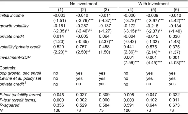
Combining these last two predictions, we infer that countries with tighter credit constraints should experienceboth lower and more volatile growth rates. Thus, as long as one fails to control for the tightness of credit constraints, our model predicts that one should find a negative partial cross-country correlation between growth and volatility.
This observation provides one possible interpretation of the empirical findings of Ramey and Ramey (1995) through the lens of our model: the negative cross-country correlation between growth and volatility observed in the data may reflect aspurious correlation induced by unmeasured cross-country differences in financial development, rather than any causal effect of uncertainty on growth. Moreover, this negative correlation need not diminish once one controls for the level of aggregate investment, for what matters is its composition.
Another possible interpretation of the aforementioned empirical relationship through the lens of our model rests on thecausaleffect of uncertainty on the composition of investment, and thereby on productivity growth. Unfortunately, we have been unable to provide any general result on this front because the comparative statics of the equilibrium with respect to the variance of the productivity shock are quite complex and involve various additional effects. However, the following discussion sheds some light on why it is quite plausible that more volatility may cause a lower mean growth rate within the context of our model.
As long as credit constraints are neither too tight nor too loose, we expect them to bind for sufficiently low productivity shocks but not for sufficiently high shocks. This makes it quite likely that the probability of survival,λt+1, is a concave function of the productivity shock—and therefore that the mean level of this probability decreases with a mean-preserving spread in the productivity
shock. In other words, we expect higher aggregate volatility to increase the mean level of the idiosyncratic liquidity risk. But then we also expect higher volatility to depress the growth rate of the economy, both by reducing the demand for long-term investments (an ex-ante effect) and by reducing the survival rate of such long-term investment (an ex-post effect).
Furthermore, as long as credit constraints are neither too tight nor too loose, we expect the share of long-term investment, zt, to be an increasing function of the productivity shock when the shock is sufficiently low (so that the borrowing constraint binds), and a decreasing function of it when the shock is sufficiently high (so that the borrowing constraint does not bind). In this sense, we expect the share of long-term investment to be a concave function of the productivity shock, much like the probability of survival. But then we also expect the mean level of long-term investment to fall when volatility is higher, once again contributing to lower growth.
The combination of these observations makes us believe that a negative causal effect of volatility on mean growth is quite likely within the context of our model. However, we need to qualify this prediction with the following important observation. If the credit constrains are sufficiently tight that the probability of survival is zero (or nearly zero) even for the mean productivity shock, then a mean preserving spread in the productivity shock may actually increase the mean probability of survival, and thereby stimulate long-term investment and growth. In essence, average conditions in the economy are then so dire that higher volatility stimulates the economy by increasing the likelihood of “resurrection”.
While this resurrection effect is theoretically possible, we do not expect it to be particularly relevant in practice: if the average situation were so dire, agents would probably have opted to avoid the liquidity risk altogether, perhaps by taking some other option that is not allowed in our model (such as abstaining completely from entrepreneurial activity and investment). We therefore expect that the most likely scenario is one where more volatility increases the average liquidity risk, thereby further distorting the composition of investment and depressing productivity growth.
6
Empirical analysis
In this section, we use data on a panel of 21 OECD countries to provide evidence in support of the key predictions of the model. We proxy for the long-term investment rate zt in the model with the share of structural investment in total private investment; the exogenous disturbance νt with a measure of net-export-weighted changes in international commodity prices; and the credit tightness parameterµ with the ratio of private credit to GDP. We identify the interaction effect of credit and shocks on growth, the composition of investment, and the overall investment rate, using primarily the cross-country variation in private credit and the time-series variation in commodity price shocks.
6.1 Data description
We compute annual growth as the log difference of per capita income from the Penn World Tables, mark 6.1 (PWT). The measures of growth and volatility used in Tables 1 and 6 are the country-specific means and standard deviations of annual growth over the 1960-2000 period.
To test the amplification channel in our theory, we need an empirical counterpart to long-term, productivity-enhancing investment in the model. Such systematic cross-country and time-series data are typically not available for a large panel of countries. We thus use the share of structural investment in total private investment for 21 OECD countries over the 1960-2000 period, from the Source OECD Economic Outlook Database Volume 2005.
We believe that structural investment is an appropriate empirical proxy for zt in our model because it consists of private investments in structures and housing, which are likely to be long-term investment projects. Furthermore, these investments are likely to contribute to output growth. In unreported results, we have confirmed that a higher share of structural investment in periods t,
t−1 and t−2 is associated with a higher growth rate of output between t and t+ 1, controlling for initial GDP per capita, country- and year fixed effects. In particular, our estimates imply that a one-standard-deviation increase in the share of structural investment has a cumulative effect of 0.8% on subsequent growth. This is quite substantial compared to the average annual growth rate in our sample, 2.6%. Moreover, these results are robust to conditioning on the current and lagged overall investment rate.
As a measure of financial development, we use private credit, the value of credit extended to the private sector by banks and other financial intermediaries, as a share of GDP. This is a standard indicator in the finance and growth literature. It is usually preferred to other measures of financial development because it excludes credit granted to the public sector and funds provided from central or development banks. In robustness checks, we also present results with measures of total liquid liabilities and stock market capitalization, both as a share of GDP. These data come from Levine, Loyaza and Beck (2000).
There is significant cross-sectional and time-series variation in financial development in the panel. Appendix Table 1 reports the 1960-2000 average and standard deviation of private credit for each of the 21 countries in our sample. The mean value of private credit as a share of GDP in the panel is 0.66, with a standard deviation of 0.36. For the average country, the standard deviation of private credit over this 40-year period reaches 0.22. Similarly, the standard deviation of private credit in the cross-section of country averages is 0.27. This variation allows us to identify the differential effect of shocks on the economic growth of countries at different levels of financial development.
Finally, to study the responsiveness of growth and investment to exogenous shocks, we construct the following proxy for νt in our model. Using data on the international prices of 42 commodities
between 1960 and 2000 from the International Financial Statistics Database of the IMF (IFS), we first calculate the annual percentage change of the price of each commodityc, 4Pct. We then exploit 1985-1987 data on countries’ exports and imports by product from the World Trade Analyzer (WTA) to obtain commodity weights.15 Each country-product specific weight is equal to the net exports of that commodity, divided by the country’s total net exports,N Xic/N Xi. Note that these weights are constant over time for a given country, but vary across countries. Commodity prices, on the other hand, vary over time but not in the cross-section. For each country iand year t, we thus construct a weighted commodity-price shock using each commodity’s share in net exports as weights: Shockit= X c N Xic N Xi 4Pct.
Note that a positive commodity-price shock means that a country can import certain inputs at lower prices and export some of its products at higher prices. Putting aside how this affects cross-sector allocations, this terms-of-trade improvement can be interpreted within the model as a positive νt shock, since νt is meant to capture innovations to both supply and demand. Note also that an economy can experience large shocks even if it is not a big commodity producer or exporter, since what is decisive for our measure is net exports.16 Moreover, even if a country maintains relative trade balance overall andN Xi is low, a substantial rise in commodity prices can result in a large shock if the country is a big net commodities importer or exporter.
It is important for our theoretical results that νt be exogenous, that it have a positive effect on firm returns, and that it be less than perfectly persistent. For the measure of commodity-price shocks we use, the first two properties are automatically satisfied if the economy is small enough to take international commodity prices as given, which is likely to be true for most countries in our sample. The last property is easily verified in the data: the autocorrelation coefficient of shocks in the panel of all countries with shock data is −0.032, and 0.058 for the 21 economies with data on structural investment.
Commodity-price shocks vary substantially in our sample. As reported in Appendix Table 2, the average shock in the panel is −0.05, with a standard deviation of 1.17. Most countries experience big fluctuations in shocks over time, and the mean country recorded a 0.60 standard deviation in 1960-2000. The standard deviation of country averages in the cross-section is also large, 0.26. Combined with the variation in financial development across countries and over time, this dispersion in commodity-price shocks allows us to identify the main amplification mechanism in the model.
15
These were the earliest years for which complete data were available at the country-commodity level.
16
Note also that the commodity weights for a given country do not sum to 1, but to the share of net exports of all commodities in total net exports. This reflects the fact that countries differ in their overall exposure to commodity price shocks.