DOI10.1007/s10994-008-5056-8
On reoptimizing multi-class classifiers
Chris Bourke·Kun Deng·Stephen D. Scott· Robert E. Schapire·N.V. Vinodchandran
Received: 6 December 2006 / Revised: 22 February 2008 / Accepted: 27 March 2008 / Published online: 16 April 2008
Springer Science+Business Media, LLC 2008
Abstract Significant changes in the instance distribution or associated cost function of a
learning problem require one to reoptimize a previously-learned classifier to work under new conditions. We study the problem of reoptimizing a multi-class classifier based on its ROC hypersurface and a matrix describing the costs of each type of prediction error. For a binary classifier, it is straightforward to find an optimal operating point based on its ROC curve and the relative cost of true positive to false positive error. However, the corresponding multi-class problem (finding an optimal operating point based on a ROC hypersurface and cost matrix) is more challenging and until now, it was unknown whether an efficient algorithm existed that found an optimal solution. We answer this question by first proving that the decision version of this problem isNP-complete. As a complementary positive result, we give an algorithm that finds an optimal solution in polynomial time if the number of classesn is a constant. We also present several heuristics for this problem, including linear, nonlinear, and quadratic programming formulations, genetic algorithms, and a customized algorithm. Empirical results suggest that under both uniform and non-uniform cost models, simple greedy methods outperform more sophisticated methods.
Preliminary results appeared in Deng et al. (2006). Editor: Tom Fawcett.
C. Bourke (
)·K. Deng·S.D. Scott·N.V. VinodchandranDept. of Computer Science, University of Nebraska, Lincoln, NE 68588-0115, USA e-mail:[email protected] K. Deng e-mail:[email protected] S.D. Scott e-mail:[email protected] N.V. Vinodchandran e-mail:[email protected] R.E. Schapire
Dept. of Computer Science, Princeton University, 35 Olden Street, Princeton, NJ 08540, USA e-mail:[email protected]
Keywords Receiver Operator Characteristic (ROC)·Classifier reoptimization· Multi-class classification
1 Introduction
We study the problem of re-weighting classifiers to optimize them for new cost models. For example, given a classifier optimized to minimize classification error on its training set, one may attempt to tune it to improve performance in light of a new cost model. Equivalently, a change in the class distribution (the probability of seeing examples from each particular class) can be handled by modeling such a change as a change in cost model. More formally, we are concerned with finding a nonnegative weight vector(w1, . . . , wn)to minimize
m i=1 c yi,argmax 1≤j≤n {wjfj(xi)} , (1)
given labeled examples {(x1, y1), . . . , (xm, ym)} ⊂X × {1, . . . , n} for instance space X, a family of confidence functions fj :X →R+ for 1≤j ≤n, and a cost function c: {1, . . . , n}2→R+.
This models the problem of reoptimizing a multi-class classifier in machine learning. A machine learning algorithm takes a setS= {(x1, y1), . . . , (xm, ym)} ⊂X× {1, . . . , n}of labeled training examples and selects a functionF:X→ {1, . . . , n}that minimizes misclas-sification cost onS, which ismi=1c(yi, F (xi)), where costc(yi, F (xi))is a nonnegative function measuring the cost of predicting classF (xi)on examplexiwhose true label isyi. For convenience, we will assume that the classifierF is represented by a set of nonnegative functionsfj :X→R+forj∈ {1, . . . , n}, wherefj(x)is the classifier’s confidence thatx belongs in classj, andF (x)=argmax1≤j≤n{fj(x)}. Each confidence functionfj can be seen as a “base learner” (as in a one-versus-rest strategy).
An obvious solution would be to simply rerun the base learning algorithm to reoptimize each confidence functionfj for the new cost function. However, this process may be very expensive or even impossible. Thus, the task before us is to reoptimizeFwithout discarding
the family of base learners. As an example, consider the machine learning application of predicting where a company should drill for oil. In this example the set of instancesX consists of candidate drilling locations, each described by a set of attributes (e.g. fossil history of the site, geographic features that quantify how well oil is trapped in an area, etc.). The set of classes could be a discrete scale from 1 ton, where 1 indicates no oil would be found, andnindicates a highly abundant supply. To learn its classifier F, the learning algorithm was given a setS⊂X× {1, . . . , n}of instance-label pairs as well as a nonnegative, asymmetric cost functionc, wherec(j, k)measures the cost of money and resources of thinking that an area of class j really was classk. (This function not only indicates the cost of committing excessive resources to an area with too little oil, but also of committing too few resources to an area with abundant oil.) Once the functionFis learned and put into practice, it may become the case that the cost function changes fromctoc, e.g. if new technologies in drilling and shipping of oil emerge. If this happens, then the functionF is no longer appropriate to use. One option to remedy this is to discardF and train a new classifierFonSunder cost functionc. However this may not be an option if the original dataSis unavailable, say due to proprietary restrictions. In this case the best (or perhaps only) choice is to reoptimizeF based on a new (possibly smaller) data set. Such problems have been studied extensively (Fieldsend and Everson2005; Ferri et al.2003;
Hand and Till2001; Lachiche and Flach2003; Mossman1999; O’Brien and Gray2005; Srinivasan1999).
For learning tasks with onlyn=2 classes, this problem is equivalent to that of finding the optimal operating point of a classifier given a ratio of true positive cost to false pos-itive cost and has a straightforward solution via Receiver Operating Characteristic (ROC) analysis (Provost and Fawcett1997,1998,2001; Lachiche and Flach2003). ROC analy-sis takes a classifier F that outputs confidences in its predictions (i.e. a ranking classi-fier), and precisely describes the tradeoffs between true positive and false positive errors. By ranking all examples x∈S by their confidences f (x) from largest to smallest (de-notedS= {x1, . . . , xm}), one achieves a set ofm+1 binary classifiers by setting thresholds {θi=(h(xi)+h(xi+1))/2,1≤i < m} ∪ {h(x1)−, h(xm)+} for some constant >0. Given a relative costcof true positive error to false positive error and a validation setSof labeled examples, one can easily find the optimal thresholdθ based onSandc(Lachiche and Flach2003). To do so, simply rank the examples inS, try every thresholdθias described above, and select theθiminimizing the total cost of all errors onS.
Though the binary case lends itself to straightforward optimization, working with multi-class problems makes things more difficult. A natural idea is to think of ann-class ROC space having dimensionn(n−1). A point in this space corresponds to a classifier, with each coordinate representing the misclassification rate of one class into some other class.1 According to Srinivasan (1999), the optimal classifier lies on the convex hull of these points. Given this ROC polytope, a validation set, and ann×ncost matrixMwith entriesc(y,y)ˆ (the cost associated with misclassifying a classy example as classyˆ), Lachiche and Flach (2003) define the optimization problem as finding a weight vectorw≥ 0 to minimize (1).
No efficient algorithm is known to optimally solve this problem forn >2, and Lachiche and Flach (2003) speculate that the problem is computationally hard. We present a proof that the decision version of this problem is in factNP-complete. As a complementary pos-itive result, we give an algorithm that finds an optimal solution in polynomial time (w.r.t. the number of examplesm) when the number of classesnis constant. We also present sev-eral new heuristics for this problem, including an integer linear programming relaxation, a sum-of-linear fractional functions (SOLFF) formulation, and a quadratic programming formulation as well as a direct optimization of (1) with a genetic algorithm. Finally, we present a new custom algorithm based on partitioning the set of all classes into two
meta-classes. This algorithm is similar to that of Lachiche and Flach (2003), but is more flexible in how a hypothesis is formed.
We compared all methods on a substantial number of data sets in four settings: opti-mization and generalization (performance on a training set and an independent testing set) in both uniform and non-uniform cost settings. Though most algorithms were able to show an improvement over the base learner, in every setting, ourMetaClassalgorithm, an off-the-shelf genetic algorithm, and the algorithm of Lachiche and Flach (2003) consistently outperformed other methods. Among these three leaders, there are instances in which our
MetaClassalgorithm significantly outperforms the other two. However, overall, all three methods are equally good at improving the base classifier while generalizing well.
The rest of this paper is as follows. In Sect.2we discuss related work. In Sect.3we prove the decision version of this problem (which we call REWEIGHT) isNP-complete and in Sect.4we present an algorithm for producing an optimal solution that is efficient for a constant number of classes. Next, in Sect.5we discuss our heuristic approaches to this problem. We then experimentally evaluate our algorithms in Sect.6and conclude in Sect.7.
2 Related work
The success of binary ROC analysis gives hope that it may be possible to adapt similar ideas to multi-class scenarios. However, research efforts (Srinivasan1999; Hand and Till2001; Ferri et al.2003; Lachiche and Flach2003; Fieldsend and Everson2005) have shown that extending current techniques to multi-class problems is not a trivial task. One key aspect to binary ROC analysis is that it is highly efficient to represent trade-offs of misclassifying one class into the other via binary ROC curves. In addition, the “area under the curve” (AUC) nicely characterizes the classifier’s ability to produce correct rankings without committing to any particular operating point. Decisions can be postponed until a desired trade-off is required (e.g. finding the lowest expected cost).
Now consider the problem of classification in ann-class scenario. A natural extension from the binary case is to consider a multi-class ROC space as having dimensionn(n−1). A point in this space corresponds to a classifier with each coordinate representing the mis-classification rate of one class into some other class. Following from Srinivasan (1999), the optimal classifier lies on the convex hull of these points.
Previous investigations have all shared this basic framework (Mossman1999; Srinivasan
1999; Hand and Till2001; Ferri et al.2003; Lachiche and Flach2003; Fieldsend and Ever-son2005; O’Brien and Gray2005). They differ, however, in the metrics they manipulate and in the approach they use to solve multi-class optimization problems. Mossman (1999) addressed the special case of three-class problems, focusing on the statistical properties of the volume under the ROC surface. This motivated the later work of Ferri et al. (2003), Lachiche and Flach (2003), and O’Brien and Gray (2005). Hand and Till (2001) extended the definition of two-class AUC by averaging pairwise comparisons. They used this new metric in simple, artificial data sets and achieved some success. Ferri et al. (2003) took a different approach in which they strictly followed the definition of two-class AUC by using “volume under surface” (VUS). They were able to compute the bounds of this measure in a three-class problem by using Monte Carlo methods. However, it is not known how well this measure performs on more complex problems.
Fieldsend and Everson (2005), Lachiche and Flach (2003) and O’Brien and Gray (2005) developed algorithms to minimize the overall multi-class prediction accuracy and cost given some knowledge of a multi-class classifier. In particular, Fieldsend and Everson approximate the ROC Convex Hull (ROCCH) (Provost and Fawcett1997,1998,2001) using the idea of
Pareto front. Consider the following formulation: letRj,k(θ )be the misclassification rate of predicting examples from classjas classk. This is a function of some generalized parameter θthat depends on the particular classifiers. For example,θmay be a combination of a weight vectorw and hypothetical cost matrixM. The goal is to findθ that minimizesRj,k(θ )for allj, kwithj=k. Consider two classifiersθ andφ. Fieldsend and Everson sayθ strictly dominatesφ if all misclassification rates forθ are no worse thanφand at least one rate is strictly better. The set of all feasible classifiers such that no one is dominated by the other forms the Pareto front. Fieldsend and Everson present an evolutionary search algorithm to locate the Pareto front. This method is particularly useful when misclassification costs are not necessarily known.
More closely related to our work are the results of Lachiche and Flach (2003) and O’Brien and Gray (2005). Lachiche and Flach considered the case when the misclassifi-cation cost is known, and the goal is to find the optimal decision criterion that fits the train-ing set. Recall that this can be solved optimally for the binary case. In particular, only one thresholdθ is needed to make the decision for two-class problems. Since there are only
m+1 possible thresholds formexamples, it is efficient enough to simply test all possibili-ties and select the one that gives the minimum average error (or cost). However, the situation is more complicated for multi-class problems.
Lachiche and Flach (2003) formulated the multi-class problem as follows. Suppose the multi-class learning algorithm will output a positive, real-valued function f: {x1, . . . , xm} × {C1, . . . , Cn} →R+. For convenience, we will use the notationfj(xi)= f (i, j )to mean the confidence that examplexi belongs to classj. The decision criterion simply assigns examplexi to the class with maximum score. Reweighting the classes in-volves defining a nonnegative weight vectorw=(w1, w2, . . . , wn), and predicting the class for an examplexas h(x)=argmax 1≤j≤n wjfj(x) . Sincew has onlyn−1 degrees of freedom, we can fixw1=1.
Lachiche and Flach (2003) used a hill-climbing heuristic to find a good weight vectorw. In particular, they took advantage of the fact that the optimal threshold for the two-class problem can be found efficiently. For each coordinate in the weight vector, they mapped the problem to a binary problem. The algorithm starts by assigningw1=1 and all other
weights 0. It then tries to decide the weight for one class at a time as follows. LetSbe the set of labeled examples and letjbe the current class for which we want to assign a “good” weightwj. Then the set of possible weights forwjis
maxi∈{1,...,j−1}fi(x) fj(x) x∈S .
It is not difficult to see that at any stage there are at mostO(|S|)possible weights that can influence the prediction. Thus choosing the optimal weight in this setting can be easily achieved by checking all possibilities. Overall, their algorithm runs in time(nmlogm). Though there is no guarantee that this approach can find an optimal solution, they gave empirical results suggesting that it works well for optimizing 1BC, a logic-based Bayes classifier (Lachiche and Flach1999).
Although only briefly mentioned by Lachiche and Flach (2003), this ROC thresholding technique is extensible to cost-sensitive scenarios. O’Brien and Gray (2005) investigated the role of a cost matrix in partitioning the estimated class probability space and as a re-placement for the weights. Assuming thatMis a misclassification cost matrix, an optimal decision criterion would be
h(x)=argmax 1≤j≤n 1≤k≤n c(j, k)pˆk(x) .
Ifpˆk(x)is a good probability estimate of examplex belonging to classk, this prediction results in the lowest expected cost. However, ifpˆk(x)is not an accurate probability estimate, then to ensure optimality, the cost matrixM has to be altered accordingly. Thus the cost matrixMplays a similar role as the weight vector of Lachiche and Flach (2003) in defining the decision boundary in estimated probability space. O’Brien and Gray (2005) defined several standard operations to manipulate the cost matrixM and proposed the use of a greedy algorithm to find the altered cost matrix (called a boundary matrix).
While the multi-class problem has been studied via heuristics, no one has yet answered the question as to whether this problem is hard, and no one has found efficient algorithms to solve restricted cases of the multi-class problem. Below we provide answers to both of these open questions as well as extend the current literature of heuristics.
3 Hardness
We now prove our hardness result of this problem. For convenience, in this section we use fij to denotefi(xj)and identify true/false with 1/0. We will show hardness for the uniform cost case, i.e.c(j, k)=1 whenj=kand 0 otherwise. This of course implies hardness for the general case.
Definition 1 (Problem REWEIGHT)
Given: nonnegative real numbersfij (i=1, . . . , m,j=1, . . . , n), integersyi∈ {1, . . . , n}, and an integerK.
Question: does there exist a vector of nonnegative real numbers(w1, . . . , wn)such that
i:max j=yi wjfij ≥wyifiyi ≤K? (2)
In other words, the problem is to find a vectorw=(w1, . . . , wn)that maximizes how often wjfijis maximized (overj) by the correct labelyi.
To prove the hardness of REWEIGHT, we will reduce from the minimum satisfiability problem MINSAT, shown to beNP-complete by Kohli et al. (1994).
Definition 2 (Problem MINSAT(Kohli et al.1994))
Given: a set of disjunctions of pairs of literals
11∨12
21∨22
.. . m1∨m2,
where eachij is a boolean variablexior its negation¬xi. We are also given an integerK. Question: does there exist a setting ofx1, . . . , xnsuch that the number of satisfied clauses (disjuncts) is at mostK?
Theorem 1 REWEIGHTisNP-complete.
Proof First, it is easy to see that REWEIGHTis inNP. The certificate is simply the weight vectorw. This certificate is sized polynomially in the size of the input since its required precision is polynomially proportional to the precision of the input (the number of bits to represent eachfij). We now reduce from MINSAT. Note that a special case of the constraint
max j=yi wjfij ≥wyifiyi
used in (2) is an inequality of the form
wj0fij0≥wyifiyi (3)
for one particularj0=yi. This can be seen simply by setting all of the otherfij’s to zero, which gives
Since in our construction thewj’s andfij’s are nonnegative, these are equivalent. So, in what follows, we give constraints of the form of (3), but these really are of the form of (4). Thus while for the sake of clarity we map instances of MINSATto inequalities, it is straightforward to convert these to a collection offij andyivalues in REWEIGHT.
Given an instance of MINSATas above, we create an instance of REWEIGHT. The new instance hasn=2n+1 weights:v0;w1, . . . , wn; andw1, . . . , wn. The weightv0is forced
to be strictly positive, and is used as a reference for all other weights. Roughly speaking, wi will correspond to boolean variablexi and wi will correspond to its negation. More specifically, we will forcewito have a value close to 2v0ifxiis true, and a value close tov0
otherwise;wiwill be forced to take just the opposite values (close tov0ifxiis true, close to 2v0ifxi is false). We will also construct constraints corresponding to the MINSATclauses that are satisfied if and only if the MINSATclauses are satisfied.
To be more specific, we construct four classes of constraints. Each of these constraints actually gets repeated several times in the construction of the reduced instance, meaning that if the constraint holds, then it holds several times. In this way, the constraints can be assigned varying importance weights.
A. First, we forcev0to be strictly positive. To do so, we include the constraint:
v0≤0.
(Recall that the goal is to minimize how many of these constraints are satisfied, which ef-fectively means that it will be forced to fail so thatv0>0.) This constraint gets repeated
rAtimes, as specified below.
B. Next, we force eachwi andwito have a value roughly betweenv0and 2v0. To do so,
we simply include constraints:
wi≤0.99v0
wi≥2.01v0
wi≤0.99v0
wi≥2.01v0
for eachi. Each of these is repeatedrBtimes.
C. Next, we add constraints that will effectively force (for eachi) exactly one ofwiandwi to be close tov0, and the other to be close to 2v0. These are the constraints:
wi≤1.99wi wi≤1.99wi.
In the optimal solution, we will see that exactly one of these two constraints will hold. These constraints each get repeatedrCtimes.
D. Finally, we encode the actual clauses of the MINSATinstance. A MINSATclause of the formxi∨xj becomes the constraint
0.8wi≤wj.
A MINSATclause of the form¬xi∨xj becomes the constraint 0.8wi≤wj.
A MINSATclause of the formxi∨ ¬xj becomes the constraint 0.8wi≤wj.
Finally, a MINSATclause of the form¬xi∨ ¬xj becomes the constraint 0.8wi≤wj.
Each of these is repeated once.
The valueKfor the instance of REWEIGHTthat we constructed is denotedK(reserving Kfor the corresponding value of the original MINSATinstance). We let:
rC=K+1 K=K+n rC
rB=K+1 rA=K+1.
This completes the construction, which is clearly polynomial in all respects. We now need to argue that the MINSATinstance is “yes” if and only if the reduced REWEIGHT instance is also “yes”.
Suppose thatx1, . . . , xnsatisfies at mostK of the MINSATclauses. In this case, we can easily construct settings of the weights so that at mostKof the constructed constraints are satisfied.
Letv0=1 and let
wi= 1 ifxi=0 2 ifxi=1, and let wi= 1 ifwi=2 2 ifwi=1.
Then none of the constraints of types A and B is satisfied. Exactly half of the constraints of type C are satisfied, which meansn rCconstraints of type C are satisfied.
What about the constraints of type D? We claim that for each satisfied clause of the MINSATsolution, the corresponding type-D constraint is satisfied. If a clause of the form xi∨xj is satisfied, thenxi=1 orxj=1, which means thatwi=2 orwj=2, which means wi=1 orwj=2, which means that 0.8wi≤wj. Conversely, ifxi∨xj is not satisfied, then xi=0 andxj=0, which means thatwi=1 andwj=1, which meanswi=2 andwj=1, which means that 0.8wi≤wj. (The arguments are the same when some of the variables appear negated in the clause.)
Thus, because at mostK of the clauses are satisfied, it follows that at mostK of the type-D constraints are satisfied. Therefore, the total number of satisfied constraints is at mostK+n rC=K.
We now argue the other direction. Suppose that v0, w1, . . . , wn, w1, . . . , wn satisfy at mostKof the constructed constraints.
First of all, this means that
sincerA> K. Also, sincerB> K, this means that
0.99v0< wi<2.01v0 (5)
and
0.99v0< wi<2.01v0. (6)
Next, we claim that either
wi≤1.99wi (7)
or
wi≤1.99wi. (8)
Otherwise, if neither of these was true, then we would have wi>1.99wi> (1.99)
2w i,
which implies thatwi<0. However, we have already established thatwi>0.99v0>0.
Further, we claim that at most one of (7) and (8) can be satisfied. We already have estab-lished that at least one constraint of each pair must be satisfied. If, in addition, both held for some pair, then the number of satisfied type-C constraints would be at least
(n−1) rC+2rC=n rC+rC> K. So exactly one of each pair of type-C constraints is satisfied.
We next claim that for eachi, exactly one ofwiandwiis in the interval(0.99v0,1.1v0)
and the other is in(1.9v0,2.01v0). We know that either (7) and (8) is satisfied. Suppose
wi>1.99wi. Ifwi≤1.9v0then wi< wi 1.99≤ 1.9v0 1.99 <0.99v0,
a contradiction since we have already shown thatwi>0.99v0. Also, ifwi≥1.1v0, then
wi>1.99wi≥1.99·1.1v0>2.01v0,
again a contradiction since wi<2.01v0. So in this case, wi <1.1v0 and wi>1.9v0.
Moreover, because (5) and (6) hold, we have in this case thatwi∈(0.99v0,1.1v0) and
wi∈(1.9v0,2.01v0). In this case, we assign the boolean variablexithe value 0. By a similar argument, ifwi>1.99withenwi∈(0.99v0,1.1v0)andwi∈(1.9v0,2.01v0). In this case,
we assign the boolean variablexithe value 1.
We have established that exactlyn rC type-C constraints are satisfied, and none of the type-A and type-B constraints is satisfied. Since at mostK constraints are satisfied alto-gether, this means that at mostKtype-D constraints are satisfied. We complete the reduc-tion by showing that a type-D constraint is satisfied if and only if the corresponding MINSAT clause is satisfied (according to the assignment constructed above), which will mean that at mostKof these are satisfied.
Supposexi∨xj is satisfied. Thenxi=1 orxj=1, which means eitherwi>1.9v0or
the constraint 0.8wi≤wj is satisfied. For if wi<1.1v0, then becausewj >0.99v0, we
have
0.8wi<0.8·1.1v0=0.88v0<0.99v0< wj. And ifwj>1.9v0then becausewi<2.01v0, we have
0.8wi<0.8·2.01v0=1.608v0<1.9v0< wj.
Conversely, ifxi∨xj is not satisfied thenxi=0 andxj=0, which means thatwi<1.1v0
andwj<1.1v0, which means thatwi>1.9v0andwj<1.1v0, which means that
0.8wi>0.8·1.9v0=1.52v0>1.1v0> wj,
so the constraint 0.8wi≤wj is not satisfied.
4 Constant-class algorithm
We now present an algorithm that finds an optimal solution for a non-uniform cost function in polynomial time when the number of classesnis constant. Our algorithm takes as input a set of nonnegative real numbersfij fori=1, . . . , mandj=1, . . . , n, integers (labels)yi∈ {1, . . . , n}, and a nonnegative cost functionc: {1, . . . , n}2→R+. Assumingnis a constant,
in time polynomial inmit will output a vector of weights(w1, . . . , wn)that minimizes (1). Our algorithm is based on the observation that classj will be predicted for instancei if and only ifwj/wk> fik/fij for allk=j. Thus for a fixed(j, k)pair, there are onlym values offik/fij that can affect the value of (1). We will call these values breakpoints. For each(j, k) pair, one can easily compute all breakpoints, add in−∞and +∞, sort them, and place them in an ordered setBj k=(−∞, f
1k/f1j, . . . , fmk/fmj,+∞). We useBj kto denote theth element inBj k. So a candidate range of values ofw
j/wkis
Bj k, Bj k+1
. We now define a configurationCas a set of pairs of breakpoints across all(j, k)pairs:
C= j∈{1,...,n},k=j Bj kj k< wj/wk≤B j k 1+j k ,
forj k∈ {1, . . . , m+1}. We say that C is realizable if there exists a set of nonnegative weights that satisfies all of its constraints. If no such set of weights exists, we sayC is
unrealizable.
The idea of our algorithm is simple. It enumerates each configurationCand then uses linear programming to test ifCis realizable.2If it is not, then we test the next configuration. If insteadCis realizable, then the weight vector returned by the linear programming algo-rithm is one of our candidate solutions to minimize (1). Our algorithm stores this weight vector with its cost and then checks the remaining configurations. Once all configurations have been checked, the algorithm returns the one with minimum cost.
Consider an optimal solutionw∗. LetC∗be the configuration it satisfies. Any other pos-itive weight vectorw that also satisfiesC∗ must also be optimal since it induces the same
2To handle the strict inequalities, we simply convert each constrainta > btoa≥b+, constrain 1≥≥0,
then maximizesubject to the new constraints (note that we use the samefor each strict constraint). If a solution is returned with >0 then we know the configuration is realizable. If no solution is found or if
collection of predictions and hence has the same value of (1). Since our algorithm tries all configurations, it also triesC∗. SinceC∗is realizable, the algorithm finds a weight vectorw satisfying it. Sincewmust be optimal, our algorithm returns an optimal weight vector.
Each (j, k) pair has at most m+2 breakpoints, which means that the number of (Bj k, Bj k+1)pairs for class pair(j, k) is at mostm+1. So the number of configurations is at most
(m+1)2(n2)=(m+1)n2−n,
which is polynomial for constantn. (We can also combine Bj k with Bkj before sorting, which would reduce the number of configurations to(2m+1)(n2).) Further, it takes poly-nomial time to test each configuration for realizability via linear programming and it takes polynomial time to compute the cost of each candidate solution. Therefore this algorithm takes polynomial time.
Theorem 2 There exists an algorithm to produce an optimal solution to (1) that runs in
polynomial time when the number of classesnis constant.
5 Heuristics
For even modest values ofnthe time complexity of the constant-class algorithm in the previous section is not practical. For this reason, we present several alternative heuristics to solve the reoptimization problem, including several new mathematical programming formu-lations. First, we reformulate the objective function (1) as a relaxed integer linear program. We also give formulations as a sum of linear fractional functions (SOLFF) as well as a quadratic program. Besides these formulations, we describe a tree-based heuristic algorithm approach,MetaClass. Finally (in Sect.6) we present experimental results from these formu-lations. We give evidence that, under non-uniform costs, the objective function landscape for this problem is highly discontinuous and thus more amenable to global optimization methods such as genetic algorithms and margin maximization methods.
5.1 Mathematical programming formulations
5.1.1 Relaxed integer linear program
We start by reformulating (1) as follows:
minimize w ⎧ ⎨ ⎩ n j=1 m k=1 c(j, k) xi∈Cj Ii,k ⎫ ⎬ ⎭, (9)
whereCj ⊆S is the set of instances of classj,c(j, k) is the cost of misclassifying an example from classjask, and
Ii,k=
1 ifwkfk(xi)≥wf(xi), =k 0 otherwise.
Recall thatfk(xi)is the base learner’s confidence that examplexi belongs to classk. Also, we assumec(j, j )=0 for all classesj. Formalizing this as a constrained optimization prob-lem, we makeIa free variable in (9) and minimize it subject to
m j=1 Ii,j=1 (11) Ii,j∈ {0,1} (12) wj≥0 (13)
where each constraint holds for alli∈ {1, . . . , n}andj∈ {1, . . . , m}. Equation (10) allows only the class that has the max value ofwkfk(xi)to be indicated byIto be the predicted class of examplexiand (11) forces exactly one class to be predicted per examplexi. We can change the optimization problem in two ways to get an equivalent problem. First, we change the “=” in (10) to “≥”. Second, we can relax (12) to beIi,j∈ [0,1].
Note that (10) (even when amended with “≥”) will only be satisfied ifIi,j=0 for allCj that don’t maximize the RHS of (10). Thus, so long as we never havewkfk(xi)=wkfk(xi) for somek=k, the relaxation is equivalent to the original problem. Further, even if there is such a tie for classeskandk, it will not be an issue if the corresponding entries in the cost matrix are different, since an optimal solution will setIi,k=1 andIi,k=0 ifc(j, k) < c(j, k). The potential problem of bothwkfk(xi)=wkfk(xi)andc(j, k)=c(j, k)is fixed by (after optimizing) checking for anyIi,k∈ {0,1}and arbitrarily choosing one to be 1 and the rest 0. Note that since there is a tie in this case, the prediction can go either way and the weight vectorwreturned is still valid.
Everything except (10) is linear. We now reformulate it. First, for eachi∈ {1, . . . , n}, we substituteγifor max1≤k≤m{wkfk(xi)}:
Ii,jwjfj(xi)≥γiIi,j (14)
wkfk(xi)≤γi, (15)
for alli∈ {1, . . . , n}andj, k∈ {1, . . . , m}where eachγiis a new variable. Obviously (15) is a linear constraint, but (14) is not even quasiconvex (Boyd and Vandenberghe2004). The complexity of this optimization problem motivates us to reformulate it a bit further.
Let us assume thatfk(xi)∈(0,1](e.g. iffk(·)are probability estimates from naïve Bayes or logistic regression). Now we can optimize (9) (again withIas a free variable) subject to: γi−wjfj(xi)+Ii,j ≤1 (16) γi≥wjfj(xi) (17) m j=1 Ii,j=1 (18) Ii,j∈ {0,1} (19) wj≥0 (20)
for alli∈ {1, . . . , n}andj∈ {1, . . . , m}. So long3asw
jfj(xi)∈(0,1]andIi,j ∈ {0,1}for alli∈ {1, . . . , n}andj∈ {1, . . . , m}, this is another equivalent optimization problem, this time a{0,1}integer linear program. Unfortunately, we cannot relax (19) toIi,j ∈ [0,1]as we did before to get an equivalent
3We can ensure this happens by bounding eachw
problem. But we still use the relaxation as a linear programming heuristic. To help avoid overfitting, we also add a linear regularization term to (9):
minimize w,I ⎧ ⎨ ⎩ n j=1 m k=1 c(j, k) xi∈Cj Ii,k+η w− 11 ⎫ ⎬ ⎭ (21)
where · 1 is the 1-norm,1 is the all-1s vector, and η is a parameter. This regularizer penalizes large deviations from the original classifier.
5.1.2 Sum of linear fractional functions formulation
Another formulation comes from changing how predictions are made from deterministic to probabilistic. In this prediction model, given a new examplexto predict on, first compute wjfj(x)for eachj∈ {1, . . . , n}. Then predict classjfor examplexwith probability
wjfj(x)
n
k=1wkfk(x) .
Assuming that an instancex is uniformly drawn at random from the training set, the ex-pected cost of this predictor is
n j=1 m k=1 c(j, k) xi∈Cj ϕ(i, j ), (22) where ϕ(i, j )=nwjfj(xi) =1wf(xi)
subject towj≥0 for allj∈ {1, . . . , n}. We now have eliminated the variablesIi,j and their integer constraints. However, we now have a nonlinear objective function in (22). Each in-dividual term of the summation of (22) is a linear fractional function, which is quasiconvex and quasiconcave, and thus it is efficiently solvable optimally. However, the sum of linear
fractional functions (SOLFF) problem is known to be hard (Matsui1996) and existing al-gorithms for this problem are inappropriate in solving (22) (they either restrict to few terms in the summation or to low-dimensional vectors). Instead, we apply a genetic algorithm to directly optimize (22).
5.1.3 Quadratic programming formulation
Convex programming is a special case of nonlinear programming in which the objective function and the inequality constraint functions are convex and the equality constraint func-tions are affine. The theory of convex programming is well-established (Rockafellar1970; Stoer and Witzgall1996). For a convex program, a local optimum is the global optimum and there are well-studied efficient algorithms to find such a global optimum.
We tried several quadratic programming methods based on the idea of margin maxi-mization in support vector machines. We found from our experiments that theν-SVM-like
formulation similar to that of Schölkopf and Smola (2001) gave the strongest result of the SVM-like formulations we tested:
minimize w,b,ζ ,ρ 1 2 w 2+ 1 m m i=1 ζi−νρ (23) s.t. wjfj(xi)+bj≤wyifyi(xi)+byi+ζi−ρ ∀i,∀j=yi (24) w≤ w≤ uw (25) b≤ b≤ ub (26) 0≤ ζ (27) 0≤ρ (28)
wherew=(w1, . . . , wn)is our weight vector andb=(b1, . . . , bn)is a reweighting offset. The vectorζ=(ζ1, . . . , ζm)serves as set of slack variables andρas the margin withνas a parameter. Furthermore,lw,uware the lower and upper bounds ofw andlb,ubare bounds forb, all tunable parameters. In order to capture non-uniform costs we replace ζi withciζi whereci=maxj=1,...,m{c(yi, j )}.
In our experiments,νwas fixed to be 0.1. The lower and upper bounds onw,lw,uw, were set to 0 and 1 respectively. We also tried several parameters for the offset, but little difference was observed. Thus, our experimental results use no offset (the lower and upper bounds onbwere set to 0).
5.2 TheMetaClassheuristic algorithm
We now present a new algorithm that we callMetaClass (Algorithm 1). This algorithm is similar to that of Lachiche and Flach (2003) in that we reduce the multi-class problem to a series of two-class problems. However, we take what can be considered a top-down approach while the algorithm of Lachiche and Flach (2003) can be considered bottom-up. Moreover,MetaClasshas a lower time complexity. The output of the algorithm is a decision tree with each internal node labeled by two metaclasses and a threshold value. Each leaf node is labeled by one of the classes in the original problem. At the root, the set of all classes is divided into two metaclasses,C1andC2. The criterion for this split may be based
on any statistical measure. For simplicity, experiments were performed by splitting classes so that each metaclass would have roughly the same number of training examples by simply sorting classes according to the number of examples and alternately partitioning them into each metaclass. For each metaclass, our algorithm defines confidence functionsg1(xi)and g2(xi)for each instancexi, which are simply the sum of the confidences of the classes in
C1andC2, respectively. The ratioG(xi)=g1(xi)/g2(xi)is used to find a thresholdθ. We findθby sorting the instances according toG(xi)and choosing a threshold that minimizes the error rate (or cost). The threshold will be the average ofG(xi)andG(xi+1)for some
instancexi. Among equivalent thresholds (thresholds that induce the same error rate) we choose the median. We recursively perform this procedure on the two metaclasses until there is only a single class, at which point a leaf is formed.
The situation for non-uniform costs is slightly more complicated since it is not clear
which class among those in metaclass an example is misclassified as. Recall that our cost
functionc(y,y)ˆ represents the cost of misclassifying an instancex of classy as class y.ˆ However, in this case we need a cost function to quantify the cost of misclassifying an
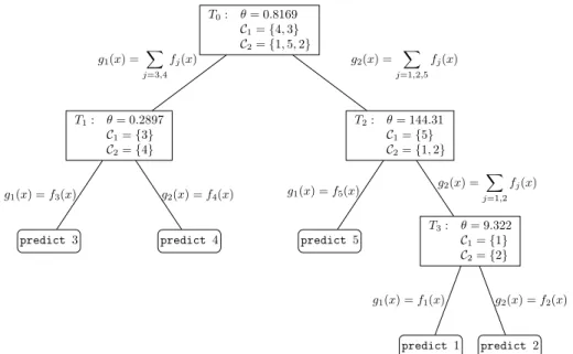
Fig. 1 Example run ofMetaClasson Nursery, a 5-class problem
example into a set of classes. Formally, we need a functionc:C×2C→R+. There are numerous natural extensions fromc toc. For our experiments, c represents the average cost of misclassifying instances into metaclasses inC1andC2. More formally, ifC⊆C, we
definec(y,C)to be 0 ify∈C(that is,x’s true label class is in the metaclass) and 1
|C|
j∈C
c(y, j )
otherwise. TheMetaClassalgorithm is presented as Algorithm 1.
Figure1gives an example of a tree built by theMetaClassalgorithm on the UCI (Blake and Merz2005) data set Nursery, a 5-class data set. At the root, the classes are divided into two metaclasses, each with about the same number of training examples represented in their respective classes. In this case, the thresholdθ=0.8169 favors the sum of confidences in metaclassC1= {4,3}as an optimal weight.
Predictions for a new examplex are made as follows. Starting at the root node, we tra-verse the tree towards a leaf. At each nodeT we compute the sum of confidences ofxwith respect to each associated metaclass. We traverse left or right down the tree depending on whetherg1(x)/g2(x)≥θ. When a leaf is reached, a final class prediction is made.
The number of nodes created byMetaClassis(n), wherenis the number of classes. Since the split into two metaclasses ensures each has an equal number of classes,MetaClass
results in a log(n)-depth tree. At each level, the most complex step is sorting at mostm instances according to the confidence ratio. Thus, the overall time complexity is bounded byO(mlog(m)log(n)). This represents a speedup to the algorithm of Lachiche and Flach (2003), which requires(nmlog(m))time. Classification is also efficient. At each node we compute a sum over an exponentially shrinking number of classes. The overall number of
Input: A set of instances,S= {x1, . . . , xm}; a set of classes,C= {1, . . . , n}; a learned confidence functionf:S×C→R+and a tree nodeT
Output: A decision tree with associated weights. if|C| =1 then
1
Stop, create a decision node and predict the class inC 2
end
3
SplitCinto two metaclassesC1,C2such that each metaclass has about an equal
4 number of classes. foreach Instancexi∈Sdo 5 g1(xi)= j∈C1fj(xi) 6 g2(xi)= j∈C2fj(xi) 7 G(xi)=g1(xi)/g2(xi) 8 end 9
Sort instances according toG 10
Select a thresholdθ that minimizes 11 m i=1 c(yi, Mθ(xi)) where Mθ(xi)= C1 ifθ≥G(xi) C2 otherwise LabelT withθ,C1,C2 12
Create two children ofT:Tleft, Tright
13
SplitSinto two sets, 14
S1= {xi∈S|Mθ(xi)=C1} S2= {xi∈S|Mθ(xi)=C2} Recursively perform this procedure onS1,C1, TleftandS2,C2, Tright
15 Algorithm 1:MetaClass operations is thus log(n)−1 i=0 n 2i,
which is linear in the number of classes: (n). This matches the time complexity of Lachiche and Flach’s with respect to classification.
6 Experimental results
The following experiments were performed on 24 UCI data sets (Blake and Merz2005), using Weka’s naïve Bayes (Witten et al.2005) as the baseline classifier and Matlab’s op-timization functions for reopop-timization. We ran experiments evaluating improvements both in classification accuracy and under non-uniform costs. We used 10-fold cross validation
for the error rate experiments. For the cost experiments, 10-fold cross validations were per-formed on 10 different cost matrices for each data set. Costs were integer values between 1 and 10, assigned uniformly at random. Costs on the diagonal were set to zero.
We evaluated the performance of each heuristic both in how well it was able to optimize the given cost function as well as how well the resultant classifier was able to generalize. To this end, we present performance on the training set as well as the testing set. Results for the optimization performance can be found in Table1while results for generalization can be found in Table2. In each table, results for the uniform (error rate) and non-uniform cost models can be found in subtables (a) and (b) respectively. For uniform cost, the average over the 10 folds is reported while for non-uniform costs, the average over all folds and cost matrices is reported. Thus, the values for non-uniform costs represent the average cost over all 100 experiments per data set, per algorithm.
In all tables, for each data set,ndenotes the number of classes whilemdenotes the total number of instances in each data set. The first column is the performance of our baseline classifier. For comparison, we have included results of our implementation for the algorithm of Lachiche and Flach (2003) on this baseline classifier (labeled “LF” in the tables). The re-sults of the experiments on our heuristics can be found in the last five columns of each table. Here, “MC” is theMetaClassalgorithm (Algorithm 1). “LP” is a linear programming solver (MOSEK ApS2005) on (21) withη=10−6. “GA1” is the sum of linear fractional
func-tions formulation (22) using a genetic algorithm. “GA2” is a genetic algorithm optimization of (1). Both experiments used the GA implementation from Abramson (2005). Parameters for both used the default Matlab settings with a population size of 20, a maximum of 200 generations and a crossover fraction of 0.8. The algorithm terminates if no change is ob-served in 100 continuous rounds. In addition, the mutation function of Abramson (2005) is guaranteed to only generate feasible solutions (in our case, all weights must be nonnegative). Upon termination, a direct pattern search is performed using the best solution from the GA. The final column is the quadratic program (QP) from Sect.5.1.3using the CVX software package (Grant et al.2006).
For all columns, values in italics indicate a worse performance than the baseline. En-tries in bold indicate a significant difference from the baseline with at least a 95% confi-dence according to a Student’stmethod. The overall best classifier(s) for each data set are underlined. Finally, the number of wins/losses (i.e. better/worse than the baseline) and those that are significant are summarized in each column. A win indicates that the heuristic im-proved upon the baseline while a loss indicates that the heuristic performed worse than the baseline.
To measure how well each algorithm is able to optimize, it would be ideal to compare it against an optimal solution. To do this, we could compute the optimal reweighting function either by solving the integer linear program of (9) or by running the constant-class algo-rithm presented in Sect.4. Unfortunately, neither of these options is feasible. Even forn=3 class data sets, the large number of instances forces an unmanageable number of variables in the ILP formulation (likewise for the constant-class algorithm). Even the best ILP pack-ages cannot handle such large numbers of variables. In lieu of such comparisons, we instead report the performance of each heuristic on the training set (Table1). That is, we report how well the heuristic was able to optimize the given problem. For data sets withn=2, the algorithm of Lachiche and Flach (2003) andMetaClassare optimal since they simplify to the two-class ROC threshold problem. However, in some instances, their performances differ slightly. This is due to rounding errors and how each implementation deals with bor-derline examples, thus the differences are negligible (in particular, the largest discrepancies correspond to at most 11 instances over all 10 folds being classified differently by the two algorithms).
Table 1 Optimization Performance. The two tables present the performance rates of each heuristic. Italicized
entries indicate the heuristic performed worse than the baseline (naïve Bayes) while non-italicized entries indicate an improvement or tie. A bold entry indicates a statistically significant difference from the baseline according to a Student’st-test with a 95% confidence level. For each data set, the overall best performing heuristic(s) are underlined
Data Set n m Naïve LF MC LP (21) GA1 (22) GA2 (1) QP Bayes
(a) Error rates. The values in this table represent performance under a uniform cost model
Audiology 24 226 0.2143 0.0840 0.1425 0.1705 0.1145 0.1637 0.1754 Bridges 2 (material) 3 107 0.0757 0.0602 0.0405 0.0540 0.0882 0.0519 0.0570 Bridges 2 (rel-l) 3 107 0.1173 0.0778 0.0737 0.1069 0.1245 0.0747 0.1038 Bridges 2 (span) 3 107 0.0560 0.0508 0.0342 0.0570 0.0633 0.0321 0.0570 Bridges 2 (type) 6 107 0.1277 0.0904 0.1059 0.1277 0.1381 0.1090 0.1080 Bridges 2 (t-or-d) 2 107 0.0176 0.0124 0.0135 0.0218 0.0426 0.0124 0.0290 Car 4 1728 0.1291 0.0914 0.1024 0.1153 0.1639 0.0914 0.1158 Post-Op 3 1473 0.4830 0.4525 0.4666 0.4830 0.4805 0.4632 0.4693 Horse-colic (code) 3 368 0.2276 0.2173 0.2237 0.2276 0.2303 0.2149 0.2339 Horse-colic (surgical) 2 368 0.1657 0.1388 0.1370 0.1657 0.1497 0.1376 0.1515 Horse-colic (site) 63 368 0.2970 0.2161 0.2623 0.2844 0.2744 0.2412 0.2820 Horse-colic (subtype) 2 368 0.0000 0.0003 0.0000 0.0000 0.0000 0.0000 0.0000 Horse-colic (type) 8 368 0.0105 0.0048 0.0045 0.0090 0.0057 0.0072 0.0072 Credit 2 1000 0.2288 0.2245 0.2255 0.2288 0.2594 0.2245 0.2371 Dermatology 6 366 0.0094 0.0042 0.0048 0.0078 0.0072 0.0051 0.0069 Ecoli 8 336 0.1134 0.0886 0.0962 0.1150 0.1031 0.0988 0.1180 Flags 8 194 0.2147 0.1523 0.1597 0.2090 0.1626 0.1718 0.2044 Glass 7 214 0.4522 0.3073 0.3172 0.4532 0.3525 0.4076 0.4449 Mushroom 2 8124 0.0419 0.0176 0.0177 0.0367 0.0188 0.0176 0.0266 Image Segmentation 7 2310 0.1948 0.1642 0.1361 0.1946 0.1215 0.1574 0.1982
Solar Flare (common) 8 1066 0.2189 0.1695 0.1671 0.2198 0.1707 0.1810 0.2011
Solar Flare (moderate) 6 1066 0.0660 0.0337 0.0332 0.0660 0.0337 0.0439 0.0469
Solar Flare (severe) 3 1066 0.0277 0.0045 0.0044 0.0223 0.0046 0.0182 0.0124
Vote 2 435 0.0968 0.0878 0.0883 0.0968 0.0906 0.0888 0.1031
Win/Loss – 23/1 23/0 11/5 15/8 23/0 16/7
Significant Win/Loss – 21/0 22/0 7/1 14/5 22/0 13/5
(b) Non-uniform costs. The values in this table represent performance under a non-uniform cost model. Audiology 24 226 1.2300 0.6019 0.7500 0.9663 0.7969 0.7173 0.9345 Bridges 2 (material) 3 107 0.3943 0.3408 0.1755 0.2916 0.4556 0.2565 0.3030 Bridges 2 (rel-l) 3 107 0.6772 0.4741 0.3759 0.6149 1.1963 0.3675 0.5873 Bridges 2 (span) 3 107 0.3290 0.3057 0.1999 0.3639 0.6190 0.2065 0.3740 Bridges 2 (type) 6 107 0.6728 0.6261 0.4416 0.6549 1.0157 0.4936 0.6077 Bridges 2 (t-or-d) 2 107 0.0966 0.0554 0.0554 0.1297 0.4614 0.0604 0.1334 Car 4 1728 0.7481 0.5314 0.5924 0.6863 1.6442 0.5103 0.6577 Post-Op 3 1473 2.8495 2.5125 2.6544 2.9183 3.6382 2.5371 2.7441
Table 1 (Continued)
Data Set n m Naïve LF MC LP (21) GA1 (22) GA2 (1) QP Bayes Horse-colic (code) 3 368 1.2740 1.1439 1.1797 1.2730 1.4168 1.1571 1.2972 Horse-colic (surgical) 2 368 1.0887 0.8043 0.7882 1.0926 1.2983 0.8309 0.9050 Horse-colic (site) 63 368 1.6023 1.4509 1.3801 1.5358 1.8110 1.1268 1.5908 Horse-colic (subtype) 2 368 0.0000 0.0017 0.0000 0.0000 0.0000 0.0000 0.0000 Horse-colic (type) 8 368 0.0597 0.0208 0.0197 0.0485 0.0325 0.0418 0.0397 Credit 2 1000 1.2160 0.9356 0.9372 1.2943 2.1381 0.9500 1.0035 Dermatology 6 366 0.0619 0.1426 0.0255 0.0520 0.0729 0.0325 0.0573 Ecoli 8 336 0.6024 0.5646 0.4768 0.6381 0.9202 0.4738 0.6535 Flags 8 194 1.2387 0.9360 0.8617 1.2092 1.0459 0.8970 1.1554 Glass 7 214 2.7112 1.6253 1.7130 2.7215 3.1616 2.2020 2.6379 Mushroom 2 8124 0.1926 0.0962 0.0962 0.1746 0.1247 0.0995 0.1348 Image Segmentation 7 2310 1.0715 1.2418 0.6963 1.0705 1.0546 0.8422 1.0791
Solar Flare (common) 8 1066 1.2229 0.8574 0.9157 1.2277 1.1494 0.8971 1.1500
Solar Flare (moderate) 6 1066 0.4174 0.2128 0.2076 0.4164 0.2709 0.2412 0.2935
Solar Flare (severe) 3 1066 0.1657 0.0260 0.0249 0.1468 0.0663 0.0948 0.0732
Vote 2 435 0.4527 0.3314 0.3335 0.4527 0.5320 0.4148 0.4539
Win/Loss – 21/3 23/0 14/8 8/15 23/0 17/6
Significant Win/Loss – 19/1 23/0 7/5 7/14 22/0 12/2
6.1 Generalization
Another measure of learning algorithms is how well they generalize beyond the training set. Unfortunately, none of the heuristics has any generalization guarantees other than what can be derived via standard PAC analysis. All algorithms could be adapted to use a validation set as yet another heuristic to improve generalization and prevent over-fitting. However, none of these techniques has any provable guarantees. In general, proving such guarantees is quite difficult. Results for error rates (uniform costs) and non-uniform costs are reported in Tables2a and2b, respectively.
6.2 Comparison and analysis
The significant wins and loses presented in Tables1 and 2provide a good reference to how well each algorithm performs individually with respect to the baseline as well as how much of an improvement each algorithm was able to achieve. As far as the optimization task (performance on the training set) is concerned, LF, MC and GA2 all showed statistically significant improvement over the baseline classifier in all or almost all data sets for both classification error and under non-uniform costs. These three methods also had superior performance in both settings with respect to the generalization task (performance on the test set).
For a more rigorous analysis, we performed a Friedman rank test as suggested by Demšar (2006) to compare the relative performances of multiple algorithms across multiple data sets. The Friedman test is a non-parametric statistical test similar to the parametric repeated mea-sures ANOVA. It is especially applicable in this case since we cannot make any normality
Table 2 Generalization Performance. The two tables present the test error rates of each heuristic. Italicized
entries indicate the heuristic performed worse than the baseline (naïve Bayes) while non-italicized entries indicate an improvement or tie. A bold entry indicates a statistically significant difference from the baseline according to a Student’st-test with a 95% confidence level. For each data set, the overall best performing heuristic(s) are underlined
Data Set n m Naïve LF MC LP (21) GA1 (22) GA2 (1) QP Bayes
(a) Error rates. The values in this table represent performance under a uniform cost model
Audiology 24 226 0.3094 0.2654 0.3227 0.2869 0.2826 0.2871 0.2737 Bridges 2 (material) 3 107 0.1581 0.2427 0.2527 0.2709 0.1763 0.2136 0.2436 Bridges 2 (rel-l) 3 107 0.3163 0.3527 0.3536 0.3081 0.3354 0.3454 0.3072 Bridges 2 (span) 3 107 0.2227 0.3290 0.3290 0.2427 0.4018 0.2799 0.2518 Bridges 2 (type) 6 107 0.4563 0.5499 0.4854 0.4654 0.4663 0.4654 0.4936 Bridges 2 (t-or-d) 2 107 0.1754 0.2418 0.2045 0.1754 0.1936 0.2499 0.1654 Car 4 1728 0.1464 0.1191 0.1249 0.1336 0.1723 0.1209 0.1331 Post-Op 3 1473 0.4948 0.4745 0.4833 0.4948 0.4989 0.4908 0.4853 Horse-colic (code) 3 368 0.3172 0.3148 0.3125 0.3172 0.2930 0.3120 0.3174 Horse-colic (surgical) 2 368 0.2089 0.1737 0.1764 0.2089 0.1791 0.1791 0.1980 Horse-colic (site) 63 368 0.7634 0.7770 0.7798 0.7634 0.7443 0.7660 0.7661 Horse-colic (subtype) 2 368 0.0027 0.0081 0.0081 0.0027 0.0027 0.0027 0.0027 Horse-colic (type) 8 368 0.0409 0.0407 0.0380 0.0409 0.0326 0.0353 0.0326 Credit 2 1000 0.2490 0.2569 0.2560 0.2490 0.2720 0.2579 0.2530 Dermatology 6 366 0.0272 0.0245 0.0274 0.0273 0.0272 0.0165 0.0219 Ecoli 8 336 0.1516 0.1427 0.1545 0.1545 0.1639 0.1368 0.1637 Flags 8 194 0.3760 0.4013 0.4318 0.3707 0.3705 0.3807 0.3860 Glass 7 214 0.5235 0.3792 0.4264 0.5235 0.4259 0.4958 0.5008 Mushroom 2 8124 0.0419 0.0179 0.0179 0.0374 0.0192 0.0178 0.0272 Image Segmentation 7 2310 0.1974 0.1809 0.1497 0.1974 0.1259 0.1727 0.1999
Solar Flare (common) 8 1066 0.2363 0.1726 0.1745 0.2363 0.1707 0.1979 0.2176
Solar Flare (moderate) 6 1066 0.0731 0.0337 0.0346 0.0731 0.0337 0.0506 0.0497
Solar Flare (severe) 3 1066 0.0281 0.0056 0.0046 0.0234 0.0046 0.0206 0.0141
Vote 2 435 0.0964 0.1081 0.1104 0.0964 0.0941 0.0965 0.1056
Win/Loss – 14/10 11/13 6/5 13/9 14/9 13/10
Significant Win/Loss – 7/3 7/2 3/1 6/0 7/1 5/2
(b) Non-uniform costs. The values in this table represent performance under a non-uniform cost model Audiology 24 226 1.7719 1.6826 1.8207 1.6385 1.7245 1.5194 1.6877 Bridges 2 (material) 3 107 0.8610 1.2188 1.3630 1.4725 1.0059 1.2180 1.3585 Bridges 2 (rel-l) 3 107 1.9355 2.2336 1.9764 1.9002 2.5553 1.9875 1.9163 Bridges 2 (span) 3 107 1.1871 1.7075 1.6680 1.2930 1.9934 1.4490 1.3508 Bridges 2 (type) 6 107 2.4584 2.3840 2.3612 2.6020 2.7605 2.5219 2.7270 Bridges 2 (t-or-d) 2 107 0.9654 1.0452 0.9729 0.9568 1.0794 0.9704 0.8096 Car 4 1728 0.8483 0.6653 0.7414 0.8073 1.6665 0.6522 0.7558 Post-Op 3 1473 2.9242 2.6791 2.7872 2.9993 3.6611 2.7056 2.8282
Table 2 (Continued)
Data Set n m Naïve LF MC LP (21) GA1 (22) GA2 (1) QP Bayes Horse-colic (code) 3 368 1.7914 1.6302 1.7247 1.7863 1.7950 1.6988 1.7726 Horse-colic (surgical) 2 368 1.3787 1.0191 1.0221 1.3890 1.6364 1.0629 1.1576 Horse-colic (site) 63 368 4.0891 3.9570 4.1976 4.1083 4.2647 4.0809 4.1560 Horse-colic (subtype) 2 368 0.0113 0.0432 0.0432 0.0113 0.0113 0.0113 0.0113 Horse-colic (type) 8 368 0.2225 0.2281 0.2086 0.2172 0.1704 0.1969 0.1894 Credit 2 1000 1.3202 1.0458 1.0477 1.3950 2.1906 1.0531 1.0805 Dermatology 6 366 0.1743 0.2649 0.1375 0.1564 0.1775 0.1146 0.1166 Ecoli 8 336 0.8104 0.8903 0.8168 0.8765 1.2116 0.7678 0.9218 Flags 8 194 2.1590 2.3070 2.3673 2.1407 2.3013 1.9888 2.1644 Glass 7 214 3.1308 2.0044 2.2886 3.1301 3.4910 2.6720 2.9600 Mushroom 2 8124 0.1929 0.0993 0.0994 0.1783 0.1262 0.1031 0.1382 Image Segmentation 7 2310 1.0854 1.2809 0.7733 1.0854 1.0989 0.8951 1.0883
Solar Flare (common) 8 1066 1.3079 0.9174 0.9662 1.3199 1.1622 0.9843 1.2331 Solar Flare (moderate) 6 1066 0.4644 0.2210 0.2216 0.4628 0.2749 0.2651 0.3030
Solar Flare (severe) 3 1066 0.1682 0.0361 0.0340 0.1556 0.0800 0.1069 0.0838
Vote 2 435 0.4510 0.3786 0.3699 0.4510 0.5346 0.4577 0.4605
Win/Loss – 14/10 15/9 12/9 6/17 17/6 15/8
Significant Win/Loss – 9/2 10/1 1/4 4/9 10/1 8/1
assumptions over dissimilar data sets from dissimilar domains. In each table (uniform/non-uniform cost on the train/test sets) for each data set, algorithms are ranked 1–7 based on their performance. A mean rank is taken for each algorithm and used to determine if some subset of algorithms is statistically significantly better than others. With a 95% confidence level, we can reject the hypothesis that all algorithms are equivalent for all four scenarios. That is, we can conclude that some set of algorithms outperform other methods with a high degree of certainty. Specific rankings can be found in Table3.
We also performed a post-hoc analysis using a Tukey-Kramer pairwise test (Hochberg and Tamhane1987). The results of this analysis can be found in Fig.2. For each table, the pairwise Tukey-Kramer test induces a partial order among the heuristics such that a relation from algorithmAto algorithmB (indicated by a directed edge A→B) implies thatAstatistically significantly outperformsB. Transitive relations are implicit so that if AoutperformsB andB outperformsC, thenAalso outperformsC. If no relation exists between two heuristics, then there is no statistically significant difference between them.
Following the post-hoc analysis, we can conclude that both greedy methods (MetaClass
and the algorithm of Lachiche and Flach2003) and the second genetic algorithm formulation (GA2) are consistently the top three performers. Only in the case of uniform cost in the generalization setting does the first genetic algorithm outperform GA2. However they are not statistically significantly different. Moreover, with respect to the optimization task in both cost settings (as well as the non-uniform cost generalization), all three algorithms are statistically significantly better than all other methods.
A case can now be made for preferring the simple greedy methods over the genetic algo-rithm. First, in all instances, one of the greedy methods either outperforms or is not statisti-cally significantly worse than GA2. In fact, it is never the case that GA2 statististatisti-cally
signifi-Table 3 Mean ranks. For each
data set, a rank 1–7 is assigned to algorithms according to their performance. The table lists the mean rank for each algorithm over all data sets for the optimization/generalization problems in the
uniform/non-uniform cost settings. The overall rank within each column is shown in parentheses
Algorithm Training Testing
Error Cost Error Cost
NB 5.7604 (7) 5.4167 (6) 4.4875 (7) 4.4250 (5) LF 2.1771 (1) 2.6146 (3) 3.6542 (2) 3.3188 (2) MC 2.4604 (2) 1.8708 (1) 3.8354 (3) 3.3229 (3) LP 5.3125 (6) 5.1896 (5) 4.4583 (6) 4.7542 (6) GA1 4.4146 (4) 5.7562 (7) 3.6292 (1) 5.0896 (7) GA2 2.8750 (3) 2.4979 (2) 3.8458 (4) 3.1292 (1) QP 5.0000 (5) 4.6542 (4) 4.0896 (5) 3.9604 (4)
(a) Error - Optimization. (b) Non-uniform Cost - Optimization.
(c) Error - Generalization. (d) Non-uniform Cost - Generalization.
Fig. 2 Relative performances. An arrow from algorithmAtoBindicatesAwas statistically significantly better thanB. Transitive relations are implicit. Statistics are according to a Tukey-Kramer pairwise compari-son with a 95% confidence level
cantly outperforms either of the two greedy methods. Second,MetaClassand the algorithm of Lachiche and Flach were both light on computational resources. Each fold required only a few seconds to execute for both algorithms. In contrast, the genetic algorithm (as well as all other methods) were extremely computation-intensive, requiring several minutes of
execution time. In addition, the genetic algorithm required a large number of generations; terminating the GA early resulted in poor performance. Thus, the greedy methods that used local decisions were just as good, and in most cases performed better, than the more sophis-ticated methods.
We can also make a similar, though less strong, case for preferringMetaClassover the algorithm of Lachiche and Flach. Though both performed very well, in most cases their performance was statistically equivalent. However, for the non-uniform cost optimization task, MetaClass statistically significantly outperformed LF. Though the time complexity ofMetaClass is faster than the algorithm of Lachiche and Flach, the data sets we used did not contain a large enough number of classes for the speed to become a significant advantage. However, in applications where the number of classes is large, this might become a significant issue. In addition, while both have similar resource requirements, the design of
MetaClassis arguably more flexible. First,MetaClasslearns what is essentially a decision tree, which is a provably more expressive hypothesis than a linear reweighting function. Any linear function can always be realized by a decision tree, but the converse is not true. Second, the choice of how we divide into separate metaclasses also gives us greater control over the learning process. In particular, since we can constrain the structure of the decision tree, we can customize to fit a specific learning domain using prior information. For instance, such an approach may fit well with hierarchical-class problems where we are given say, a taxonomy (i.e. an existing tree structure), and simply have to learnMetaClass’s parameters.
7 Conclusions
Reoptimizing an already-learned classifierf is an important problem in machine learning, particularly in applications where the cost model or class distribution of a learning problem deviates from the conditions under which a classifierfwas trained and the original training data forf is unavailable. We answered the open problem concerning the hardness of this reoptimization problem by showing that the decision version isNP-complete. Though im-practical, we also presented an algorithm that produces an optimal solution in polynomial time when the number of classes is constant. We also presented multiple algorithms for the multi-class version of this problem. Our experimental results showed that the greedy algo-rithms (ourMetaClassalgorithm and the algorithm of Lachiche and Flach2003) and one of our genetic algorithm approaches were roughly equally successful in reoptimizing under both uniform and non-uniform cost models. We found that, despiteMetaClass’s faster time complexity, in our experiments the number of classes was not large enough to give it a sig-nificant speed advantage. However, we also argued thatMetaClasshas several advantages over the algorithm of Lachiche and Flach in terms of its more expressive hypothesis class (trees) and its flexibility in partitioning the classes into metaclasses (e.g. in hierarchical clas-sification settings). Future work is to precisely identify contexts in which these advantages can be exploited.
There are several other avenues for future research. In the non-uniform cost setting, our methodology omitted extreme skews in costs between classes. It may be of interest to exam-ine such settings to see if the poor performing algorithms are able show improvement and to see if the better, greedy approaches continue to perform well. It would also be of interest to see if the greedy algorithms’ relative performance holds when we change the base clas-sifier. Do the greedy approaches still dominate if the base classifier is a more sophisticated learning algorithm like an SVM?
Finally, it is entirely possible that a better and more practical algorithm exists for the constant class setting. If so, how does its performance compare to the other methods?