The Stata Journal
EditorH. Joseph Newton Department of Statistics Texas A & M University College Station, Texas 77843 979-845-3142 979-845-3144 FAX [email protected] Executive Editor Nicholas J. Cox Department of Geography University of Durham South Road
Durham City DH1 3LE United Kingdom [email protected] Associate Editors Christopher Baum Boston College Rino Bellocco Karolinska Institutet David Clayton
Cambridge Inst. for Medical Research Charles Franklin
University of Wisconsin, Madison Joanne M. Garrett
University of North Carolina Allan Gregory
Queen’s University James Hardin
Texas A&M University Stephen Jenkins
University of Essex Jens Lauritsen
Odense University Hospital
Stanley Lemeshow Ohio State University J. Scott Long
Indiana University Thomas Lumley
University of Washington, Seattle Marcello Pagano
Harvard School of Public Health Sophia Rabe-Hesketh
Inst. of Psychiatry, King’s College London J. Patrick Royston
MRC Clinical Trials Unit, London Philip Ryan
University of Adelaide Jeroen Weesie
Utrecht University Jeffrey Wooldridge
Michigan State University
Copyright Statement:The Stata Journal and the contents of the supporting files (programs, datasets, and help files) are copyright cby Stata Corporation. The contents of the supporting files (programs, datasets, and help files) may be copied or reproduced by any means whatsoever, in whole or in part, as long as any copy or reproduction includes attribution to both (1) the author and (2) the Stata Journal.
The articles appearing in the Stata Journal may be copied or reproduced as printed copies, in whole or in part, as long as any copy or reproduction includes attribution to both (1) the author and (2) the Stata Journal.
Written permission must be obtained from Stata Corporation if you wish to make electronic copies of the insertions. This precludes placing electronic copies of the Stata Journal, in whole or in part, on publically accessible web sites, fileservers, or other locations where the copy may be accessed by anyone other than the subscriber.
Users of any of the software, ideas, data, or other materials published in the Stata Journal or the supporting files understand that such use is made without warranty of any kind, by either the Stata Journal, the author, or Stata Corporation. In particular, there is no warranty of fitness of purpose or merchantability, nor for special, incidental, or consequential damages such as loss of profits. The purpose of the Stata Journal is to promote free communication among Stata users.
TheStata Technical Journal, electronic version (ISSN 1536-8734) is a publication of Stata Press, and Stata is a registered trademark of Stata Corporation.
The Stata Journal (2002)
2, Number 3, pp. 280–289
Comparative assessment of three common
algorithms for estimating the variance of the
area under the nonparametric receiver
operating characteristic curve
Mario A. Cleves, Ph.D.
Arkansas Center for Birth Defects Research and Prevention Department of Pediatrics, University of Arkansas for Medical Sciences
Little Rock, Arkansas
Abstract. The area under the receiver operating characteristic (ROC) curve is often used to summarize and compare the discriminatory accuracy of a diagnostic test or modality, and to evaluate the predictive power of statistical models for binary outcomes. Parametric maximum likelihood methods for fitting of theROC curve provide direct estimates of the area under theROCcurve and its variance. Nonparametric methods, on the other hand, provide estimates of the area under the ROC curve, but do not directly estimate its variance. Three algorithms for computing the variance for the area under the nonparametricROCcurve are com-monly used, although ambiguity exists about their behavior under diverse study conditions. Using simulated data, we found similar asymptotic performance be-tween these algorithms when the diagnostic test produces results on a continuous scale, but found notable differences in small samples, and when the diagnostic test yields results on a discrete diagnostic scale.
Keywords: st0020, receiver operating characteristic (ROC) curve, trapezoidal rule, sensitivity, specificity, discriminatory accuracy, predictive power
1
Introduction
The discriminatory accuracy of a diagnostic test or classification method is frequently evaluated by its ability to correctly classify subjects into disease states. The receiver operating characteristic (ROC) curve, a plot of the diagnostic test’s sensitivity versus 1−specificity at the various observed values of the test, can be used to quantify the accuracy with which the diagnostic test can discriminate between two states or condi-tions. TheROCcurve is also useful in assessing the predictive and discriminatory power of statistical models for binary outcomes (Hosmer and Lemeshow 2000), and specifi-cally, it has been used to assess the predictive power of competing comorbidity indices computed from administrative data (Cleves et al. 1997).
The overall discriminatory power of a diagnostic test is commonly summarized by the area under theROCcurve (AUC). Assuming that higher values of a diagnostic test are associated with “abnormal” subjects, while lower values are associated with “normal” subjects, then the AUC is interpretable as the probability that the observed value of
c
the diagnostic test will be greater for a randomly selected abnormal subject than for a randomly selected normal subject (DeLong et al. 1988). Thus, the greater theAUC, the better the overall discriminatory power of the diagnostic test or statistical model.
Both nonparametric and parametric methods for fitting theROCcurve and estimat-ing its area have been developed and implemented in Stata’s rocsuite of commands. Parametric techniques are based on the assumption that there is an unobserved contin-uous latent variable with known distribution in both the normal and abnormal popula-tions, and based on this assumption, a smooth maximum likelihoodROCcurve is fitted to the observed data. TheAUCand its variance are then computed directly as functions of the estimated maximum likelihood parameters of the fitted curve (Dorfman and Alf 1969). See [R]rocfor a complete description of these commands.
By contrast, nonparametric methods require no assumption about the existence or the distributional form of an unobserved continuous latent variable. They simply compute theAUCbased on the ROCpoints. The method implemented in Stata simply connects the points on theROCcurves using straight lines, and computes theAUCusing the trapezoidal rule. Nonparametric methods for estimating theAUC, however, do not yield variance estimates for theAUC. Estimates of the variance for the area under the
nonparametricROCcurve are computed in Stata using one of three popular algorithms:
the first suggested byBamber in 1975, the second suggested by Hanley and McNeilin 1982, and the third suggested byDeLong et al.in 1988.
The DeLong, DeLong, and Clarke-Pearson method was selected as the default be-cause in several scenarios examined by the author it seemed to perform better than the other two methods (Cleves 1999). It is unclear, however, if there are any general systematic differences between these estimators. In an attempt to answer this question, we examine the performance of these three algorithms for computing the area under the
ROCcurve under various simulated conditions.
2
Methods
2.1
Algorithms for computing variance for the area under the ROC
curve
Although much of this information is found in the Stata manual, for completeness, we review in this section the three algorithms for computing the variance for the area under theROCcurve.
Assume, without loss of generality, that higher values of a diagnostic test are as-sociated with “abnormal” subjects, while lower values are asas-sociated with “normal” subjects. Further, assume that the diagnostic test is applied to Nn normal and Na abnormal subjects. Let Xi, i = 1,2, . . . , Na and Yi, j = 1,2, . . . , Nn be the observed outcomes of the diagnostic test for the abnormal and normal subjects, respectively, and letθbe the nonparametric estimate of the area under theROCcurve.
282 Variance of the area under the nonparametric ROC curve
in 1975. He showed that theAUC, when calculated using the trapezoidal rule, is equal to the Mann–Whitney U-statistic and provided an algorithm for estimating its variance.
Define for any two Y values, Yj and Yk, and any Xi value,
byyx=p(Yj,Yk <Xi) +p(Xi<Yj,Yk)−2p(Yj <Xi<Yk)
and similarly, define for any two values of two X values, Xi and Xl, and any Yj value,
bxxy=p(Xi,Xl<Yj) +p(Yj <Xi,Xl)−2p(Xi<Yj <Yl)
Then, Bamber’s unbiased estimate of the variance for theAUCis computed as var(θ) =14(Na−1)(Nn−1)∗
p(Xi= Y) + (Na−1)bxxy+ (Nn−1)byyx−4(Na+Nn−1)(θ−0.5)2
The second algorithm was described byHanley and McNeilin 1982. For brevity, we will refer to this as Hanley’s method. Hanley’s variance for the AUC is computed as follows. Let Q1 be the probability that two randomly selected abnormal subjects will both have a higher score than a randomly selected normal subject, and let Q2 be the probability that one randomly selected abnormal subject will have a higher score than any two randomly selected normal subjects. Then, the variance for theAUCderived by
Hanley and McNeil is computed as
var(θ) = θ(1−θ) + (Na−1)(Q1−θ 2) + (N
n−1)(Q2−θ2)
NnNa
The most recent of the three algorithms was suggested byDeLong et al.(1988); we will refer to this as DeLong’s method. Their method was derived in the context of developing an approach for comparing areas under two or moreROCcurves. They sug-gested using a comparison variance–covariance matrix computed based on Sen’s (1960) structural components method for obtaining the elements of the variance–covariance matrix of a vector of U-statistics. The variance of each of the areas under the curve is obtained as the corresponding diagonal element of the computed variance–covariance matrix.
The DeLong variance for eachAUCis computed as follows. Define for each abnormal subject,i, the quantities
V10(Xi) = 1 Nn Nn j=1 ψ(Xi,Yj) and S10= 1 Na−1 Nn i=1 V01(Xi)−θ 2
and similarly, define for each normal subject,j, the quantities
V01(Yj) = 1 Na Na i=1 ψ(Xi,Yj) and S01= 1 Nn−1 Nn j=1 V01(Yj)−θ 2
where ψ(Xi,Yj) = 1 Y<X 1 2 Y = X 0 Y>X Then, DeLong’s variance of the estimatedAUCis given by
var(θ) = 1
NaS10 + 1
NnS01
2.2
Simulations
Data were simulated by assuming both a diagnostic test that produced results in a continuous scale, such as blood pressure or serum glucose level, and a diagnostic test that produced results in an ordinal scale similar to those produced by rating or ranking modalities.
In all cases, data were simulated assuming the existence of an unobserved latent variable that is Gaussian distributed in both the “normal” and “abnormal” subpopu-lations. For each simulation, a random sample of predetermined size was drawn from each of these subpopulations. When the diagnostic test was assumed to produce results on a continuous scale, the randomly selected value was directly used in theROC compu-tations. When the diagnostic test was assumed to produce results in the ordinal scale, the complete population was first partitioned into a predetermined number of discrete categories (4, 6, or 8). Each randomly selected continuous observation was then recoded to the discrete value corresponding to the value of the category in which the observation fell.
Data were simulated for sample sizes of 10, 25, 50, 100, and 150 observations per group. The degree of overlap of the two populations was controlled by generating observations from Gaussian distributions whose means differed by 0.5, 1, 1.5, 2.0, and 2.5 standard deviations. Additionally, data were simulated assuming equal variances in the two subpopulations, and assuming distributions with standard deviation ratios of 1:1.5, 1:2 and 1:2.5. Each of the 100 combination of sample size, degree of overlap, and standard deviation ratio was replicated 5,000 times.
From each of the 5,000 replications, the area under theROC curve was calculated using the trapezoidal rule, and three variances were computed using the previously described algorithms. Thus, each simulation generated 5,000 areas and 15,000 variance estimates (5,000 from each of the three methods). For each simulation, the empirical standard deviation of the AUC was computed as the standard deviation of the 5,000 areas under the curve.
For each simulation, comparisons were made by subtracting the computed aver-age standard deviation of each method from the empirical standard deviation. Thus, positive differences indicate an estimated standard deviation less than the empirical standard deviation (i.e., an underestimation of the empirical value), while a negative difference indicates an overestimation of the empirical standard deviation.
284 Variance of the area under the nonparametric ROC curve
3
Results
3.1
Continuous scale
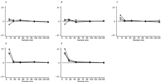
Plotted in Figure 1 are the results of simulations assuming a diagnostic test that pro-duced results in a continuous scale from two normal populations with equal standard deviations. Similarly, Figure 2 summarizes results from simulations also assuming a diagnostic test that produced results in a continuous scale, but from two normal pop-ulations with unequal standard deviations of 1:2. Results assuming other standard deviation ratios were similar to these, and thus are not presented here. In these and all subsequent graphs, a horizontal line at zero is plotted for reference. Data points above this reference line indicate an underestimation of the empirical standard deviation, while data points below the reference line indicate an overestimation of the empirical standard deviation. A Sample size 0 15 30 45 60 75 90 105 120 135150 −.01 0 .01 B Sample size 0 15 30 45 60 75 90 105 120 135150 −.01 0 .01 C Sample size 0 15 30 45 60 75 90 105 120 135150 −.01 0 .01 D Sample size 0 15 30 45 60 75 90 105 120 135150 −.01 0 .01 E Sample size 0 15 30 45 60 75 90 105 120 135150 −.01 0 .01
Figure 1: Results of simulations assuming a diagnostic test that produces measure-ments on a continuous scale from a binormal population with equal standard deviations. Graphs A through E are for populations with means 0.5, 1.0, 1.5, 2.0, and 2.5 standard deviations apart, respectively. ◦-Delong,2-Hanley, and-Bamber
A Sample size 0 15 30 45 60 75 90 105 120 135150 −.01 0 .01 B Sample size 0 15 30 45 60 75 90 105 120 135150 −.01 0 .01 C Sample size 0 15 30 45 60 75 90 105 120 135150 −.01 0 .01 D Sample size 0 15 30 45 60 75 90 105 120 135150 −.01 0 .01 E Sample size 0 15 30 45 60 75 90 105 120 135150 −.01 0 .01
Figure 2: Results of simulations assuming a diagnostic test that produces measurements on a continuous scale from a binormal population with unequal standard deviations of 1:2 ratio. Graphs A through E are for populations with means 0.5, 1.0, 1.5, 2.0, and 2.5 standard deviations apart, respectively. ◦-Delong,2-Hanley, and-Bamber
For sample sizes of 25 or greater, all three algorithms produced similar results close to the empirically expected value. They all approached the expected value as the sample size, and the distance between populations increased.
Some variability in the estimation, however, was noted for smaller samples, with a tendency of the three methods to underestimate the empirical standard deviation as the distance between the populations increased. No single method consistently outper-formed another in these simulations.
3.2
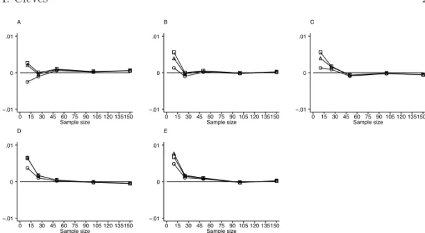
Discrete ordinal scale
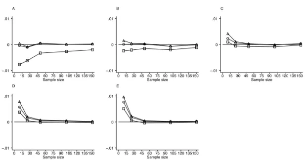
Summarized in Figure 3 are the results of simulations assuming a diagnostic test that produced results at four values of a discrete ordinal scale from two normal populations with equal standard deviations. Similarly, Figure 4 summarizes results from simulations also assuming a diagnostic test that produced results at four values of a discrete ordinal scale, but from two normal populations with unequal standard deviations of 1:2. Results assuming four result categories and other standard deviation ratios were similar to these, and thus are not presented here. The standard deviations estimated by the DeLong and Bamber algorithm produced similar results. As with the continuous outcome scale, they produced results close to the empirically expected value for sample sizes larger than 25. They also produced results close to the empirically expected value when the population means were less than 1.5 standard deviations apart. However, they underestimated the empirical standard deviation as the distance between the populations increased.
286 Variance of the area under the nonparametric ROC curve A Sample size 0 15 30 45 60 75 90 105 120 135150 −.01 0 .01 B Sample size 0 15 30 45 60 75 90 105 120 135150 −.01 0 .01 C Sample size 0 15 30 45 60 75 90 105 120 135150 −.01 0 .01 D Sample size 0 15 30 45 60 75 90 105 120 135150 −.01 0 .01 E Sample size 0 15 30 45 60 75 90 105 120 135150 −.01 0 .01
Figure 3: Results of simulations assuming a diagnostic test that produces results at 4 values of a discrete ordinal scale from a binormal population with equal standard deviations. Graphs A through E are for populations with means 0.5, 1.0, 1.5, 2.0, and 2.5 standard deviations apart, respectively. ◦-Delong,2-Hanley, and-Bamber
A Sample size 0 15 30 45 60 75 90 105 120 135150 −.01 0 .01 B Sample size 0 15 30 45 60 75 90 105 120 135150 −.01 0 .01 C Sample size 0 15 30 45 60 75 90 105 120 135150 −.01 0 .01 D Sample size 0 15 30 45 60 75 90 105 120 135150 −.01 0 .01 E Sample size 0 15 30 45 60 75 90 105 120 135150 −.01 0 .01
Figure 4: Results of simulations assuming a diagnostic test that produces results at 4 values of a discrete ordinal scale from a binormal population with unequal standard deviations of 1:2 ratio. Graphs A through E are for populations with means 0.5, 1.0, 1.5, 2.0, and 2.5 standard deviations apart, respectively.◦-Delong,2-Hanley, and-Bamber On the other hand, Hanley’s method consistently produced standard deviations greater than the other two methods, in most cases overestimating the empirical standard deviation. Hanley’s method, however, approached the results of the other two methods and the empirical value as either the sample size or the distance between populations increased.
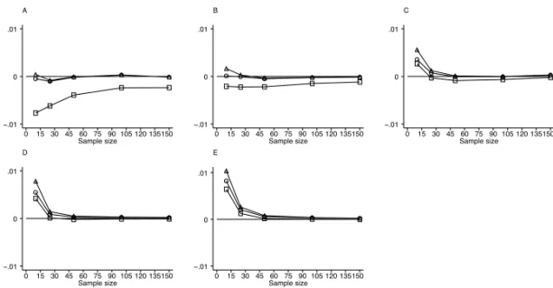
All three methods underestimated the standard deviation for small sample sizes when the distance between populations exceeded one standard deviation. This underes-timation became more pronounced as the distance between the populations increased. Similar results were observed when data were simulated assuming six and eight classi-fication levels (Figure 5).
A Sample size 0 15 30 45 60 75 90 105 120 135150 −.01 0 .01 B Sample size 0 15 30 45 60 75 90 105 120 135150 −.01 0 .01 C Sample size 0 15 30 45 60 75 90 105 120 135150 −.01 0 .01 D Sample size 0 15 30 45 60 75 90 105 120 135150 −.01 0 .01 E Sample size 0 15 30 45 60 75 90 105 120 135150 −.01 0 .01
Figure 5: Results of simulations assuming a diagnostic test that produces results at 8 values of a discrete ordinal scale from a binormal population with equal standard deviations. Graphs A through E are for populations with means 0.5, 1.0, 1.5, 2.0, and 2.5 standard deviations apart, respectively. ◦-Delong,2-Hanley, and-Bamber
4
Conclusions
The area under the receiver operating characteristic (ROC) curve has been successfully used to summarize and compare the discriminatory accuracy of a diagnostic test and to evaluate the predictive power of statistical models for binary outcomes (Harrell et al. 1984). When this area is computed nonparametrically, three algorithms for computing its variance are commonly used. These three methods were compared by simulating data under various conditions.
When the outcome of the diagnostic test was measured on a continuous scale, little difference was found between the methods for sample size greater than 30 in each of the “normal” and “abnormal” groups. Not unexpectedly, the estimates from all three meth-ods approached the empirically expected variance as the number of subjects per group increased. The more noticeable differences were found for smaller sample sizes, where all three methods yielded variances smaller than the empirically expected values and more variability between methods was found. Based on these simulations of continuous out-comes, it is difficult to recommend a single method, although DeLong’s method tended to yield values closer to expected in cases where the normal and abnormal population means were more than one standard deviation apart.
288 Variance of the area under the nonparametric ROC curve
When the outcome of the diagnostic test was measured on a discrete ordinal scale, the methods developed byDeLong et al.and by Bamber outperformed Hanley and Mc-Neil’s method. This was true regardless of sample size and distance between population means. The Hanley and McNeil’s method always yielded standard deviations that were greater than those of the other two methods and frequently produced values that were greater than the empirically expected value. Based on these simulations, statistical tests comparingROCareas constructed using Hanley and McNeil’s variance estimator will be overly conservative when a discrete rating scale such as a comorbidity index is used. This negative bias of the Hanley and McNeil’s method could be of concern. In particular this method is often used to compute sample sizes and could also potentially impact statistical inference, statistical power, and confidence interval coverage probabilities.
5
References
Bamber, D. 1975. The area above the ordinal dominance graph and the area below the receiver operating graph. Journal of Mathematical Psychology 12: 387–415.
Cleves, M. A. 1999. sg120: Receiver Operating Characteristic (ROC) analysis. Stata
Technical Bulletin 52: 19–33. InStata Technical Bulletin Reprints, vol. 9, 212–229. College Station,TX: Stata Press.
Cleves, M. A., N. Sanchez, and M. Draheim. 1997. Evaluation of two competing methods for calculating Charlson’s comorbidity index when analyzing short-term mortality using administrative data. Journal of Clinical Epidemiology 50: 903–908.
DeLong, E. R., D. M. DeLong, and D. L. Clarke-Pearson. 1988. Comparing the areas un-der two or more correlated receiver operating characteristic curves: A nonparametric approach. Biometrics44: 837–845.
Dorfman, D. D. and E. Alf, Jr. 1969. Maximum likelihood estimation of parameters of signal detection theory and determination of confidence intervals-rating method data. Journal of Mathematical Psychology 6: 487–496.
Hanley, J. A. and B. J. McNeil. 1982. The meaning and use of the area under a receiver operating characteristic (ROC) curve. Radiology 143: 29–36.
Harrell, F. E., Jr., K. L. Lee, R. M. Califf, D. B. Pryor, and R. A. Rosati. 1984. Regres-sion modelling strategies for improved prognostic prediction. Statistics in Medicine 3: 143–152.
Hosmer, D. W., Jr. and S. Lemeshow. 2000. Applied Logistic Regression. 2d ed. New York: John Wiley and Sons.
Sen, P. K. 1960. On some convergence properties of U-statistics. Calcutta Statistical Association Bulletin10: 1–18.
About the Author
Mario Cleves is an Associate Professor in the Department of Pediatrics at the University of Arkansas for Medical Sciences.