A Survey on Spectral-Spatial Classification
Techniques based on Attribute Profiles
Pedram Ghamisi,
Student Member, IEEE and
Mauro Dalla Mura,
Member, IEEE
Jon Atli Benediktsson,
Fellow, IEEE
Abstract—Just over a decade has passed since the concept
of morphological profile was defined for the analysis of remote sensing images. From that time, the morphological profile has largely proved to be a powerful tool able to model spatial information (e.g., contextual relations) of the image. However,
due to the shortcomings of using the morphological profiles, many variants, extensions and refinements of its definition have appeared stating that the morphological profile is still under continuous development. In this case, recently-introduced-theoretically-sound attribute profiles can be considered as a generalization of the morphological profile, which is a powerful tool to model spatial information existing in the scene. Although the concept of the attribute profile has been introduced in remote sensing only recently, an extensive literature on its use in different applications and on different types of data has appeared. To that end, the great amount of contributions in the literature that address the application of the attribute profile to many tasks (e.g.,
classification, object detection, segmentation, change detection, etc.) and to different types of images (e.g., panchromatic,
mul-tispectral, hyperspectral) proves how the attribute profile is an effective and modern tool. The main objective of this survey paper is to recall the concept of the attribute profiles along with all its modifications and generalizations with a special emphasize on remote sensing image classification and summarize the important aspects of its efficient utilization while also listing potential future works.
Index Terms—Spectral-spatial classification, attribute profile,
morphological attribute filters, spatial features, hyperspectral image analysis.
I. INTRODUCTION
S
UPERVISED classification is an important process in remote sensing image analysis. A wide range of appli-cations such as crop monitoring, forest appliappli-cations, urban development, mapping and tracking and risk management can be handled by using appropriate data and efficient classifiers. A large amount of data with different spectral, spatial and temporal resolutions is currently being made available for different applications. Hyperspectral imaging sensors are able to capture hundreds of narrow spectral channels with a very fine spectral resolution, which is helpful for detailed physical analysis of structures in the captured image [1]. In addition, thanks to recent advances in remote sensing technologies, spatial resolution of sensors is also improving [1], which has led to a better identification of relatively small structures.P. Ghamisi and J. A. Benediktsson are with the Faculty of Electrical and Computer Engineering, University of Iceland, 107 Reykjavik, Iceland (corresponding author, e-mail: [email protected]).
M. Dalla Mura is with Speech Signals and Automatics Laboratory (GIPSA-Lab) at Grenoble Institute of Technology (Grenoble INP), France.
This research was supported in part by the Icelandic Research Fund for Graduate Students and the program J. Verne 2014, projectn◦31936TD.
Conventional spectral classifiers consider the image as an ensemble of spectral measurements without exploiting their spatial arrangement. In other words, the spatial organization of distinct pixels is not considered in spectral classification [2]. In order to make use of the spatial organization, a joint spectral and spatial classifier is required to reduce the label-ing uncertainty that exits when only spectral information is taken into account. Furthermore, more spatially homogeneous classification maps are produced. Moreover, spatial informa-tion provides addiinforma-tional discriminant informainforma-tion related to the shape and size of different structures, which if properly exploited, leads to more accurate classification maps.
In order to model the spatial information of a scene, two common strategies are available: A crisp neighborhood system and an adaptive neighborhood system [1]. While the first one mostly relies on considering spatial and contextual dependen-cies in a predefined neighborhood system, the latter shows more flexibility and is not confined to a given neighborhood system.
One well-known way for extracting spatial information by using a crisp neighborhood system is the use of MRF modeling
1 (Please see the list of abbreviations shown in Fig. I). MRF
is a family of probabilistic models and can be explained as a 2-D stochastic process over discrete pixels lattices [3]. MRF is considered to be a powerful tool for incorporating spatial and contextual information into the classification framework [4]. There is a considerable literature on the use of MRFs in classification. For example, in [5], the result of the prob-abilistic SVM was regularized by an MRF. In [6], a fully automated framework for the spectral and spatial classification of hyperspectral (multispectral) data was proposed, which was based on the integration of a modification of MRF (Hidden MRF) and SVM. However, the main disadvantages of considering a set of crisp neighbors are that
1) the standard neighborhood system may not contain enough samples to characterize the object of interest, and this downgrades the effectiveness of the classifier (in particular, when the input data set is of high resolution and the neighboring pixels are highly correlated [1]) 2) a larger neighborhood system leads to intractable
com-putational problems [1].
In order to address the above-mentioned issues, an adaptive neighborhood system can be considered. One possible way for
1Please note that here we are discussing the most well-known MRF model,
which models the spatial information of adjacent pixels by considering a crisp neighborhood system. However, MRFs based on an adaptive neighborhood system can be found in literature as well.
TABLE I LIST OF ABBREVIATIONS.
VHR Very High Resolution MRF Markov Random Field SE Structuring Element MP Morphology Profile EMP Extended Morphology Profile DMP Differential Morphology Profile
AF Attribute Filter AP Attribute Profile MAP Multivariate Attribute Profile
EAP Extended Attribute Profile EMAP Extended Multivariate Attribute Profile EEMAP Entire Extended Multivariate Attribute
Profile SDAP Self-Dual Attribute Profile
SVM Support Vector Machine RF Random Forest MLR Multinomial Logistic Regression
SRC Sparse Representation Classification RBF Radial Basis Function
FS Feature Selection FE Feature Extraction PC Principal Component PCA Principal Component Analysis KPCA Kernel Principal Component Analysis
ICA Independent Component Analysis DAFE Discriminant Analysis Feature Extraction DBFE Decision Boundary Feature Extraction NWFE Nonparametric Weighted Feature Extraction
GA Genetic Algorithm PSO Particle Swarm Optimization BFODPSO Binary Fractional Order Darwinian Particle
Swarm Optimization GLCM Gray-Level Co-occurrence Matrix
considering the adaptive neighborhood system is to utilize dif-ferent types of segmentation methods. Segmentation of images into spatially homogenous regions may improve the accuracy of classification maps [7]. To make such an approach more effective, an accurate segmentation of the image is required [8]. There is an extensive literature on the use of segmentation techniques in order to extract the spatial information (e.g., [9–
12]).
Another possible set of approaches which are able to extract spatial information by using an adaptive neighborhood system relies on the concept of the MP. An MP is constructed based on the repeated use of openings and closings by reconstruction with a SE of an increasing size, applied to a scalar image. MPs simultaneously attenuate some spatial details and preserve the geometrical characteristics of the other regions. Pesaresi and Benediktsson [13] used morphological transformations to build the so-called MP. In [14], the MP generated by morphological opening and closing operations was used for classifying a Quickbird panchromatic image captured over Bam, Iran which was hit by the earthquake in 2003. To do so, the spatial features extracted by the MP were considered for assessing the damages caused by the earthquake. The standard opening and closing along with white and black top hat [15], and opening and closing by reconstruction were computed and the resulting features were classified using a SVM classifier for the classification of a Quickbird panchromatic image in [16]. An automatic hierarchical segmentation technique based on the analysis of the DMP (the derivative of the MP) was proposed in [17]. The DMP was also analyzed in [18], by extracting
a fuzzy measure of the characteristic scale and contrast of each structure in the image. The computed measures were compared with the possibility distribution predefined for each thematic class, generating a value of membership degree for each class used for classification. In [19], in order to reduce the dimensionality of data and address the so-called curse of dimensionality [20], feature extraction techniques were taken into consideration for the DMP classified by a neural network classifier. In [21], the concept of MPs was successfully ex-tended to handle hyperspectral images, resulting in the EMP. The EMP is obtained by first reducing the dimensionality of the hyperspectral image with a PCA and by computing an MP on each of its first few components.
Some studies have been conducted in order to assess the capability of SEs with different shapes for the extraction of spatial information. For instance, MPs computed with a compact SE (e.g., square, disk, etc.) can be considered for
modeling the size of the objects in the image (e.g., in [1]
this information was exploited to discriminate small buildings from large ones). In [22], the computation of two MPs was introduced in order to model both the length and the width of the structures. In more detail, one MP is built using disk-shaped SEs for extracting the smallest size of the structures, while the other employs linear SEs (which generate directional profiles [23]) for characterizing the object’s maximum size (along with the orientation of the SE). This is appropriate for defining the minimal and maximal length. However, such analysis is computationally intensive as all the possible lengths and orientations cannot be practically investigated. Also in [22], the authors proposed to use operators based on ”partial reconstruction” instead of the conventional geodesic recon-struction in order to reduce the ”leakage effect”. In [24], a new binary optimization method inspired on the Fractional-Order Darwinian Particle Swarm Optimization [8] is introduced in order to select the most informative features extracted by MP. Based on the above-mentioned literature, it is easy to infer that multiscale processing based on morphological filters (e.g., by MPs, DMPs and EMPs) has proven to be effective
in extracting informative spatial features from the images to be analyzed. Although MP is a powerful technique for the extraction of spatial information, the concept has a few limitations: i) the shape of SEs is fixed and ii) SEs are unable to characterize information related to the gray-level characteristics of the regions. To overcome this, the mor-phological AP has been proposed as the generalization of the MP which provides a multilevel characterization of an image by using the sequential application of morphological AF [25]. AFs are connected operators which process an image by considering only its connected components. For binary images, the connected components are simply the foreground and background regions present in the image. In order to deal with gray-scale images, the set of connected components can be obtained by considering the image to be composed by a stack of binary images generated by thresholding the image at all its grey-level values [26]. Thus, they process the image without distorting or inserting new edges but only by merging existing flat regions [15]. AFs were employed for modeling the structural information of the scene in order
to increase the effectiveness of a classification and building extraction in [25, 27], respectively, where they proved to be efficient for the modeling of structural information in VHR images. In [28], AFs were used in a scheme for building height retrieval by considering VHR images acquired on the same area with different acquisition angles. Namely, the filters were used for reducing the complexity of the images in order to isolate regions that corresponds to the rooftops of buildings. A neural network was used to find correspondences between the extracted regions in the different images by considering moment invariants descriptors as features. After finding correspondences and since the building considered had a flat roof, the horizontal displacement of matching regions was converted in height by trigonometry.
AFs include in their definition, the morphological operators based on geodesic reconstruction [29]. Moreover, AP is a flexible tool since images can be processed based on many different types of attributes. In fact, the attributes can be of any type. For example, they can be purely geometric, or related to the spectral values of the pixels, or on different characteristics such as spatial relations to other connected components. Furthermore, in [27], the problem of tuning the parameters of the filters was addressed by proposing an automatic feature selection procedure based on a genetic algo-rithms. In [30], it was proved that the automatic method with considering only two attributes (area and standard deviation) is comparative with manual technique with four attributes in terms of classification accuracy and CPU processing time. In [31], a topographic map of the image was used, which is autodual (it is invariant to contrast inversion) and does not require any SE in order to extract the profiles. In addition, the concept of MPs was extended to the profiles of other features (e.g., perimeters, scales, total variations).
This work presents a survey over the existing papers re-lated to AP with a special emphasize on multispectral and hyperspectral image classification, while still providing with a general framework for other types of data. The rest of this survey paper is organized as follows: first, a few primary concepts related to morphological profiles will be disscused in II. Then, the concept of AP and its extension for hyperspectral data will be explained in Section III. Then, Section IV is devoted to spectral and spatial classification of remote sensing data by considering AP. Section V is on the use of AP for other types of applications such as change detection and other types of data such as LiDAR. In Section VI, the main obtained points, advantages and disadvantages of different techniques as well as the survey of existing experiments with respect to classification results will be briefly discussed. Finally, Section VII outlines the main conclusions and possible future works.
II. MORPHOLOGICALPROFILE
In this section, first we recall a few primary concepts such
as connected components,basic morphological operatorsand
morphology profiles and its modifications.
A. Connected components
A connected component is regarded as a group of iso-level pixels which are connected according to a predefined connectivity rule. The most well-known connectivity rules are 4- and 8-connected, where a pixel is considered as adjacent to the four or eight of its neighboring pixels, respectively.
B. Basic morphological operators
Erosion and dilation are considered as the basic building blocks of mathematical morphology. These operations are carried out on an image with a set of known shape, called an SE. Opening and closing are combinations of erosion and dilation. These operators simplify the input data by removing structures with size less than the one of SE. However, they can influence on the shape of the structures and can introduce fake objects in the image [32]. One way to handle this issue is to consider opening and closing by reconstruction [15].
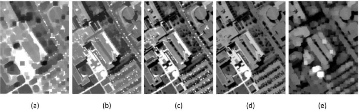
Opening and closing by reconstruction filters are a family of connected operators which satisfy the following criterion: If SE cannot fit in an object, then it will be totally removed, otherwise it will be totally preserved. Reconstruction operators remove objects smaller than SE without altering the shape of those objects and reconstruct connected components from the preserved objects. For gray-scale images, opening by reconstruction removes unconnected light objects and in dual, closing by reconstruction removes unconnected dark objects. Fig. 1 illustrates the different results that are obtained when considering operators with or without geodesic reconstruction.
C. Morphological profile and its modifications
In order to characterize the scale of different structures present in an image, it is very important to consider a range of SEs with different sizes. MPs use successive opening/closing operations with an SE of an increasing size. The successive application of opening/closing leads to a simplification of the input image and a better understanding of different available structures in the image. An MP consists of an opening profile and a closing profile. In order to fully exploit the spatial information, filtering techniques should simultaneously attenuate the unimportant details and preserve the geometrical characteristics of the other regions. In [13], morphological transformations were used to build MP. They carried out a multiscale analysis by computing an anti-granulometry and a granulometry, (i.e., a sequence of closings and openings with SE of increasing size), appended in a common data structure named MP.
Another modification of using MP which was exploited for the classification of VHR panchromatic images is DMP. DMP is composed of the residues of two subsequent filtering operations for two adjacent levels existing in the profile. Since the DMP is the derivative of the MP, it has a number of levels which is one less than the number of levels in the MP.
In [21], the concept of MPs was successfully extended to handle hyperspectral images by using PCA for reducing the dimensionality of the hyperspectral data. The dimensionality
(a) (b) (c) (d) (e)
Fig. 1. a) Morphological closing b) Closing by reconstruction c) Original VHR panchromatic image d) Opening by reconstruction e) Morphological opening. As can be seen, morphological opening and closing have influences on the shape of the structures and can introduce fake objects. However, opening and closing by reconstruction preserve the shape of different objects bigger than SE (The disk shape SE with a radius size of three pixels is taken into account).
φjR(PC1) φiR(PC1) PC1 γRi(PC1) γRj(PC1) φjR(PC2) φiR(PC2) PC2 γRi(PC2) γRj(PC2)
MP(PC1) MP(PC2)
Fig. 2. An example of a simple EMP consisting of 2 PCs.
is reduced by only considering the few first components of the transformation which retain most of the information (here expressed by the variance) of the original data. MPs were generated for the selected PCs of the data and stacked into a single profile named as EMP. Fig. 2 shows a stacked vector consisting of the profiles based on the first and second PCs. Since the EMP does not fully exploit the spectral information and PCA does not consider class information, in [32], different supervised feature extraction techniques are used instead of PCA, and the EMP stacked along with other extracted features are classified using a support vector machine.
Although MP is a powerful technique for the extraction of spatial information, the concept suffers from a few limitations including:
1) The shape of SEs is fixed which is considered as a main limitation for the extraction of objects within a scene. 2) SEs are unable to describe information related to the
gray-level characteristics of the regions such as spectral homogeneity, contrast and so on.
3) A final limitation associated with the concept of MPs is the computational complexity. The original image needs to be processed completely for each level of the profile, which requires two complete evaluations of the image; one performed by a closing transformation and the other by an opening transformation. Thus, the complexity increases linearly with the number of levels included in the profile [25].
To address the above-mentioned issues, the concept of attribute profile was proposed in [25].
III. ATTRIBUTEPROFILE
A. Morphological Attribute Filters (AFs)
Morphological AFs areconnected filters[33], so they
pro-cess an image by only merging its connected components. We will now detail how such set of connected components can be derived from an image.
Let us consider a discrete 2D image f :E →T, with E
the discrete image domain (E ⊆Z2) andT ⊆Z the set of
possible scalar values associated to the elements (i.e., pixels) of E. It is well known that it is possible to decompose a scalar image into a set of binary images by the so called
threshold decomposition principle (i.e., f = P
tft with
ft : f ≥ t and t ∈ T) [34, 35]. Using the analogy of an image with a topographic surface in which the elevation of the map corresponds to the intensity of the gray-level, the image can be seen as a superposition of all the isolevel maps (i.e., slices of the 3D map at all the possible height levels). Each binary image is composed of connected components and in this representation, by varying the threshold’s value (i.e., the height of the plane), connected components can merge, enlarge, shrink, split, appear or disappear according to the spatial organization and the intensity values of the pixels in the image. Since elements ofT are ordered,f can equivalently be
decomposed in anupperorlower level sets, which are defined
as the sets of binary maps obtained by considering the upper (i.e., ≥t) or lower (i.e., < t) thresholds for all the possible values of the pixels [36].
AFs operate through a transformation based on a predicate
P (i.e., P : S → {f alse, true}, with S a generic set of
values), which is evaluated on each connected component (obtained by the image decomposition). Different filtering
effects are obtained by considering either the components of the upper or lower level sets. The predicates implement a comparison between the value of a generic attribute A
computed on a component C and a predefined threshold value λ, e.g., P(C) =A(C)≥λ. Any measure that can be computed for an image region can act as an attribute [33]. Moreover, even multiple attributes can be considered in the same transformation if they are evaluated in a single joint predicate. The filtering operates on each connected component according to the output of the predicate: If P is fulfilled
the component is preserved, if not it is merged to one of its adjacent ones (i.e., setting its level to the gray-level of the component to whom it will be merged to). An important property of P is increasingness. A criterion is
said to be increasing when, if it is verified for a connected component, then it will be also true for all the components in which the component is nested. This property leads to have for example P(Cj) =true when alsoP(Ci) =true for any
Cj ⊆Ci. Examples of increasing criteria involve increasing attributes (e.g., area, volume, size of the bounding box, etc.)
and an inequality relation (e.g.,≥). In contrast, non increasing
attributes, such as scale invariant measures (e.g., gray-level
homogeneity, shape descriptors, region orientation, etc.), lead to non increasing criteria.
When considering the components of the set, the result of the filtering is a thinning, denoted byγ, since the
transforma-tion obtained in this case is idempotent and anti-extensive.2
If the predicate is increasing then the filter becomes also increasing, leading to an opening. Analogous considerations can be done for the dual transformation by considering the lower level set. The transformation is a thickening, denoted
by φ, and, if the criterion is increasing, it becomes aclosing.
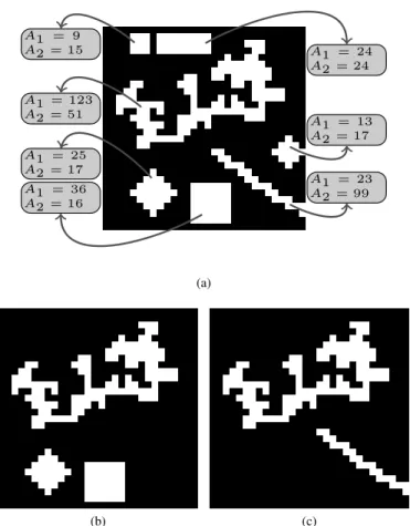
Figure 3 shows an example of attribute filtering on a binary image. Two attributes, A1 based on the size and A2 on
the shape of the regions, were computed on the connected components of the image (Fig. 3.a). The results of two thinning operators, one based on A1 and one onA2 (with an arbitrary
predicate), are shown in Figs. 3.b,c. It is worth noting that it is not possible to achieve the result in Fig. 3.c (i.e., removing all the foreground objects with a compact shape) with a single filtering based onA1. Vice versa, the removal of objects based
on their scale cannot be obtained consideringA2. Furthermore,
when considering connected operators based on SEs (such as opening and closing by reconstruction), the result in Fig. 3.b can be equivalently obtained with any SE that is not contained in the foreground objects of smaller scale (but contained in the three largest objects). However, as in Fig. 3.c, the result cannot be achieved straightforwardly with a single filtering based on a SE due to the different scale of the structures meant to be preserved.
There is an inclusion relations between the connected com-ponents in the image (obtained from the upper or lower sets) meaning that any two components are either nested or disjoint. Due to this, the set of connected components can be
repre-2We recall that for a generic transformation ψ on an image
f (and g), idempotence means ψ(ψ(f)) = ψ(f), increasingness
f≤g ⇔ ψ(f)≤ψ(g) ∀f, g and anti-extensivity (resp. extensivity) refers tof≥ψ(f)(resp.f≤ψ(f)). A1 = 9 A2 = 15 A1 = 123 A2 = 51 A1 = 25 A2 = 17 A1 = 24 A2 = 24 A1 = 13 A2 = 17 A1 = 23 A2 = 99 A1 = 36 A2 = 16 (a) (b) (c)
Fig. 3. Illustrative example for attribute filtering. (a) Binary image in which two different attributes were computed for each connected component of the image upper level set. Only connected components of the foreground are considered in this example. AttributeA1 is a scale dependent measure (i.e.,
the area in number of pixels for each region) andA2is a shape index invariant
to scale and rotation (i.e., the moment of inertia multiplied by a factor102
was considered as measure). (b) Result of a thinning with predicateA1>25.
(c) Result of a thinning with predicateA2>30.
sented by a tree being its nodes the components and the links between nodes the inclusion relations between components. The tree derived by the components in the upper (resp. lower) level set is called max-tree (resp. min-tree) [37].3 Another
representation of a gray-scale image as a hierarchy of regions is theinclusion tree. Here the set of connected components is
obtained by progressively “filling” regions internal to others (i.e., considered as “holes”) and the connections in the tree are determined by the considered region filling operator [39]. Such hierarchical representations of an image can be ef-fectively exploited for the computation of morphological AFs [37, 40]. Thinnings and thickenings will be obtained from a max- and a min-tree, respectively. The image transformation done by the filter on the image is equivalent to a pruning of the tree,i.e., the removal of single nodes or branches.
Different pruning strategies exist depending on whether the predicate evaluated by the AF is increasing or not [40]. The increasingness of a predicate leads to the removal of entire branches (i.e., a node with all its descendants till their leaves) from the tree. Conversely, for non increasing predicates, intermediate nodes in a branch can either fulfill
the predicate or not. For that case, different filtering rules have been defined in the literature [37, 41].
An example of max-tree is shown in Fig. 4. As one can see in Figure 4b, the image is composed by connected components of iso-intensity pixels. The max-tree maps each of all the connected components of the image to a node organized in a hierarchical tree structure (see Figure 4c). The root node of the tree represents the whole image at his lowest gray-level. The tree grows by connecting the nodes of the progressively nested connected components in the image until the leaves of the tree that correspond to the regional maxima in the image. 0 0 0 0 0 0 0 0 0 0 0 2 3 3 1 0 0 0 0 0 0 0 2 1 1 0 0 1 1 0 0 0 0 0 0 0 2 2 1 0 0 0 0 1 1 2 2 2 1 0 0 0 2 2 1 1 1 2 1 0 0 0 2 3 3 1 1 0 0 0 0 0 2 2 3 3 0 0 0 0 0 0 0 0 0 0 0 0 0 0 0 0 0 0 0 0 0 0 0 0 (a) C0 0 C00C00C00C00C00C00 C00 C00 C00 C0 0 C20C30C03C01C00C00 C00 C00 C00 C0 0 C00C20C01C01C00C00 C11 C11 C00 C0 0 C0 0 C0 0 C0 0C0 0C0 0C2 2 C2 2 C1 1 C0 0 C0 0 C0 0 C0 0 C1 1C1 1C2 2C2 2 C2 2 C1 1 C0 0 C0 0 C00C21C12C11C11C11 C22 C11 C00 C0 0 C00C21C13C13C11C11 C00 C00 C00 C0 0 C00C21C12C13C13C00 C00 C00 C00 C0 0 C00C00C00C00C00C00 C00 C00 C00 C0 0 C00C00C00C00C00C00 C00 C00 C00 (b) C0 0 C1 1 C2 2 C1 2 C1 3 C0 1 C0 2 C0 3 (c) Fig. 4. Example of Max-tree. (a) Gray-scale image with intensities ranging from 0 to 3; (b) Image in (a) with its connected components labeled; and (c) Max-tree of (a). This shows the relations between the nodes associated to the connected components in (b) [42].
B. Attribute Profile and its extension to vectorial images
Although this subsection should be considered self-sufficient for understanding the concept of AP, EAP and EMAP4, for more information regarding the aforementioned
concepts, please refer to [25, 42]. More useful references can be found throughout the paper.
APs are obtained by the outputs of a sequence of thinning and thickening transformations applied on a scalar image [25]. APs can be seen as a generalization of MPs since both opening and closing by reconstruction can be implemented as attribute filters [33]. The motivation for using attribute filters is to overcome the limitation of the conventional operators based on geodesic reconstruction in defining a decomposition of the image based on characteristics different from the scale [43]. In fact, MPs naturally perform a multiscale decomposition of an image, since structuring elements of a fixed shape and an increasing size are employed. However, trying to compute an MP based on the shape cannot be easily achieved since scale invariant characteristics are poorly modeled by SEs (it would require a very large set of SEs, since the analysis should be scale invariant and many different shapes of the SE should be considered). Instead, by using AFs, the image decomposition can be based on the scale (as for MP), shape, texture, etc. according to the type of attribute considered.
More formally, an AP is defined as in Eq. (1) [25]: with
Pλ:{Pλi} (i= 1, . . . , L) a set ofL ordered predicates (i.e.,
4The Matlab code for the use of AP, EAP and EMAP is available on request
by sending an email to the authors.
Pλi ⊆Pλk, i ≤ k). The sequence of criteria considered for
constructing the profile have to be ordered for guaranteeing the fulfillment of the absorption property, which might not be verified for non increasing predicates. Thus, the AP can be seen as a stack of thickening and thinning profiles. The thickening profile is considered in reversed order, such as the coarser image appears as first and the original image as last. The original imagef also appears in the profile since it can
be considered as the level zero of both the thickening and thinning profile (i.e., φPλ0(f) = γPλ0(f) = f, where Pλ
0
is a predicate which is fulfilled by all the components in the image, leading to no filtering). According to the attribute and criterion considered, different information can be extracted from the structures in the scene leading to different multilevel characterizations of the image. [25]. We refer the reader to [25] for further details. Fig. 8 shows an example for the general architecture of AP.
As mentioned previously, also in terms of computational burden, an AP is more advantageous than an equivalent MP, since the MP always demands two complete image transforma-tions: one performed by a closing and the other by an opening for each level of the profile. In contrast, for computing an AP it is necessary to build up one max-tree for the thinnings and one min-tree for the thickenings for the entire profile. The set of filtering is obtained by sequential pruning of the same trees with different values ofλ. This greatly reduces the burden of
the analysis with respect to MPs, since the most demanding phase of the filtering, which is the construction of a tree [44], is done only once.
We recall also that in [45], an inclusion tree was used for computing the AP instead of the min-tree and max-tree data representation, leading to a self-dual AP (SDAP). In that work, the application of self-dual connected operators led to an image simplification characterized by more homogeneous regions with respect to the results obtained by extensive or anti-extensive connected operators.
When dealing with vectorial images (f : E → T, with E⊆Z2andT ⊆Zn,n >1andf ={f
1, f2, . . . , fn}) such as multispectral and hyperspectral images (wherenis the number
of spectral bands), the application of morphological filters (here specifically APs) is not straightforward since there is no unique approach for extending them to vectorial images [46– 50, Chapter 11]. A possible way for applying the concept of the profile to vectorial images was proposed in [42, 51] and recalled in Sec. II.B. The proposed approach is based on the reduction of the dimensionality of the image values fromT to T0⊆Zm (m≤n) with a generic transformationΨ :T →T0
applied to an input image f (i.e., g = Ψ(f)) and then on
the application of the AP to each gi (i = 1, . . . , m) of the transformed image. This can be formalized as:
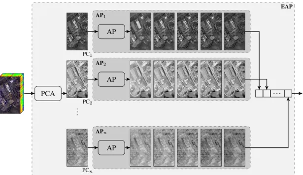
EAP(g) ={AP(g1), AP(g2), . . . , AP(gm)}. (2) Fig. 5 shows the general architecture of EAP.
It can be convenient to compute multiple EAPs considering different attributes in order to derive a more complete descrip-tor of an image. This is the underlyining idea of theExtended
EAP AP1 AP2 APn PC1 AP PC2 AP ... PCn AP PCA . . .
Fig. 5. General architecture of EAP.
EMAP EAP1 EAP2 EAPn
EAP
EAP
...
EAP
. . .
Fig. 6. General architecture of EMAP.
defined considering kdifferent attributes as: EM AP(g) = EAPA1(g), EAP 0 A2(g), . . . , EAP 0 Ak(g) , (3) where EAPAi is an EAP built with a set of predicates
evaluating the attribute Ai and EAP0 =EAP\{gi}i=1,...,m in order to avoid redundancy since the original components
{gi} are present in each EAP. Fig. 6 shows the general architecture of EMAP. The following attributes have been widely used in literature in order to produce EMAP:
1) Area of the region (related the size of the regions) 2) Standard deviation (as an index for showing the
homo-geneity of the regions)
3) Diagonal of the box bounding the regions
4) Moment of inertia (as an index for measuring the elongation of the regions).
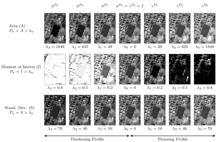
Fig. 7 shows an n example of different attribute profiles (Area, Moment of Inertia and Standard Deviation) with dif-ferent threshold values.
P3 3= 1849 Area (A) Pn=A > n P2 2= 625 P1 1= 49 P0= P0 =f 0= 0 P1 1= 49 P2 2= 625 P3 3= 1849 3= 0.8 Moment of Inertia (I)
Pn=I > n 2= 0.5 1= 0.2 0= 0 1= 0.2 2= 0.5 3= 0.8 3= 70 Stand. Dev. (S) Pn=S > n 2= 40 1= 10 0= 0 1= 10 2= 40 3= 70
Thickening Profile Thinning Profile
Fig. 7. An example of different attribute profiles (Area, Moment of Inertia and Standard Deviation) with different threshold values.
AP(f) = φPλL(f), φPλL−1(f), . . . , φPλ1(f) | {z } thickening profile , f, γPλ1(f), . . . , γPλL−1(f), γPλL(f) | {z } thinning profile , (1) AP Thickening Profile Thinning Profile T1 ... TL T1 ... TL . . . .
Fig. 8. Example of the general architecture of AP
IV. SPECTRAL-SPATIAL CLASSIFICATION BASED ON THE AP
Although this section should be considered self-sufficient for understanding the concept of spectral-spatial classification based on the AP, for more information regarding the aforemen-tioned concepts, please refer to [30, 52, 53]. More references can be found throughout the paper.
This section aims at reviewing the main steps composing the techniques based on APs for land cover classification. We will focus on the classification of hyperspectral images (thus considering EAPs/EMAPs) since most of those tech-niques were proposed for this imagery. It is underlined that this choice is done without loss of generality since all the classification architectures proposed for other types of data (e.g., panchromatic images in [54]) can be reconducted to
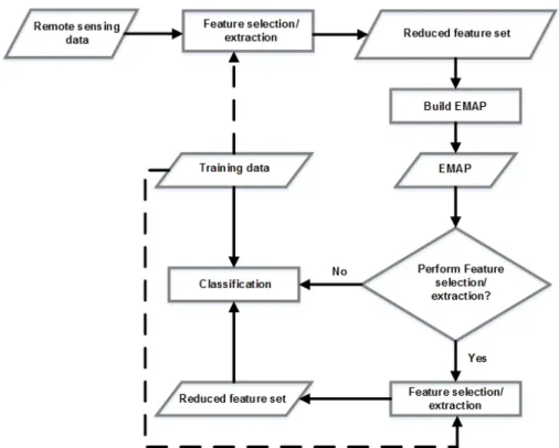
the general scheme presented in this section. A general work flow of the spectral-spatial classification with EMAP is shown in Fig. 9. First, feature extraction/selection is performed on remote sensing data and the resulting features are used as bases to build the EMAP. It should be noted that feature extraction/selection are mostly taken into account for hyper-spectral images in order to reduce the redundancy of the data and address the so-called curse of dimensionality. For other types of data, this step can be discarded. In [55], it
Fig. 9. The general work flow of spectral-spatial classification with EMAP. The dotted lines indicate the possibility of switching between supervised and unsupervised feature reduction. An optional feature reduction step can be used to reduce the dimensionality of EMAP before classification [52].
has been noted that a prior spectral decomposition based on kernel feature extraction before building the APs can lead to better classification results. The feature extraction/selection can either be supervised or unsupervised. A further feature extraction/selection operation applied to the EMAP can both reduce the effect of the Hughes phenomenon [20] and the redundancy in the profiles for classification. The classification is usually performed using non-linear classifiers due to the fact that the resulting EMAP is characterized by highly non-linear class distributions. In the following, the main components of the flowchart in Fig. 9 (Feature selection/extraction and classification) will be discussed in detail. Furthermore, at the end of this section, the automatic generation of EMAP for the accurate classification of remote sensing data will be discussed.
A. Feature extraction and feature selection
In the spectral domain, each spectral channel is considered as one dimension. By increasing the features in the spec-tral domain, theoretical and practical problems may arise. For instance, while keeping the number of training samples constant, the classification accuracy actually decreases when the number of features becomes large [20]. For the purpose of classification, these problems are related to the curse of dimensionality. In [56], it was shown that too many spectral bands can be undesirable from the standpoint of expected classification accuracy because the accuracy of the statistics estimation decreases (Hughes phenomenon). The aforemen-tioned issue demonstrates that there is an optimal number of bands for classification accuracy and more features do not necessarily lead to better results. Therefore, the use of
feature reduction techniques may lead to a better classification accuracy. The Hughes phenomenon highly influences on para-metric classifiers where the higher set of statistical estimations need to be estimated and their classification accuracies are dramatically downgraded by that effect. However, this issue has a less influence on non-parametric classifiers such as SVM [57] and Random Forest (RF) [58].
In order to fully exploit spatial information from different structures in the scene, different attributes with considerable range of threshold values should be considered. Nevertheless, considering many attributes with many threshold values can re-sult in hyperdimensional profiles and, thus, hyperdimensional feature vectors that can lead to Hughes phenomenon [20] (i.e., the curse of dimensionality) and a high redundancy since
filters with slightly different parameters may produce similar results. The issue of the high dimensionality of the profile can be addressed by considering feature reduction techniques. However, the selection of appropriate filter parameters is an essential step in order to guarantee a good tradeoff between the descriptive power of the profile and its redundancy [59]. In this case, FS and FE techniques have been gaining significant considerations in order to select the most effective features of the APs.
FS methods choose features from the original data set based on a criterion that is used to filter out unimportant or redundant features. FE can be explained as finding a set of vectors that represents an observation while reducing the dimensionality by transforming data to another domain. FE/FS can be split into two categories; unsupervised and supervised FE/FS where the former is used for the purpose of data representation and latter is considered for solving
the Hughes phenomena [20] and reducing the redundancy of data in order to improve classification accuracies by getting feedback from a set of available training samples. Although a reduction in dimensionality is of importance, the error rising from the reduction in dimension has to be without sacrificing the discriminative power of classifiers [32].
As can be seen from Fig. 9, FE/FS can be performed on the input data (in order to reduce the redundancy of the input data and select informative features as basis for producing APs), or on the obtained APs (in order to reduce the redundancy of obtained features by APs and increase the classification accuracies). It should be noted that FE/FS can as well be used for both steps in one classification framework.
1) FE: PCA, KPCA and ICA are the most commonly used
unsupervised FE which are used along with the concept of EMAP (eg., [30, 52, 60]). Moreover, DAFE, DBFE and NWFE are considered as the best known supervised FE which are taken into account along with the concept of EMAP (eg., [52]). It should be noted that the unsupervised FEs are mostly applied in order to extract informative features as the basis for producing APs. However, the supervised FEs can be performed on either the input data or the features obtained by APs.
The choice of the feature extraction method has also been found to greatly influence the classification results using EMAPs. In [52], various supervised and unsupervised feature extraction methods were compared when EMAPs were built using corresponding features and classified using RF and SVM classifiers. It has been concluded that kernel feature extraction methods (in this case kernel PCA) provides more consistent performance even if supervised feature extraction (e.g., DBFE,
NWFE, etc) produces more accurate maps when sufficient number of training samples are available. Furthermore, it has been noted in [55] that a prior feature extraction from multispectral data using kernel methods to build the EMAP produces significantly improved classification maps.
In order to classify informative features produced by su-pervised FE, the first features with cumulative eigenvalues above 99% are retained. In the case of DAFE and NWFE, the criterion is related to the size of the eigenvalues of the scatter matrices. In the case of decision boundary FE (DBFE), the criterion is related to the size of the eigenvalues of the decision boundary feature matrix (DBFM). For PCA, the first PCs with a cumulative variance of more than 99% are kept, since they contain almost all the variance in the data. However, different percentages can be used for different data.
Very recently in [61], it was proposed to compute a multiple profile composed of APs built on different base images obtained by linear, non-linear, manifold learning-based and multil-linear transformations of the original hyperspectral image. The individual APs computed on the extracted features (obtained by the different strategies) are either considered separately or jointly in a stacked vector. In order to deal with the high dimensionality of the profile, it was proposed to use a decision fusion approach or a sparse based classifier.
2) FS: In [59], an automatic method was introduced for
the classification of hyperspectral data which is based on the FS step. In order to reduce the number of features by only keeping those important, GAs based on a measure of
the relevance of the features were used. The main idea here is to construct a large profile from input hyperspectral data, called the EEMAP, that covers all the reasonable range of values for the filter parameters in order to provide a complete and detailed characterization of the spatial information of the scene. then, for reducing the number of features by only keeping the important ones, GAs based on a measure of the relevance of the features are taken into account.
In [62], a new FS technique was proposed which is based on the integration of GA and PSO. Then, the FS technique was applied on several features produced by EMAP for selecting the most informative features in order to detect road networks. In [63], a new feature selection technique is introduced, which is based on a new binary optimization method named BFODPSO. In that method, SVM is used as the fitness function and its corresponding classification overall accuracy is chosen as the fitness value in order to evaluate the efficiency of different group of features. In that paper, first, an AP feature bank is built consisting of different attributes with a wide range of threshold values. Then, BFODPSO based feature selection is performed on the feature bank. In this case, SVM is chosen as fitness function. The fitness of each particle is evaluated by the overall accuracy of SVM over the validation samples. After a few iterations, BFODPSO based feature selection approach finds the most informative features (resulted by EMAP) with respect to the overall accuracy of SVM over the validation samples.
In [64], a strategy for the selection of spatial features (among those APs were considered) relevant for classification was proposed. The relevance of the features is determined with respect to their capability in maximizing the SVM margin in the separation of classes. A research procedure based on the randomly generation of spatial filter banks and use of an active set criterion to rank the candidate features according to their benefits to margin maximization is proposed. In this way it is possible to explore the virtually infinite feature space (constituted by all the possible spatial features that could be computed) in order to retain the relevant ones for guaranteeing a final classification scheme which is compact (uses as few features as possible), discriminative (enhance class separation) and robust (works well in small sample situations).
B. Classification using different methods
As discussed above, APs have been successfully exploited as efficient tools for spectral-spatial classification of remote sensing data. APs are inherently characterized by a large dimensionality and high redundancy. This poses a great challenge for classification especially to counter the Hughes phenomenon [20]. Due to high non-linear characteristics of the class distributions in the APs, the classification should be performed using non-linear classifiers. A majority of the studies on classification of attribute profiles employed SVM [57] and RF [58] classifiers (e.g., [52, 59, 65]).
SVM is a well-known classifier which separates training samples of different classes by tracing maximum margin hyperplanes in the space where the samples are mapped [66]. SVMs were originally introduced to solve linear classification
problems. However, they were generalized for solving non-linear decision functions by using the so-called kernel trick [67]. A kernel-based SVM is used to project the pixel vectors into a higher dimensional space and estimate maximum margin hyperplanes in the new space, for improving linear separability of data [67]. The two main critical aspects of SVMs are the sensitivity to the choice of the kernel and the selection of the regularization parameters. The second issue can be classically overcome by considering cross-validation techniques using training data [68]. However, that can be computationally expensive [52]. The Gaussian RBF is the most widely used kernel in remote sensing [67]. The cross-validation explores an appropriate bandwidth parameter which provides the minimum error when the kernel-based SVM classifier is applied on the training data set. The main shortcomings of the cross validation are that 1) the bandwidth parameter needs to be discretized between a minimum and a maximum value, and the SVM classifier has to be trained and tested in a fivefold way for each of the discrete values of the bandwidth parameter. By increasing the number of discrete levels, the probability of finding the best parameter increases which leads to a higher computational time. On the contrary, by decreasing the number of levels, a sub-optimal bandwidth parameter might be selected [69]. 2) In most of data sets, the cross-validation procedure does not consider a convex error curve over the selected discrete bandwidth parameter values, which makes the selection of discrete bandwidth parameter values a difficult task [69]. In order to tackle the above mentioned problems, in [70], a gradient-based method was proposed to minimize the upper bound of the leave-one-out generalization error of SVM over the set of full-diagonal bandwidth parameters. In [69, 71], the upper bound was estimated based on the radius margin bound.
RF is an ensemble method for classification and regression. Ensemble classifiers get their name from the fact that several classifiers, i.e., an ensemble of classifiers, are trained and
their individual results are then combined to provide a final classification. For the purpose of classification of an object from an input vector, the input vector is run down each tree in the forest. Each tree provides a single vote for a particular class and the forest chooses the classification label having the most votes. Based on studies in [72], RF is not computationally intensive but demands a considerable amount of memory. RF can provide a good classification result in terms of accuracies and does not assume any underlying probability distribution for input data. Another advantage of RF classifier is that it is insensitive to noise in the training labels [72]. In addition, RF provides an unbiased estimate of the test set error as trees are added to the ensemble and finally it is less prone to overfit.
Apart from using SVM and RF classifiers, a composite kernel framework for spectral-spatial classification using APs has been recently investigated. In [73], a linearly weighted composite kernel framework with SVMs has been used for spectral-spatial classification using APs. A linearly weighted composite kernel is a weighted combination of different ker-nels computed using the available features [74]. For classifica-tion using APs, probabilistic SVMs were employed to classify the spectral information to obtain different rule images. The
kernels are computed using the obtained rule images and are combined using the weighting factor. The choice of the weighting factor can be given subjectively or estimated us-ing cross-validation. However, classification usus-ing composite kernels and SVMs require convex combination of kernels and a time consuming optimization process. To overcome these limitations, a generalized composite kernel framework for spectral-spatial classification using attribute profiles has been proposed in [73]. MLR ([75–77]) has been employed instead of SVM classifier and a set of generalized composite kernels which can be linearly combined without any constraint of convexity, were proposed.
Very recently, SRC techniques have been proposed for the classification of EMAPs [78]. SRC relies on the concept that an unknown sample can be represented as a linear combination of a set of labeled ones (i.e., the training set), called the dictionary. The representation of the samples is cast as an optimization problem in which the weights of each sample of the dictionary should be estimated with a constraint enforcing sparsity on the weights (i.e., limiting the contribution in the representation to only few samples). After representation, the sample is assigned to the class which shows the minimum reconstruction error when considering only the samples of the dictionary belonging to that class.
The importance of sparse-based classification methods has been further confirmed in [75] where a sparse-based MLR efficiently proved to handle effectively the very high di-mensionality of the AP-based features used as input to the classifier.
In [79], a new technique was introduced for the combined classification of a high spatial resolution color image and a lower spatial resolution hyperspectral image of the same scene. To this extent, 1) contextual information is extracted from the high spatial resolution color image by transforming the image into CIE-Lab space, In the new space, instead of working on the ’R’, ’G’, and ’B’ bands separately, APs are carried out on the ’L’ band, which corresponds to the Luminance, while the ’a’ and ’b’ bands (which contain the color information), are kept intact. Finally, the resulting images are transformed back into RGB space. 2) In parallel, the spectral information is extracted from the low spatial resolution hyperspectral data. 3) Finally, a composite decision fusion technique was investigated for combining the result of spectral and spatial information.
C. Automatic Scheme for EMAP
Although this subsection should be considered self-sufficient for understanding the concept of automatic EMAP, for more information regarding the aforementioned concepts, please refer to [30, 53, 59]. More references can be found throughout the paper.
In order to tackle the main difficulties of using the EMAP, which are 1) which attributes lead to a better discrimination for different classes, and 2) which threshold values should be considered in order to initialize each AP, automatic schemes of using EMAP has been investigated. While the APs can be constructed by using different attributes, in the automatic
scheme, generally the area and standard deviation attributes are only used, since these attributes can be adjusted in an automatic way and are well-related to the object hierarchy in the images [30, 53, 59].
The standard deviation is adjusted with respect to the mean of the individual features, since the standard deviation shows dispersion from the mean [65]. Therefore, λs is initialized in a way to cover a reasonable amount of deviation in the individual feature, and can be mathematically given by
λs(P Ci) =
µi
100{σmin, σmin+δs, σmin+ 2δs, ..., σmax},
(4) whereµi is the mean of thei-th feature andσmin,σmaxand
δs are inner bound, upper bound and step size for standard deviation attribute, respectively.
With regard to adjusting λa for the area attribute, the resolution of the image should be taken into account in order to construct an EAP [59]. The automatic scheme of the attribute area is given below:
λa(P Ci) =
1000
υ {amin, amin+δa, amin+ 2δa, ..., amax},
(5) where amin and amax are considered as inner and upper bounds, respectively, with a step size increaseδa andυshows the spatial resolution of the input data.
Here, ”automatic” means that the framework only needs to establish a range of parameter values in order to automatically obtain a classification result with a high accuracy for different data sets, instead of adjusting different thresholds with crisp values. More information regarding appropriate values for inner bound, upper bound and step sizes can be found in [30, 53, 59].
In [30], a spectral-spatial classification approach was in-troduced (please see the general idea of the model in Fig. 10a, which here this method is called MANUAL, since the threshold values for EMAP are adjusted manually). Then, in that paper, the automatic scheme of that method is devel-oped (please see the general idea of the model in Fig. 10b, which this method here is called AUTOMATIC, since the threshold values for EMAP are adjusted automatically with respect to (4) and (5)). Results reported in [30] for the both schemes (MANUAL and AUTOMATIC) are very close in terms of classification accuracies. The little difference obtained in the classification accuracies between the MANUAL and AUTOMATIC schemes can show that the use of only two attributes; area and standard deviation can model the spatial information on the used data sets considerably and other attributes (diagonal of the box bounding the region and the moment of inertia) cannot add significant improvement to classification accuracies although they carry information on the shape of regions. It is generally accepted that the use of different attributes will lead to the extraction of comple-mentary (and redundant) information from the scene leading to increased accuracies when used in classification (provided Hughes effect is efficiently solved by only keeping those features which are most informative). In summary, it can be inferred that the AUTOMATIC can provide classification maps comparable with the MANUAL in terms of both classification
accuracies and CPU processing time when only two attributes (area and standard deviation) are used instead of four (area, standard deviation, moment of inertia and diagonal of the box). However, the whole procedure in AUTOMATIC as the name indicates is automatic and there is no need for any parameters to be set.
In [65], the automatic generation of standard deviation attributes was introduced. As it was mentioned there, features commonly follow different statistics, and also, the individual classes have different statistics for different features. There-fore, different thresholds are needed to build the standard deviation profiles from different features. In this way, the thresholds for the standard deviation attribute are estimated based on the statistics of the classes of interest. The general idea behind that paper was that the standard deviation of the training samples of different classes of interest is related to the maximum standard deviation of the pixel values within individual segments of the corresponding classes of interest. The obtained results infer that the automatic method with only one attribute (standard deviation) along with supervised feature reduction can provide good results in terms of classification accuracies.
V. USE OF THEAPFOR DIFFERENT TYPES OF DATA AND APPLICATIONS
Although the concept of AP was introduced in order to extract spatial information from optical data (e.g.,
multispec-tral and hyperspecmultispec-tral data), this concept recently has been successfully exploited for characterizing spatial information of different types of data.
In [80, 81], the effectiveness of using EMAP for the classification of the joint use of optical and LiDAR data have been investigated. In [80], first the hyperspectral data were transformed by using PCA and first effective PCs were used as the base images for building EMAP. In parallel, different the intensity and the first return of LiDAR data were considered as inputs for building MAP. Then, all obtained profiles are concatenated into a stacked vector and classified by using either SVM or RF. Good classification accuracies obtained in that paper confirmed that APs can be effectively applied to LiDAR data, since they provide a simplification of the image reducing the noise caused by the irregular spatial sampling of the LiDAR pulse and the interpolation phase. To show the effectiveness of using AP, a comparison consider-ing texture features computed on GLCM have been taken into account. The results obtained by considering features extraction techniques along with the introduced technique have outperformed those achieved with GLCM features. Finally, in all the experiments, the application of EMAP on both optical and LiDAR data led to the best classification accuracies. Based on the results obtained in [81], the use of automatic EMAP can extract valuable information from LiDAR data by simultaneously filtering the unnecessary details and preserve the geometrical characteristics of the other regions.
In [54], feature extraction was carried out on polarimetric synthetic aperture radar images based on the decomposition of the covariance matrix and the corresponding features are
Input Data PCA EMAPEMAP Supervised FE Supervised FE RF Classification Map Spec AP (a) MAParea&STD(PC1) MAParea&STD(PC2) MAParea&STD(PCc) PCA 99% : : Supervised FE 99% Supervised FE 99% RF Stacked Vector (b)
Fig. 10. (a) The flowchart of the method introduced in [30] for the MANUAL classification of hyperspectral images using AP and feature extraction techniques; (b) The general idea of the AUTOMATIC scheme of the method introduced in [30]. The main idea here is that since PCA cannot consider the class specific information for producing EMAP, supervised FE is carried out on both the input data and features obtained by EMAP. The main difference of this figure with Fig. 9 is that in this method, features obtained by performing a supervised FE on both the EMAP and the input data are concatenated into a stacked vector and classified by RF. In this case, first, PCA is performed on the input data and first PCs with a cumulative variance of more than 99%are kept. Then, MAP including area and standard deviation attributes with respect to (4) and (5) are built for each PC. Furthermore, the MAP of different PCs are concatenated into a stacked vector. The output of this step provides spectral information. After that, the supervised FE is carried out on the stacked vector and first features corresponding to the top few eigenvalues which account for 99%of the total sum of the eigenvalues are kept. The output of this part provides the spatial information of the method. In parallel, the supervised FE is performed on the input data, and first features corresponding to the top few eigenvalues which account for 99%of the total sum of the eigenvalues are selected. The output of this step is considered as spectral information. As the last stage, the spectral and spatial information are concatenated in a stacked vector and the stacked vector is classified by RF [30].
used for building the APs. In the paper, the standard deviation is used as the attribute to build the EAP. The classification results show that there is an improvement when the EAP is used and a smoother classification result is obtained for visual examination of results.
The concept of the AP has been also used for different applications such as change detection. Although, the main objective of this paper is to investigate the usefulness of the AP for remote sensing image classification, other applications of the AP is briefly discussed below.
In [82], APs were employed for detecting changes occurred on the ground by analyzing two images acquired over the same areas before and after the occurred event. APs com-puted on each of the two images were compared in order to detect differences in the geometrical and morphological characteristics of the underlining structures present in the two images in corresponding zones. The reason motivating the use of APs for the detection of changes relies in the fact that if an abrupt change has occurred in the scene (e.g., a
man-made change or a natural disaster) it will be likely that the spatial characteristics of the affected areas will have changed too. Thus, by detecting differences in the behaviors of the APs in corresponding positions in the image can be useful for spotting a modification in the spatial arrangement of the pixels values between the two images. The change detection technique was based on three main steps: 1) Application of the APs to each image; 2) Region extraction and reliable level selection by analyzing the DAPs; 3) Comparison of the APs and generation of the change-detection map.
VI. DISCUSSION
As can be seen from Fig. 9, the use of appropriate FE/FS techniques and efficient classifiers can significantly influence on the obtained classification accuracies and the quality of the classification map. Therefore, in this section, leveraging the outcomes presented in the literature, the capability of different FE/FS techniques as well as different classifiers will be investigated.
A. The influence of different FE/FS along with AP on the classification accuracies
Although this subsection should be considered self-sufficient for understanding the influence of different FE/FS along with AP on the classification accuracies, for more information regarding the aforementioned concepts, please refer to [30, 52, 53]. More references can be found throughout the paper.
1) When only spectral information derived by NWFE, DAFE and DBFE is used, the result of the classification is almost the same. However, when the corresponding EMAP based on DAFE, DBFE, NWFE is made, the accuracies are quite different which shows that the classification with EMAPs do not necessarily follow the trend of classification with spectral information only [52, 53].
2) When the number of training samples is limited, a super-vised FE leads to less accurate results in terms of classi-fication accuracy compared to unsupervised techniques. In [83], it was mentioned that the combination of KPCA and EMAPs can be a simple even powerful strategy
to perform spectral-spatial classification of data sets with limited spectral resolution (RGB and multispectral images). With reference to [52], in general, EMAP based on KPCA can be found more consistent even though it sometimes produces slightly inferior accuracies in comparison with the supervised feature extraction techniques. However, it is difficult to anticipate which supervised feature extraction technique is appropriate for a problem at hand and the performance of that is highly dependent on the number of available training samples. 3) In a case when the number of training samples is sufficient, according to the experiments shown in [52], DBFE seems to be able to provide better results in terms of classification accuracies than DAFE and NWFE in order to produce EMAP.
4) Based on the results reported in [30], the CPU pro-cessing time for the both schemes (MANUAL and AUTOMATIC) is almost the same. For AUTOMATIC, there is no need to adjust the initial parameters for the attribute profiles which is considered as the main shortcoming of the usage of AP.
5) The results obtained in [84] show that the selection strategy is able to retrieve for each class its optimal discriminant features. Remarkably, that technique effec-tively handled different types of spatial features (e.g.,
textural features and APs). In addition, it was shown that the models trained on the features discovered reached at worst the same performances as considering predefined filter banks (i.e., manual selection of the filter parameters requiring prior knowledge).
6) In [53], a spectral-spatial classification framework was developed which is specifically related to the use of para-metric supervised feature extraction techniques (DAFE and DBFE) and EMAP. Results show that when different parametric supervised feature extraction techniques is used for the first and second steps (e.g., DBFE is applied
on the input data and DAFE is carried out on the features extracted by EMAP or vice versa) and the first features corresponding to the top few eigenvalues of the both steps are concatenated into a stacked vector, the result of the classification is good and RF can classify the stacked vector of features accurately.
B. A comparison of different classifiers used with EMAP
Although this subsection should be considered self-sufficient for understanding the influence of different classi-fiers on the classification accuracies for the features produced by AP, for more information regarding the aforementioned concept, please refer to [30, 52, 53]. More references can be found throughout the paper.
Below, the main points regarding the applicability of SVM and RF are listed:
1) While both SVM and RF classification methods are shown to be effective classifiers for non-linear clas-sification problems, SVM requires a computationally demanding parameter tuning process (cross-validation) in order to tune hyperplane parameters and consequently
achieve optimal results, whereas RF does not require such tuning process. In this sense, RF is much faster than SVM and for volumetric data using RF instead of SVM is favorable.
2) The effect of the Hughes phenomenon is more evident when the number of dimensionality is high and the data is classified by SVM. Better accuracy values are achieved with SVM only after a further feature reduction [52].
3) RF is more stable when limited training samples are available. Even when a sufficient number of training samples are available, the SVM classifier required fur-ther feature reduction of the profile to achieve acceptable classification accuracy [65].
4) Based on the results reported in [52, 53, 65], RF provides higher classification accuracies compared to SVM when it is directly performed on EMAP, but SVM performs better in terms of classification accuracies when a further feature extraction is performed on EMAP. This shows the capability of RF in order to handle a higher dimen-sional space as an input to the classifier. On the contrary, the second feature extraction on EMAP downgrades the classification accuracies of the RF classifier. The reason of that might be the RF classifier is based on a collection of a weak classifiers, which can statistically take advantage from a large set of redundant features. In contrast, the SVM classifier seems to be more effective in designing discriminant function when a subset of non-redundant features defines a highly non-linear problem. 5) The experiments in [75] showed significant improvement in classification accuracies when the generalized com-posite kernel framework is used when compared to the regular composite kernel framework.
6) From the result obtained with SRC coupled with EMAPs [73], it can be stated that SRC outperforms other clas-sifiers such as SVM and SVM with composite kernels especially when the number of training samples is small.
C. A comparison of different classification maps obtained by EMAP
This subsection is based on the comparison of different classification maps obtained by EMAP and different FEs. In order to precisely evaluate different classification maps, two different scenarios are taken into account. The first scenario is devoted to a situation when the number of training samples is not sufficient. For this purpose, a frequently used, Indian
Pines data set is used. For more information related to the
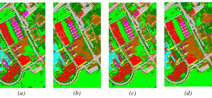
number of training and test samples, please see [52]. The second scenario is devoted to a situation when the number of training samples is sufficient. For this purpose, a frequently used,Pavia Universitydata set is used. For more information
related to the number of training and test samples, please see [30].
Scenario (1) When the number of training samples is
limited:
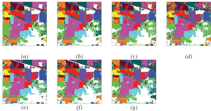
By visually comparing the classification maps shown in Figs. 11 and 12, the following points can be obtained:
(a)
(b)
(c)
(d)
(e)
(f)
(g)
Fig. 11. Classification maps for Indian Pines data with RF classifier (with 200 trees) using EMAPs of (a) PCA (OA=92.83%), (b) KPCA (OA=94.76%), (c) DAFE (OA=84.33%), (d) DBFE (OA=87.23%) and (e) NWFE (OA=95.06%), and feature reduction applied on EMAP using (f) NW-NW (OA=91.03%) and (g) KP-NW (OA=90.36%) [52]
(a)
(b)
(c)
(d)
(e)
(f)
(g)
Fig. 12. Classification maps for Indian Pines data with SVM (with 5-fold cross validation and RBF kernel) classifier using EMAPs of (a) PCA (OA=86.53%), (b) KPCA (OA=90.20%), (c) DAFE (OA=70.69%), (d) DBFE (OA=78.39%) and (e) NWFE (OA=81.85%), and feature reduction applied on EMAP using (f) NW-NW (OA=94.17%) and (g) KP-NW (OA=93.75%) [52]

![Fig. 10. (a) The flowchart of the method introduced in [30] for the MANUAL classification of hyperspectral images using AP and feature extraction techniques;](https://thumb-us.123doks.com/thumbv2/123dok_us/9959467.2488435/13.918.90.836.108.376/flowchart-introduced-manual-classification-hyperspectral-feature-extraction-techniques.webp)