Memory and persistence in models of volatility in financial time series

Memory and persistence in models of volatility

in …nancial time series

Submitted by Xiaoyu Li

to the University of Exeter as a thesis for the degree of

Doctor of Philosophy in Economics

June 2016

This thesis is available for Library use on the understanding that it is copyright material and that no quotation from the thesis may be published without proper acknowledgement.

I certify that all material in this thesis which is not my own work has been identi…ed and that no material has previously been submitted and approved for the award of a degree by this or any other University.

ACKNOWLEDGEMENTS

I would like to express my sincere gratitude to my …rst supervisor, Professor James Davidson, for his patient guidance, continuous encouragement and support of my PhD research. He has been the best advisor for my PhD studies in my mind. I would also like to thank my second supervisor, Dr Andreea Halunga, for her useful comments and suggestions.

I gratefully acknowledge the funding from the ESRC.

I am grateful to the sta¤ of the Business School at the University of Exeter, especially to Kate Gannon and Helen Bell, for their support and help throughout my PhD studies. I also thank my colleagues and friends for all their encouragement and support.

I also thank the participants at the following conferences, who made comments on my research: University of Exeter Economics Seminar 2011-2016; 7th and 9th International Conference on Computational and Financial Econometrics, London, 2013 and 2015; 11th International Vilnius Conference on Probability Theory and Mathematical Statistics, 2014.

Finally, I would like to thank my whole family for their love and support, especially my parents and my husband, Yuchen Wei.

ABSTRACT

This thesis …rst investigates the moment and memory properties of exponential-type conditional heteroscedasticity models. This primarily includes exponential generalised autoregressive conditional heteroscedastic (EGARCH) models, the frac-tionally integrated EGARCH model of Bollerslev and Mikkelsen (1996) (GARCH(BM)), the hyperbolic EGARCH (HYEGARCH) model and the FIE-GARCH(DL) model, as presented in Chapter 2. The moment conditions of these models are derived from previous literature, and the memory properties are mea-sured by using the near-epoch dependence (NED) functions of an independent process approach. The existence of moments supports the limited memory proper-ties of these models. This study shows that exponential autoregressive conditional heteroscedastic (EARCH)(₁) processes may exhibit geometric memory, hyperbolic memory or long memory. The EGARCH is a case of a geometric memory process. The FIEGARCH(BM) and HY/FIEGARCH(DL) processes can exhibit hyperbolic memory or long memory, depending on the sign of the memory parameter. The study also derives the functional central limit theorem (FCLT) or fractional FCLT for the relevant processes in these exponential-type conditional heteroscedasticity models. Finally, the results of the simulation show that the HYEGARCH model has a hyperbolic memory and that the FIEGARCH(DL) model can capture long memory in absolute return series.

Next, the study investigates the asymptotic properties of the quasi-maximum likelihood estimator (QMLE) in autoregressive moving average (ARMA) models with EGARCH or HY/FIEGARCH(DL) errors in Chapter 3. This part of the study aims to investigate the asymptotic theory of the ARMA(1;1)-EGARCH(1;1) models and that of the pure HY/FIEGARCH(DL) models. First, the literature

on the asymptotic properties of the ARMA-GARCH and EGARCH processes is reviewed. The conditions for the consistency and asymptotic normality of the QMLE of the ARMA-EGARCH models are then demonstrated. This analysis also provides an investigation of that of the QMLE in the HY/FIEGARCH(DL) processes. A Monte Carlo simulation is used to study the properties of the QMLE in the pure HY/FIEGARCH(DL) processes.

Lastly, in a study co-authored with Professor James Davidson, we derive a simple su¢ cient condition for strict stationarity in the ARCH(₁) class of processes with conditional heteroscedasticity. The concept of persistence in these processes is explored, and is the subject of a set of simulations showing how persistence depends on both the pattern of the lag coe¢ cients of the ARCH model and the distribution of the driving shocks. The results are used to argue that an alternative to the usual method of ARCH/GARCH volatility forecasting should be considered.

TABLE OF CONTENTS Acknowledgements . . . 2 List of Tables . . . 11 List of Figures . . . 12 1 Introduction 13 1.1 Basic concepts . . . 20

2 Moment and memory properties of the exponential-type

condi-tional heteroscedasticity models 24

2.1 Introduction . . . 24 2.2 Literature review . . . 28 2.2.1 Relevant volatility models . . . 28 2.2.2 Literature on the moment property of conditional

heteroscedas-ticity models . . . 30 2.2.3 The memory property of conditional heteroscedasticity models 32 2.2.4 The FCLT and fractional FCLT of conditional

heteroscedas-ticity models . . . 33 2.3 Exponential-type conditional heteroscedasticity models . . . 35

2.4 Moment properties of the exponential-type conditional

heteroscedas-ticity models . . . 39

2.5 Memory properties of the exponential-type conditional heteroscedas-ticity models . . . 43

2.5.1 Memory properties of the EGARCH-type models . . . 43

2.5.2 The HYEGARCH and FIEGARCH(DL) models . . . 48

2.6 FCLT and fractional FCLT for the EGARCH-type models . . . 50

2.6.1 The FCLT for the EGARCH(p; q) process . . . 52

2.6.2 Investigation of the FCLT and fractional FCLT for the FIE-GARCH(BM) process . . . 54

2.6.3 Investigation of the FCLT and fractional FCLT for the HYE-GARCH and FIEHYE-GARCH(DL) processes . . . 55

2.7 Simulation for the memory properties of HYEGARCH and FIE-GARCH(DL) processes . . . 57

2.7.1 Data generating process . . . 57

2.7.2 Estimation procedure and simulation results . . . 58

2.8 Conclusion . . . 59

2.9 Appendix A . . . 61

2.9.2 Proof of Theorem 2.5.3 . . . 65

2.9.3 Proof of Theorem 2.6.4 . . . 66

2.9.4 Proof of Theorem 2.6.5 . . . 67

2.9.5 Proof of Theorem 2.6.6 . . . 68

3 Asymptotic theory of the QMLE in ARMA models with EGARCH and HY/FIEGARCH errors 71 3.1 Introduction . . . 71

3.2 Literature review . . . 73

3.2.1 Stationarity and ergodicity properties of the relevant volatil-ity models . . . 74

3.2.2 Asymptotic theory of the QMLE in ARCH/GARCH models 75 3.2.3 Asymptotic theory of the QMLE in ARMA-type models with GARCH-type errors . . . 76

3.2.4 Asymptotic theory in the EGARCH-type models . . . 77

3.2.5 Finite sample properties of the EGARCH-type models . . . 80

3.3 The models and the QMLE . . . 81

3.3.1 The ARMA(1,1)-EGARCH(1,1) model . . . 81

3.3.2 The HY/FIEGARCH models . . . 83

3.4 The invertibility of the EGARCH-type processes . . . 87

3.4.1 Invertibility of the EGARCH(p; q) process . . . 87

3.4.2 Invertibility of the ARMA-EGARCH process . . . 95

3.4.3 Invertibility of the HYEGARCH process . . . 98

3.4.4 The invertibility of the derivatives of the ARMA-EGARCH process . . . 101

3.5 Asymptotic theory of the QMLE in ARMA(1,1) with an EGARCH(1,1) error . . . 104

3.5.1 Consistency of the QMLE in ARMA(1,1)-EGARCH(1,1) process105 3.5.2 Asymptotic normality of the QMLE in ARMA(1,1) with an EGARCH(1,1) error . . . 106

3.6 The asymptotic theory of the QMLE in HY/FIEGARCH processes 110 3.6.1 Asymptotic theory of the QMLE in the HYEGARCH process 111 3.6.2 Investigation of the asymptotic theory of the QMLE in the FIEGARCH process . . . 118

3.6.3 Simulations for the HY/FIEGARCH models . . . 120

3.7 Conclusion . . . 120

3.8 Appendix B . . . 125

3.8.2 Proof of Lemma 3.5.1 . . . 129 3.8.3 Proof of Lemma 3.5.2 . . . 130 3.8.4 Proof of Lemma 3.5.3 . . . 133 3.8.5 Proof of Theorem 3.5.2 . . . 135 3.8.6 Proof of Lemma 3.5.4 . . . 136 3.8.7 Proof of Lemma 3.5.5 . . . 141 3.8.8 Proof of Lemma 3.5.6 . . . 145 3.8.9 Proof of Lemma 3.6.1 . . . 151 3.8.10 Proof of Lemma 3.6.2 . . . 152 3.8.11 Proof of Lemma 3.6.3 . . . 153 3.8.12 Proof of Lemma 3.6.4 . . . 156 3.8.13 Proof of Lemma 3.6.5 . . . 157 3.8.14 Proof of Lemma 3.6.6 . . . 159 3.8.15 Proof of Theorem 3.6.2 . . . 160 3.8.16 Proof of Lemma 3.6.7 . . . 161 3.8.17 Proof of Lemma 3.6.8 . . . 163

4 Strict stationarity, persistence and volatility forecasting in ARCH(₁)

4.1 Introduction . . . 166

4.2 Literature review . . . 170

4.2.1 The stationarity of the ARCH-type models . . . 170

4.2.2 Persistence in the ARCH(₁) process . . . 176

4.3 Stationarity and persistence in ARCH(₁)-class processes . . . 178

4.4 Measuring the persistence of stationary time series . . . 186

4.4.1 JT statistics . . . 187

4.4.2 GPH estimator and that for the normalised ranks series . . . 189

4.4.3 Persistence measures . . . 190

4.5 Some simulation experiments . . . 191

4.5.1 Date generation process . . . 191

4.5.2 Measurement approach and simulation results . . . 193

4.6 Implications for volatility forecasting . . . 197

4.7 Conclusion . . . 203

4.8 Appendix C . . . 205

4.8.1 Proof of Proposition 4.3.1 . . . 205

4.8.2 Proof of Proposition 4.3.2 . . . 207

LIST OF TABLES

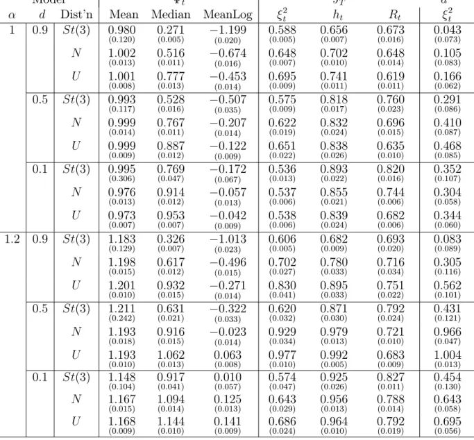
2.1 Simulation results for the HYEGARCH and FIEGARCH(DL) processes. 60 3.1 Simulation results for the QMLE in the HYEGARCH(0; d;0) process.121 3.2 Simulation results for the QMLE in the FIEGARCH(0; d;0) process.121 4.1 Persistence measures in a fractional linear time series, . . . 191 4.2 Series properties and persistence measures for the covariance

sta-tionary GARCH(1;1) model. . . 195 4.3 Series properties and persistence measures for the nonstationary

GARCH(1;1) model. . . 196 4.4 Series properties and persistence measures for the covariance

sta-tionary HY/FIGARCH model. . . 197 4.5 Series properties and persistence measures for the nonstationary

HY/FIGARCH model. . . 198 4.6 2MAV 2-step forecast error in GARCH(1;1), against M. . . 203 4.7 MAV 2-step forecast error in HY/FIGARCH, against M. . . 204

LIST OF FIGURES

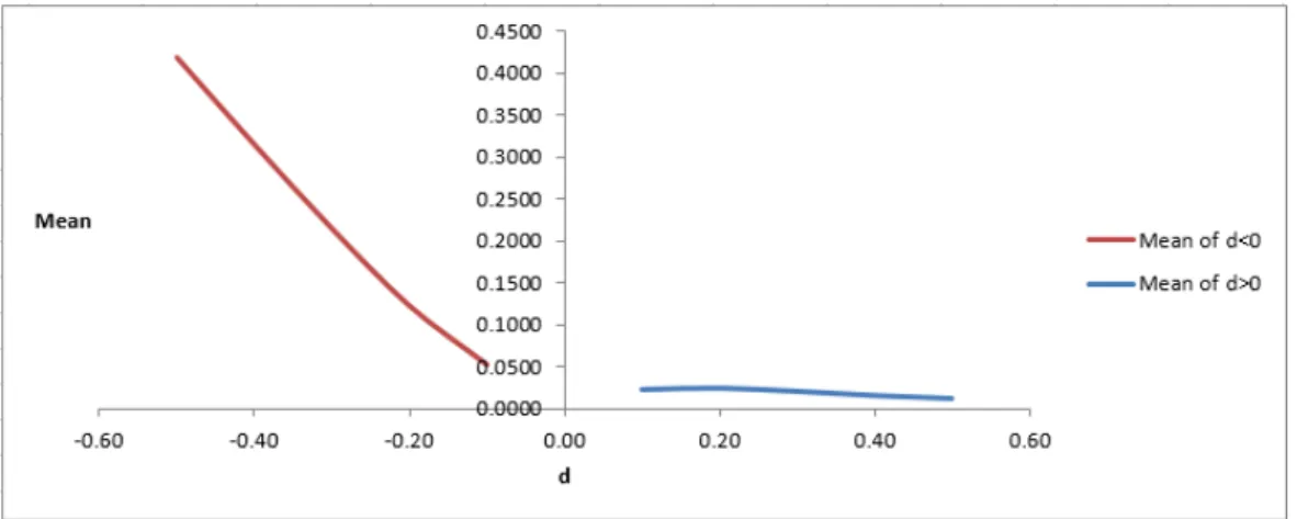
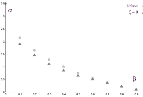
2.1 Simulation plots of the pure HYEGARCH and FIEGARCH(DL) models. Note: This …gure provides a corresponding plot of the simulation results presented in Table 2.1. The estimated memory parameters in the HYEGARCH and FIEGARCH(DL) models are indicated by a blue line and a red line, respectively. It is clear to see that the estimated memory parameters in the HYEGARCH model are very close to zero but, in the FIEGARCH(DL) model, the estimated memory parameters increase consistently with the absolute value ofd. . . 60 4.1 Gaussian GARCH(1;1) model: ( ; ) pairs where = 0 and the

stationarity boundary points of Nelson (1990). Note: this …gure provides some numerical experiments with Gaussian shocks show-ing -values at which 0 for = 0;0:1;0:2; : : : ;0:9. The mean is estimated in each case as the average of20;000 values of ln( t).

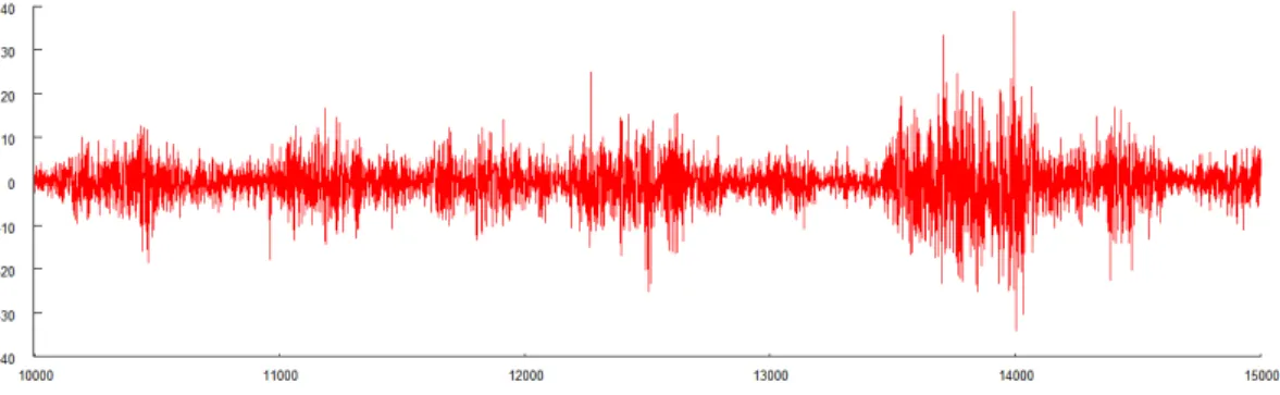
The actual stationarity boundary points from Nelson (1990) are also shown for comparison. . . 181 4.2 Simulation of IGARCH(1,1) with Student(3) shocks. Note: This

…gure provides the simulation results for samples of size 5000, with 10,000 pre-sample steps, for the IGARCH(1,1) model with ! = 1,

= 0:9 and Student(3) shocks. It shows the persistence proper-ties of the IGARCH(1,1) process with Student(3) shocks. More interpretations of this …gure are shown in Section 4.3. . . 184 4.3 Simulation of IGARCH(1,1) with Gaussian shocks. This …gure

fol-lows same simulation procedure to …gure 4.2, except it considers the IGARCH(1,1) process with Gaussian shocks. This …gure shows the persistence properties of the IGARCH(1,1) process with Gaussian shocks. More interpretations of this …gure are shown in Section 4.3. 184 4.4 Simulation of IGARCH(1,1) with uniformly distributed shocks. Note:

This …gure follows same simulation procedure to …gure 4.2, ex-cept it considers the IGARCH(1,1) process with uniformly distrib-uted shocks. This …gure shows the persistence properties of the IGARCH(1,1) process with uniformly distributed shocks. More in-terpretations about this …gure are shown in Section 4.3. . . 184

CHAPTER 1 INTRODUCTION

Volatility modelling and forecasting play an important role in option pricing, dynamic capital theory and asset pricing theory. Over the last few decades, many methods of volatility modelling have been introduced. Among these methods, En-gle (1982) …rst introduced the autoregressive conditional heteroscedastic (ARCH) model to investigate the volatility of UK in‡ation. The expression of the ARCH(p) model is shown in Equations (1.1) to (1.3):

t= p htzt; (1.1) ht =!+ p X j=1 j 2t j; (1.2) ht=E[ 2tjFt 1]; (1.3)

where_{f tg}is a real-valued discrete time stochastic process, which can also be inter-preted as a return series; process_fztgis an independent and identically distributed

(i.i.d.) stochastic variable with a mean of zero and a variance of one, such that zt i:i:d:(0;1), which can be interpreted as an innovation or shock; and

p

ht has

a positive value with a probability of one, such that pht>0, and it can be

inter-preted as the volatility of the return series. The series of t is independent because

the underlying series zt is an i.i.d. and is independent of

p

ht. In Equations (1.2)

and (1.3), ht is the conditional variance of t, and the Ft 1-measurable function,

where_Ft 1 is the -algebra generated byfzt 1;zt 2; :::g;indicating the information up to and including timet 1. The well-de…ned ARCH(p) processes require that ! >0, and j 0 (j = 1;2; :::; p). Since Engle’s study was published, the ARCH

processes have been widely used for modelling …nancial time series because they can capture the stylised facts of …nancial data, such as volatility clustering and

leptokurtic characteristics. Bollerslev (1986) proposed the generalised ARCH(p; q)

model, which is de…ned in Equations (1.1) and (1.4) ht = !+ q X i=1 i 2t i+ p X j=1 jht j (1.4) = !+ (L) 2_t + (L)ht;

where all parameters are non-negative, L denotes the lag operator, (i.e. Lk_z t =

zt k), and (L) = 1L+ 2L2+ + qLq and (L) = 1L+ 2L2+ + pLp are

polynomials in the lag operator. Equation (1.4) is the benchmark GARCH(1;1) model when p=q = 1.

Although the GARCH (p; q) process represents signi…cant progress and is very popular, it has some drawbacks. For example, it is unable to capture some of the characteristics of the volatility, such as asymmetric and long memory (a descrip-tive de…nition is provided in Section 1.1). To overcome these drawbacks, several conditional heteroscedasticity models have been proposed. In order to capture the asymmetric properties of the volatility, the exponential GARCH (EGARCH), the Glosten–Jagannathan–Runkle GARCH (GJR-GARCH) and threshold GARCH (TGARCH) models were introduced by Nelson (1991), Glosten et al. (1993) and Zakoïan (1994) respectively. To capture the high persistence properties of …nancial data, several conditional mean models, such as I(1) and I(d), have been extended to conditional variance models based on similar ideas. For instance, Engle and Boller-slev (1986) proposed the integrated GARCH (IGARCH) model, and Baillie et al. (1996) introduced the fractionally integrated GARCH (FIGARCH) model. How-ever, the IGARCH model exhibits short memory or geometric memory, see Ding and Granger (1996) and Davidson (2004), and the stationary FIGARCH fails to capture the long memory property of volatility, see e.g. Giraitis et al. (2009). In addition, Robinson (1991) introduced the ARCH(₁) to model long-run

depen-dence in volatility, but the squares 2_t from the stationary ARCH(₁) process does not allow the existence of long memory in volatility. Nevertheless, the mem-ory properties of the nonstationary ARCH(₁) process, including the IGARCH and FIGARCH models, have not been fully explored. Chapter 4 discusses the persistence in the IGARCH, FIGARCH and ARCH(₁) processes further.

A few models have also attempted to capture both the asymmetric and high per-sistence properties of volatility. For instance, the linear ARCH (LARCH) process and the fractionally integrated EGARCH (henceforth FIEGARCH(BM)) model were introduced by Robinson (1991) and Bollerslev and Mikkelsen (1996), respec-tively. In addition, in order to distinguish between the di¤erent memory properties of the EGARCH-type models, a general hyperbolic/fractional integrated EGARCH (henceforth HY/FIEGARCH (DL)) is proposed in Chapter 2. A stochastic volatil-ity class model was also introduced by Breidt et al. (1998) and Harvey÷(2002), namely the long memory stochastic volatility (LMSV) model. Ruiz and Veiga (2008) developed the theoretical property of the asymmetric LMSV (A-LMSV) model.

Research on the statistical properties of these conditional heteroscedasticity models has attracted a substantial amount of attention, since these models are widely used in practice. Among these models, the theoretical properties of the ARCH and GARCH models have been extensively explored. The memory prop-erty and the asymptotic theory of the estimator of the parametric LARCH process have been well developed by Giraitis et al. (2000b), Giraitis et al. (2004), Schützner (2009), and Beran and Schützner (2009), although some of the theoretical proper-ties remain unresolved. The statistical properproper-ties of the LMSV models are worthy of further academic consideration, but these are more complex and are therefore

not included in this thesis. In addition, mystery continues to surround the theo-retical properties of EGARCH-type models, even these have been investigated in a few recent studies, such as Surgailis and Viano (2002), Ruiz and Veiga (2008), and Lopes and Prass (2014).

The second and third chapters of this thesis investigate the theoretical proper-ties of EGARCH-type models. More speci…cally, Chapter 2 considers the moment and memory properties of EGARCH-type models, and near-epoch dependence (NED) is applied to measure the memory property and establish the functional central limit theorem (FCLT) and fractional FCLT of the relevant processes. The main reasons for undertaking this study are as follows. Firstly, this idea was in-spired by Davidson’s (2004) study, which investigated the moment and memory properties of linear conditional heteroscedasticity models. These properties are the two main statistical features of such models. Research on the moment properties of conditional variance models is useful for measuring how large the e¤ects of shocks to volatility can be, and the existence of moments is a necessary condition for determining the memory properties of conditional heteroscedasticity models, see e.g. He and Teräsvirta (1999a) and Davidson (2004). The memory property shows how long the e¤ect of shocks on conditional variance can persist, see e.g. Giraitis et al. (2000a), Davidson (2004) and Giraitis et al. (2009). Therefore, research on these properties is signi…cant for volatility estimation and forecasting.

Secondly, motivated by Davidson (2004), in Chapter 2, the NED concept is applied to measure the memory property of EGARCH-type models. A descriptive de…nition of the NED is provided in Section 1.1. The main reason for applying the NED approach is that this method may be easier for parameter estimation and inference in relevant models, especially for nonlinear and long memory conditional

heteroscedasticity models. Davidson (2004) introduced geometric and hyperbolic memory when applying the NED approach to measure the persistence of linear con-ditional heteroscedasticity models including GARCH, IGARCH, FIGARCH and HYGARCH. The theoretical and empirical results show that ARCH(₁) processes may exhibit hyperbolic memory or geometric memory, the FIGARCH process has hyperbolic memory, and both the standard GARCH and IGARCH processes have geometric memory. However, the models in Davidson (2004) did not include the EGARCH-type models. This is discussed further in Chapter 2.

Thirdly, the FCLT and fractional FCLT are vital for statistical inference of …nancial time series. The descriptive de…nitions of the FCLT and fractional FCLT are provided in Section 1.1. The concept of NED is applied for the FCLT, as was proposed by McLeish (1975). It satis…es the conditions for the law of large numbers (LLN), the central limit theorem (CLT), FCLT and fractional FCLT, and its restrictions can easily be veri…ed. (see e.g. Davidson, 1992, 1993, 1994; De Jong and Davidson, 2000; Davidson and De Jong, 2000). Thus the …rst aim of Chapter 2 is to investigate the existence of the …nite order moment of the relevant processes and, following a similar procedure to Davidson (2004), to study the NED properties of the EGARCH-type models, and then to measure the memory properties of these models by applying the concept of NED on an independent process. The second aim is to construct the FCLT and fractional FCLT for the relevant EGARCH-type models.

Chapter 2 makes three main contributions. Firstly, it shows that EARCH(₁) processes can have hyperbolic memory, geometric memory and long memory, as the EGARCH is a geometric memory process, the FIEGARCH(BM) with a nega-tive memory parameter has a hyperbolic memory, and the FIEGARCH(BM) with

a positive parameter can capture long memory in volatility. Secondly, this study provides a general HY/FIEGARCH(DL) process, that the HYEGARCH process has hyperbolic memory and the FIEGARCH(DL) process exhibits long memory. Thirdly, it establishes the FCLT for the EGARCH and the fractional FCLT for the partial sum of the _flnht !g processes in the FIEGARCH(BM) and

FIE-GARCH(DL) models.

Chapter 3 focuses on establishing an asymptotic theory of the quasi-maximum-likelihood estimators (QMLE) in the ARMA model with EGARCH-type errors. The QMLE is a popular estimation method for conditional heteroscedasticity mod-els. The ARMA model with EGARCH-type innovations has been widely used in empirical analyses of the …nancial time series. The asymptotic properties of the QMLE in the ARMA, GARCH and ARMA-GARCH processes have already been examined in detail (Weiss, 1986; Lee and Hansen, 1994; Ling and McAleer, 2003; Francq and Zakoïan, 2004; Straumann, 2005). However, only a few recent studies have focused on the asymptotic theory of the EGARCH process. For example, Straumann (2005) and Straumann and Mikosch (2006) proved the consistency of the QMLE in EGARCH (1;1) and asymptotic normality for EGARCH(1,0) under strong conditions. Wintenberger (2013) established the strong consistency of the QMLE, and the consistency and asymptotic normality (CAN) of the stable QMLE in the EGARCH(1;1) process under conditions that are di¢ cult to verify. Mar-tinet and McAleer (2015) investigated the asymptotic theory of the EGARCH(p; q) model by deriving it from a stochastic process, which made it easier to verify the invertibility conditions. However, some open questions in this area are yet to be answered, especially regarding the asymptotic properties of the QMLE for the ARMA-EGARCH and HY/FIEGARCH(DL) models. Therefore, it is vital to in-vestigate the asymptotic properties of the estimators in the ARMA process with

EGARCH or HY/FIEGARCH(DL) errors.

The main purpose of the research described in Chapter 3 is to establish an asymptotic theory for the ARMA model with EGARCH or HYEGARCH errors, and a planned further study will extend these results to the FIEGARCH(DL) and ARMA-FIEGARCH processes.

The main contributions of Chapter 3 are as follows. Firstly, the CAN of the QMLE of the ARMA-EGARCH is established. Secondly, the consistency of the QMLE in the pure HYEGARCH process is proved. The asymptotic normal-ity of the pure HYEGARCH process and the asymptotic property of the FIE-GARCH(DL) are discussed, indicating the di¢ culty of the investigation.

The fourth chapter is a joint work with Professor James Davidson, the pa-per is forthcoming in Journal of Empirical Finance, see Davidson and Li (2015). This chapter …rst examines the stationarity property of ARCH-type models. A considerable volume of previous literature has considered the existence of covari-ance stationarity and strict stationarity in ARCH-type models. The covaricovari-ance stationarity and strict stationarity are de…ned in Section 1.1. However, the exis-tence of strict stationarity for IGARCH and FIGARCH models with covariance non-stationary is still an open question.

Moreover, further research needs to be undertaken on the persistence of the covariance non-stationary ARCH(₁) processes. In the empirical literature, the FIGARCH (Baillie et al., 1996) and HYGARCH (Davidson, 2004) models are widely used to model the long memory in volatility. However, the persistence properties of the FIGARCH process have not yet been fully investigated (see e.g. Giraitis et al., 2009; Beran et al., 2013). The stationary HYGARCH model is

unable to capture long memory, although it embodies hyperbolic memory, as does the stationary FIGARCH model (Davidson, 2004).

Furthermore, the existing volatility forecasting method for GARCH-type mod-els normally replaces the square of the returns with its conditional expectation (see e.g. Poon, 2005). This may not be an appropriate way to forecast volatility.

Therefore, the main purposes of Chapter 4 are: (1) to study the strictly sta-tionary property of the nonstasta-tionary ARCH(₁) process; (2) to measure the per-sistence of the relevant volatility process and to investigate the relation how the persistence of the process depends on the lag coe¢ cients of the parametric ARCH model and the distribution of the driving shocks; and (3) to investigate the optimal method of volatility forecasting.

The main contributions of Chapter 4 are as follows. Firstly, it provides a sim-ple su¢ cient condition for strict stationarity in the ARCH(₁) class of processes by applying the Beveridge-Nelson (BN) decomposition. Secondly, it explores the persistence of these processes and proposes the JT statistic to measure the

per-sistence of the ARCH(₁) process. Thirdly, it investigates that how persistence depends on both the pattern of the lag coe¢ cients of the ARCH models and the distribution of the driving shocks. Finally, it provides an alternative method for volatility forecasting.

1.1

Basic concepts

This section aims to provide descriptive de…nitions for some terminologies, such as long memory, NED, FCLT, fractional FCLT, strict stationarity and covariance stationarity.

Long memory was …rst used in the …elds of hydrology and climatology areas around 1950. Granger (1980), and Hosking (1981) introduced the use of this con-cept to investigate economics and …nancial data. The notion of long memory, is also known as long-range dependence or strong dependence. It has been de…ned in both the time domain and the frequency domain, see e.g. Beran (1994) and Giraitis et al. (2012). For a covariance stationary process {xt}, long memory

nor-mally means the spectral density is unbounded at the origin, with the condition of the sum of the absolute value of the autocovariance function being in…nite. For short memory, the sum of the autocovariance function of {xt} is …nite, which means

that {xt} has a continuous bounded spectral density at the zero frequency, see e.g.

Beran (1994) and Giraitis et al. (2012). Davidson (2004) also introduced geometric and hyperbolic memory to investigate the memory properties of conditional vari-ance processes. A considerable body of evidence shows that there is long memory in volatility and the power transformation of the return processes. Long memory in volatility means that the e¤ect of shocks on volatility decays at a hyperbolic rate (see e.g. Beran, 1994; Baillie, 1996) .

The NED was introduced by Ibragimov (1962), and was then developed by Billingsley (1968), Gallant and White (1988), and Davidson (1994), among oth-ers. Gallant and White (1988) …rst introduced the NED on a mixing process to econometrics. The main idea of this concept is that, for the stochastic process {xt; t 2 Z}, we can predict the xt exactly if we know all the past information

aboutxt. If we predict that it is only dependent on the information relating to the

near epoch, such that E(xtjFt mt+m), and the Lp-norm of the di¤erence between xt

and E(xtjFt mt+m)converges to zero at asm tends to in…nity. We can then say that

{xt; t2Z} satis…es the condition of NED. If the process has geometric decay asm

More details about the concept of NED are introduced in Chapter 2.

The FCLT is a generalisation of the CLT on functional spaces, such as the space D[0;1], which is the space of the right continuous function whose left limit

exists everywhere on the unit interval, also known as the cadlag function (See e.g. Stock, 1994; Davidson, 1994, 2006). It was …rst introduced for i.i.d. increments, known as Donsker’s Theorem (Donsker, 1951). It is also known as the invariance principle and related to the function-space version of the continuous mapping the-orem (see e.g. Davidson 1994, 2000). This current study focuses on the FCLT for partial-sum processes of the relevant return and volatility processes. In a wider de…nition, a random process holds the FCLT, which means that the partial sum of these processes converges in distribution to standard Brownian motion, which is a continues time stochastic process having independent Gaussian increments, under certain moment conditions (see, e.g. Baillie, 1996; Davidson, 2002). The fractional FCLT for fractional integrated processes having an i.i.d. innovation was …rst devel-oped by Davydov (1970). Marinucci and Robinson (2000) extended the fractional FCLT to the fractional integrated process having a class of linear processes under certain moment conditions. Davidson and De Jong (2000) provided a fractional FCLT based on the concept of NED under a much weaker moment condition than previous literature. Johansen and Nielsen (2012) improved the conditions for the fractional FCLT from Davidson and De Jong (2000) and proposed a necessary condition for the fractional FCLT. In a wide sense, a random process holds the fractional FCLT, meaning that the partial sum of the stochastic process converges in distribution to fractional Brownian motion, having dependent increments, un-der certain regularity conditions, see e.g. Davidson and De Jong (2000). For the discrete time versions of Brownian motion and fractional Brownian motion are known as random work and fractional di¤erenced white noise, respectively, see e.g.

Baillie (1996).

The stationarity properties of time series include covariance stationarity and strict stationarity. The covariance stationarity (or weak stationarity) means that the time series {xt; t 2Z} has a constant mean and …nite variance, and that the

covariance between _fxtg and fxt+jg for j > 0 does not depend on t, and only

depends on the j. Strict stationarity means that the joint distributions of the time series {xt; t 2 Z} are identical, and the joint distributions of the collections

(xt; xt+1; :::; xt+k), for allk >0, do not depend ont(see e.g. Davidson, 1994, 2000).

It is important to note that strict stationarity does not require the existence of the second moment. Therefore, strict stationarity does not imply weak stationarity, and neither does weak stationarity imply strict stationarity. In the Gaussian case, the terms "covariance stationary" and "strictly stationary" are equivalent (see e.g. Davidson, 1994, 2000).

CHAPTER 2

MOMENT AND MEMORY PROPERTIES OF THE

EXPONENTIAL-TYPE CONDITIONAL HETEROSCEDASTICITY MODELS

2.1

Introduction

Over the last few decades, EGARCH-type models, especially the FIEGARCH(BM) model, have been successfully applied to model the volatility of …nancial data. Re-cent research has increasingly focused on the theoretical properties of conditional variance models. The moment properties of ARCH-class models have been exten-sively studied in the literature (e.g. He and Teräsvirta, 1999a,b; He et al., 2002; Davidson, 2004). Studying the moment properties of these volatility models is important for several reasons. Firstly, it provides a better understanding of the relationship between future data and past information. Secondly, it is useful for determining the size of any shocks to volatility (e.g. Davidson, 2004). Thirdly, the existence of moments provides necessary conditions for the limited memory prop-erty of the processes (e.g. Davidson, 2004). Finally, moment properties play an important role in investigating the stationary property and establishing the FCLT of time series.

A growing body of literature has focused on the memory properties of condi-tional heteroscedasticity models. Several methods have been applied to measure the persistence of ARCH-type models, such as the rate of decay of autocorrela-tion, computing autocorrelaautocorrela-tion, mixing processes and NED (see e.g. Beran, 1994; Davidson, 2004). If we compare the NED approach with other methods, NED may be an easier way to determine the memory properties of ARCH-type models,

especially for models which capture the long-run dependence in volatility. Firstly, the uncorrelatedness may not satisfy the requirements of the LLN or CLT for long memory processes (see e.g. Beran, 1994; Davidson, 2004). It may cause problems associated with estimation and inference in the models. However, Gallant and White (1988) emphasised that the NED concept is signi…cant in constructing the uniform LLN and establishing an asymptotic theory of the estimators. Moreover, although the mixing process also satis…es the restrictions of the CLT, it is di¢ -cult to verify the mixing properties of the processes. In addition, some …nancial time series do not satisfy the conditions of mixing processes, especially the in…nite order of stochastic processes, but they mostly satisfy the conditions of NED on a mixing process. For instance, Andrews (1984) argued that some AR(1) processes might not to be a mixing process. It is evident in Davidson (1994) that these processes can be NED on a mixing process. Furthermore, the concept of NED can be applied to measure the limited memory of both linear and nonlinear models (see e.g. Davidson, 1994, 2004). Further information on the NED concept can be found, for example, in Gallant and White (1988), Wooldridge and White (1988), and Davidson (2002).

Therefore, the concept of NED plays a crucial role in determining the mem-ory properties of time series models, and researchers are increasingly paying at-tention to the NED properties of linear and nonlinear models. For example, Davidson (2002) showed that the innovations of several nonlinear models are near-epoch dependent, including the GARCH model. Davidson (2004) investigated the NED properties of linear conditional heteroscedasticity models including GARCH, IGARCH, and FIGARCH, and found that the ARCH(₁) models may exhibit ei-ther geometric memory or hyperbolic memory under certain conditions, that the FIGARCH model can capture the hyperbolic memory in volatility, and that both

the standard GARCH and IGARCH models can capture the geometric memory in volatility. The results of Davidson (2004) provide evidence against the opinions of some of researchers, who claimed that the IGARCH process has the highest per-sistence and that there is hyperbolic memory in the FIGARCH process. Chapter 4 of this thesis discusses the persistence of the IGARCH and FIGARCH models further.

Consequently, motivated by the advantages of NED on a mixing process, one of the main purposes of this study is to investigate the moment and memory properties of the EGARCH-class models by applying the NED on an independent process concept. The …ndings of this study show that EARCH(₁)processes may exhibit hyperbolic memory, geometric memory or long memory. More speci…cally, the EGARCH model is an example of capturing geometric memory; the FIE-GARCH(BM) can capture long memory in volatility when it has a positive mem-ory parameter and hyperbolic memmem-ory in volatility when it has a negative memmem-ory parameter. Considering these results, this study proposes that the HYEGARCH model can capture the hyperbolic memory and the FIEGARCH(DL) exhibits long memory in volatility.

Moreover, the NED concept is widely applied to prove limit theorems, such as the LLN, CLT, FCLT and fractional FCLT, for time series processes. For in-stance, Wooldridge and White (1988) showed the usefulness of the NED concept to prove the CLT and FCLT, and Hansen (1991) demonstrated the limit theorems for GARCH(1;1) processes by applying the NED approach. Meanwhile, these asymp-totic convergence results are vital for the statistical inference of time series models. The FCLT and fractional FCLT play an especially important role in the statistical property of integrated processes (see Davidson, 2002). Lee (2014) provided

appli-cations to change point analysis and obtained the asymptotic distribution of the least-squares estimator for a unit root process with a GARCH error by applying the FCLT. The NED concept can be applied to derive the FCLT and fractional FCLT for the time series. In terms of this discussion, it is worth investigating these limit theorems for EGARCH-type processes by using NED. Another purpose of this chapter is to apply the NED approach to establish the FCLT or fractional FCLT for the relevant processes in EGARCH-type models.

The rest of this chapter is organised as follows. Section 2.2 brie‡y reviews some of the main literature on the statistical properties and empirical results of the relevant volatility models. Section 2.3 introduces the exponential-type condi-tional heteroscedasticity models, including the EGARCH and FIEGARCH(BM) models. Section 2.4 focuses on obtaining restrictions for the existence of moments with …nite order in the exponential-type conditional heteroscedasticity models by applying the results of Nelson (1991). Section 2.5 considers whether or not the return series has NED, applies NED to measure the limited memory properties of shocks to volatility, and introduces the HY/FIEGARCH(DL) models. Section 2.6 investigates the FCLT or fractional FCLT for the EGARCH, FIEGARCH(BM) and HY/FIEGARCH(DL) models. The simulations for the memory properties of the HY/FIEGARCH(DL) process are provided in Section 2.7. A conclusion and suggestions for further research are presented in the …nal section. All proofs of this chapter are presented in Appendix A.

2.2

Literature review

This section critically reviews the theoretical and empirical literature on condi-tional heteroscedasticity models.

2.2.1

Relevant volatility models

As discussed in Chapter 1, the ARCH model was …rst introduced by Engle (1982) and extended to the GARCH model by Bollerslev (1986). Although the ARCH and GARCH models have been widely used in empirical applications, they have some drawbacks (see e.g. Nelson, 1991; Zakoïan, 1994; Bollerslev and Mikkelsen, 1996). These weaknesses were highlighted by Nelson (1991). First, GARCH processes require all coe¢ cients to have non-negative values. Second, GARCH models are not able to capture the asymmetric properties of volatility. However, this is in-consistent with Black’s (1976) demonstration that stock returns are negatively correlated with the volatility of returns, meaning that bad news leads to greater volatility than good news. Third, the GARCH models cannot capture the long-run dependence properties of …nancial data.

To overcome some of the shortcomings of GARCH processes, Nelson (1991) pro-posed the EGARCH model. For example, the EGARCH model can capture the asymmetric properties of shocks to volatility under certain conditions. The empir-ical applications of the GARCH and EGARCH models were reviewed by Bollerslev et al. (1992). Additional asymmetric models have subsequently been introduced. Glosten et al. (1993) found that conditional expected monthly returns were nega-tively correlated with the volatility of the monthly returns by applying a modi…ed GARCH-M model. Their model is known as the GJR-GARCH model. Unlike other

ARCH models, in the threshold heteroscedastic model (TGARCH) introduced by Zakoïan (1994), conditional variance is replaced by the conditional standard devi-ation. The reasons for including the conditional standard deviation are as follows: …rst, estimating the absolute residuals is more e¢ cient than the squared residuals when the innovation has a non-normal distribution; second, the conditional stan-dard deviation does not require all coe¢ cients to be non-negative. This model is therefore capable of capturing the asymmetric properties of shocks to volatility, since both positive and negative shocks are included in the TGARCH model. How-ever, Zakoïan’s study still assumed that all parameters are non-negative because the negative case is too di¢ cult to analyse.

In order to investigate the high persistence property of volatility, Engle and Bollerslev (1986) proposed the IGARCH model and considered it to capture the e¤ect of a shock on volatility remained forever. Researchers have suggested that the GARCH and IGARCH processes for conditional variance are similar to those seen in the I(0) and I(1) processes for the conditional mean. However, a puzzle has been identi…ed regarding the persistence of volatility in the IGARCH model. Davidson (2004) showed that the IGARCH process has a geometric memory.

Taking the properties of the I(d) process in conditional mean models into ac-count, the FIGARCH model was introduced by Baillie et al. (1996). They claimed that the e¤ects of shocks on conditional variance dissipate at a hyperbolic rate in the FIGARCH model, which may be able to capture the long-run dependence prop-erties of volatility. However, there is a debate over the memory propprop-erties of the FIGARCH model (see e.g. Giraitis et al., 2007). Bollerslev and Mikkelsen (1996) proposed the FIEGARCH(BM)) model to analyse long memory in the volatility of …nancial time series, and the empirical results showed long-run dependence in the

volatility of the US stock market. The FIEGARCH(BM) model is more advanced than the FIGARCH model. It can capture the asymmetric properties and the long memory in volatility (see e.g. Bollerslev and Mikkelsen, 1996; Surgailis and Viano, 2002; Lopes and Prass, 2014). Subsequent empirical studies have demonstrated these properties of the FIEGARCH(BM) process. For instance, the stationary FIEGARCH(BM) process can be the best-…t model for the stock market when us-ing the daily returns of the Tunisian stock market (Saadi et al., 2006); and Lopes and Prass (2014) demonstrated long-run dependence features in volatility applied to the Brazilian stock markets exchange index.

2.2.2

Literature on the moment property of conditional

heteroscedasticity models

This section focuses on the theoretical properties of conditional heteroscedastic-ity models. Nelson (1990) investigated the stationary properties of GARCH-type models. He and Teräsvirta (1999a, b) also examined the moment conditions of con-ditional heteroscedasticity models. He and Teräsvirta (1999a) concentrated on the fourth moment structure of a family of GARCH(1;1) models and obtained expres-sions for the fourth moment, kurtosis and the autocorrelation function of squared observations for these models. They investigated a uni…ed framework of theoretical properties for seven di¤erent GARCH models1_{. He and Teräsvirta (1999b)}

demon-strated the conditions for the existence of the unconditional fourth moment of the higher-order GARCH process. However, they did not obtain the strictly stationary

1_{These models include the standard GARCH(1,1), absolute value GARCH (AVGARCH(1,1)),}

nonlinear GARCH(1,1), volatility switching GARCH(1,1), TGARCH(1,1), fourth-order nonlinear generalised moving-average conditional heteroscedasticity (4NLGMACH(1,1)), and generalised quadratic ARCH(GQARCH(1,1)) models.

condition for the GARCH-class models (see Ling and McAleer, 2002). Ling and McAleer (2002) investigated the structural features of GARCH-class models, and provided a su¢ cient condition for the existence of strictly stationary and ergodic processes and a necessary and su¢ cient condition for the existence of moments. He et al. (2008) showed how the autocorrelation function of squared and logarithmic observations may be obtained as a limiting case from the asymmetric power ARCH model. Their work proved that the autocorrelation function decays exponentially from the …rst lag.

Research has been carried out on the conditions for the existence of higher-order moments in GARCH models (e.g. Giraitis et al., 2000a; Carrasco and Chen, 2002). Carrasco and Chen (2002) pointed out that most GARCH-class models can be considered as generalised hidden Markov models. They focused on eight GARCH(1;1)-type models and derived su¢ cient conditions for the existence of higher-order moments; they also provided su¢ cient conditions for the existence of …nite higher-order moments and a -mixing process.

With regard to the EGARCH-type models, Nelson (1991) derived the autocor-relation function of the logarithm of the conditional variance and provided some conditions for the strict stationarity of the EGARCH model when the logarith-mic conditional variance has an in…nite moving average representation. Breidt et al. (1998) obtained the autocorrelation function of squared and logarithmic ob-servations following the EGARCH model. He et al. (2002) also investigated the moment properties of the …rst-order standard EGARCH model and the symmetric and asymmetric logarithmic GARCH models. Their work derived conditions for the existence of moments, and expressions for kurtosis and the autocorrelation of positive powers of absolute-valued observations without assuming normal errors.

Ruiz and Veiga (2008) investigated the statistical properties of a new stochas-tic volatility model (A-LMSV) and the FIEGARCH(BM) model, and derived the kurtosis and autocorrelation function for each model. They also found that the kurtosis and correlation properties of absolute and squared returns are di¤erent, but they have similar features for cross-correlations between the returns and the power of absolute returns.

2.2.3

The memory property of conditional

heteroscedas-ticity models

The memory properties of conditional heteroscedasticity models have been consid-ered in the literature. Firstly, the application of NED to measure the persistence of time series has been examined. The idea of NED was …rst introduced by Ibrag-imov (1962), and then developed by Gallant and White (1988), Andrews (1988) and Davidson (1994), among others. NED on a mixing process covers a large number of the time series; for example, Gallant and White (1988) showed that an autoregressive regression (AR)(1) process and ARMA with a …nite order can be epoch dependent on shocks, and that the in…nite ARCH process may be near-epoch dependent, based on some additional conditions. Hansen (1991) showed that GARCH (1;1) processes are near-epoch dependent without assuming strict station-arity. Davidson (2002) also demonstrated that some nonlinear processes satisfy the condition of NED. Davidson (2004) proved that linear conditional heteroscedas-ticity processes are near-epoch dependent. He introduced hyperbolic memory and geometric memory based on the properties of the concept of NED, and showed that no long memory appears in the stationary FIGARCH and IGARCH processes.

Some of the previous studies indicated that the memory properties of condi-tional variance and condicondi-tional mean models are not parallel. The memory prop-erties of the latter models have been well established. In the I(0) process, shocks die out at an exponential rate and the I(1) process has the longest persistence, whereas shocks decay at a hyperbolic rate in the I(d) process with 0 < d < 1, see Granger (1980), Granger and Joyeux (1980), and Hosking (1981). However, in contrast to the I(1) process, the e¤ect of shocks to volatility decay at an ex-ponential rate in the IGARCH process, more details are presented in Ding and Granger (1996) and Davidson (2004). Ding and Granger (1996) found higher per-sistence in the fractional ordered model than in the integrated model for foreign exchange rate returns. This di¤ers from Ding et al. (1993), who found that there is the strongest persistence with an integrated order of 1. They also proved that the theoretical autocorrelation functions display exponential decay properties in various GARCH (1;1) processes, including the IGARCH model. Davidson (2004) also proved that the IGARCH process has geometric memory by using the L 0-approximable method. Therefore, the memory property of the conditional mean equation might be di¤erent from that of the corresponding conditional variance equation (see e.g. Ding et al., 1993; Davidson, 2004).

2.2.4

The FCLT and fractional FCLT of conditional

het-eroscedasticity models

Several methods have been introduced to derive the FCLT for time series models. For example, the mixing condition, weak dependence, association and NED can be used to derive the FCLT (see e.g. Hansen, 1991; Hörmann, 2008; Davidson, 2002; Lee, 2013, 2014).

NED is useful for establishing the FCLT and fractional FCLT for time series. Andrews (1988) introduced the idea that NED processes satisfy the conditions of the weak LLN. Hansen (1991) then applied the NED concept to show that GARCH(1;1) models satisfy the conditions for the weak and strong LLN, and CLT, and established invariance principles for the GARCH(1,1) process. David-son (2002) derived su¢ cient conditions for the CLT and FCLT to be satis…ed in nonlinear processes and semiparametric linear processes. Taking advantage of NED on a mixing process, he established the FCLT for a group of nonlinear processes, including GARCH, bilinear and threshold autoregressive models, satisfying the conditions of NED on an independent process. He also proved a new FCLT for semi-parametric linear processes, which belongs to the concept of NED on a mixing process. Lee (2013) showed that both of the stationary GARCH process under a second moment condition and the stationary ARMA-GARCH under the …nite sec-ond moment csec-onditions are geometricallyL2-NED. He also established the FCLT for both models under weaker conditions, leading to no further restrictions on the distributional assumptions of errors and higher-order moments

Berkes et al. (2008) derived the FCLT for an augmented GARCH model under a …nite second-moment condition using Theorem 21.1 from Billingsley (1968) (see Lee, 2013). Lee (2014) also derived the FCLT for the augmented GARCH(p; q) process by applying the NED approach, and provided the FCLT for the EGARCH process as a special case of the augmented GARCH(p; q) process. However, the re-sults from Lee (2014) did not consider the hyperbolic memory case of the EGARCH-type models. Surgailis and Viano (2002) also considered a general stochastic volatil-ity model, including the EGARCH and FIEGARCH(BM) models, in which they investigated the covariance structure and dependence properties of these models. The FCLT for the short and moderate memory of EGARCH models was

estab-lished in Surgailis and Viano’s (2002) study.

Davydov (1970) introduced the fractional FCLT for partial sums of the frac-tionally integrated process, such thatxt= (1 L) dut;whereutis an i.i.d. process

with a mean of zero, and provided a moment condition ofE_jutjq <1 with q 4

and q > 4d=(d+ 1=2) for the fractional FCLT of this process; Taqqu (1975) provided a weaker moment condition, such that, E_jutjq < 1 with q 2 and

q > (d+ 1=2) 1_{, see e.g. Johansen and Nielsen (2012). Davidson and De Jong} (2000) proved the weaker moment conditions for the fractional FCLT for some NED processes in their Theorem 3.1. These previous studies were reviewed by Jo-hansen and Nielsen (2012), who pointed out that the weaker moments conditions may not be su¢ cient to support the fractional FCLT in some cases. They also pro-vided a necessary moment condition for the fractional FCLT. Wu and Shao (2006) investigated the FCLT for a class of fractionally integrated nonlinear processes. Lee (2014) discussed the fractional FCLT for the FIGARCH processes by applying the NED approach.

2.3

Exponential-type conditional heteroscedasticity

mod-els

Nelson (1991) introduced the exponential ARCH (₁)(EARCH(₁))model, which is de…ned by Equations (1.1) and (2.1):

lnht=!+ 1 X j=1 jg(zt j); 1 = 1; (2.1) g(zt) = zt+ [jztj Ejztj], (2.2)

where the lag coe¢ cients _{f jg}, for all j 1, are lag coe¢ cients and real, non-stochastic sequences, and can be negative or positive values, except j = 1. The properties of theg(zt)function decide whether the EARCH(1) model can capture

the asymmetric feature of shocks to volatility or not. In other words, the well-de…ned process g(zt) needs to be a function that includes the magnitude and the

sign of zt, such as Equation (2.2) (Nelson, 1991). The g(zt) function is composed

of two terms: ztand [jztj Ejztj]; these are orthogonal whenzt is symmetrically

distributed. g(zt) = 8 > < > : ( )zt [jEjztj] zt<0 ( + )zt [jEjztj] zt 0: (2.3)

It is clear that the functiong(zt)has the slope when the sign ofztis negative,

and the slope + when the sign ofzt is non-negative. The sequence ofg(zt)is a

linear combination of_fztg, and the expectation value ofg(zt)is zero. The variance

of the processg(zt)depends on the distribution of fztg as follows:

E g(zt)2 = E ( zt+ [jztj Ejztj])2

= 2E(zt)2+ 2Ejztj2+ 2(Ejztj)2 2 2(E jztj)2+ 2 E(ztjztj)

= 2 + 2 2(E_jztj)2+ 2 E(ztjztj);

and since:

E(ztjztj) E(zt2) = 1 for all t2Z:

In this case,E[g(zt)2]is …nite. For similar results, see Prass (2008). Nelson (1991)

also derived a stationarity condition and a condition for the existence of moments of the innovation processes in his Theorem 2.1.

Nelson (1991) also de…ned the EGARCH(p; q) model, which is:

lnht=!+

(L)

where L denotes the back-shift operator, and (L) = 1 + ₁L+ + _qLq _and

'(L) = 1 '₁L '_pLp _{are polynomials in the lag operator. Let us now}

suppose that the EGARCH(p; q) process satis…es the following assumption.

Assumption 2.3.1 Assume that _j (z)_j > 0 and _j'(z)_j > 0 for any _jz_j 1; and that (L) and '(L) have no common roots.

Based on a similar idea to Theorem 7.2.3(i) in Giraitis et al. (2012) for the ARMA(p; q) model, we can rewrite:

(L) '(L) = 1 X j=0 jL j_{; (2.4)}

with 0 = 0. Under Assumption 2.3.1, jzj 1, then for some >0, we have:

(z)

'(z) <1 for any jzj 1 + :

The convergence of (z)='(z)means that:

j jz j

j j jj(1 + ) j

!0;

asj tends to in…nity. This also means that:

j jj C(1 + ) j, where C is a constant andj >1: (2.5)

If we set 1 + = , then the EGARCH(p; q) process can be written as the EARCH(₁) model: lnht =!+ 1 X j=0 jg(zt j),

with_j jj C j; whereC is a positive constant, j >1; and >1. Nelson (1991)

also proposed the EGARCH(1;1) model, which can be written as Equations (1.1) and (2.6):

This can be reorganised as the EARCH(₁) model, such that: lnht=!+ 1 X j=1 j 1 g(zt j); (2.7)

where _{j j}< 1 and ! = w=(1 ). Bollerslev and Mikkelsen (1996) extended the EGARCH model to the FIEGARCH(p; d; q)model, which is de…ned as:

lnht = !+ (L) '(L)(1 L) d_g(z t 1) (2.8) = !+ Pq i=1 iLi 1 Pp_i=1'_iLi(1 L) d_g(z t 1) = !+ 1 X j=0 d;jL j g(zt 1); where: (1 L) d = 1 X j=0 (j+d) (d) (j+ 1); (2.9)

wherep; q are non-negative integers and(1 L) d_{is the fractional di¤erencing}

op-erator. The FIEGARCH(BM) model becomes an EGARCH model whend equals

0. The pure FIEGARCH(BM) model is de…ned as:

lnht = !+ (1 L) dg(zt 1) (2.10) = !+ 1 X j=0 d;jLjg(zt 1):

The property of the lag coe¢ cients in the FIEGARCH(BM) model can be investigated, similar to Giraitis et al.’s (2012) Theorem 7.2.3 (ii) for the AR frac-tional integrated MA (ARFIMA(p; d; q)) model. In the FIEGARCH(BM) model, the memory parameter d may be either positive or negative, and _d;j Cjd 1 with C >0.

2.4

Moment properties of the exponential-type conditional

heteroscedasticity models

This section …rst considers the …nite-order moments of the general EARCH(₁) processes. Davidson (2004) emphasised that the amplitude property is a signi…cant feature of volatility models. Amplitude is used to show how large the ‡uctuations in conditional variance and shocks to volatility may be. Amplitude is measured by the sum of the lag coe¢ cients:

S=

1

X

j=1

j.

For the general EARCH(₁) processes, Nelson (1991) derived that P1_j=1 2j <

1is both a covariance stationary condition and a strictly stationary condition for the process_fln(ht) !g, but it is only a strictly stationary and ergodic condition

for _fexp( !)htg. In the simplest EGARCH (1;1) model, when j j < 1, the sum

of the lag coe¢ cients can be de…ned as: S = 1

1 : (2.11)

The investigation of the moment property of the EARCH(₁) model is as follows. First, set:

MP =E[ pt]; (2.12)

where MP does not depend on t, and p denotes the order of the moment. Next,

we consider the second moment of t:

M2 =E[ 2t] =E[htzt2]; (2.13)

when p= 2, and the processes of pht and zt are independent. Then:

This equation means that the second moment of _tis equal to the expectation value of the conditional varianceht. The second moment of t can now be obtained by:

E[ 2_t] = E[ht] =E " exp !+ 1 X j=1 jg(zt j) !# (2.15) = E " exp(!) exp 1 X j=1 jg(zt j) !# = exp(!)E " exp 1 X j=1 jg(zt j) !# = exp(!) 1 Y j=1 E[exp( _jg(zt j))]:

The …nal equation is obtained because g(zt) is an i.i.d. process. An equivalent

expression can be written as:

E[exp( !)ht] =

1

Y

j=1

E[exp( _jg(zt j))]: (2.16)

Nelson (1991) showed that the condition of strict stationarity and ergodicity is

P1

j=1 2

j <1 for the processfexp( !)htg. However, this does not mean that the

processes are covariance stationary. In other words, a …nite order of the uncondi-tional moment may not exist. Thus, a further assumption about the distribution of _fztg is required to derive the unconditional expectation of exp( jg(zt j)):

In this chapter, the general generalised error distribution (GED(v)) will be con-sidered as the distribution of _fztg. Following Nelson (1991), the density function

of the GED, with a mean of zero and a variance of one, is de…ned as: f(z) = vexp[ (

1 2jz= j

v_)]

2(1+1=v) _(1=v) ; (2.17) where ₁ < z < +₁, 0 < v < ₁; v denotes the the tail-thickness parameter,

( )is the gamma function and:

= 2

( 2=v) _(1=v)

(3=v)

1=2

The GED can exhibit a di¤erent distribution with a di¤erent value of v. The normal distribution is a special case of the GED when the tail-thickness parameter v equals2. The tail of the distribution ofztis thicker than the normal distribution

whenv is less than2and is thinner than the normal distribution whenv is greater than 2.

In the …rst place, let us consider the special case of GED(2), assuming that

fztg is an i.i.d. N(0;1) and setting g(zt) as Equation (2.2). It can be seen that

g(zt) is a linear combination of zt and jztj, and can include both the magnitude

and the sign of the shocks depending on the parameters and . Therefore, the leverage e¤ect of the process can be performed by g(zt): It can also be seen that

the process _fg(zt)g is an i.i.d. random sequence with a mean of zero. According

to Nelson (1991, Theorem A1.1), we can derive the following:

E[exp (g(zt j)b)]<1; (2.19)

where b is one of the lag coe¢ cients _j. We then have: 1 Y j=1 E[exp( _jg(zt j))]<1: (2.20) and then: E 2_t =E[ht] = exp(!) 1 Y j=1 E[exp( _jg(zt j))]<1: (2.21)

Thus the second moment of t exists. Secondly, considering the fourth moment

case, let:

E z4_t = ₄: (2.22)

Since the processes zt and

p

ht are independent, the fourth moment is:

where: E h2_t = E " exp !+ 1 X j=1 jg(zt j) !#2 (2.24) = exp(2!) (₁ Y j=1 E[exp( _jg(zt j))] )2 :

Similarly, according to Nelson (1991), the inequality (2.20) holds, then:

( ₁ Y j=1 E[exp( _jg(zt j))] )2 <₁; (2.25)

and since it is assumed that ₄ <₁. These ensure that the fourth moment of _t is …nite. Equation (2.24) can be extended to thenth _{(n <}

1) moment ofht : E[hn_t] = E " exp !+ 1 X j=1 jg(zt j) !#n (2.26) = exp(n!) "₁ Y j=1 E exp _jg(zt j) #n < ₁; assuming that: n<1: (2.27)

The nth _{moment also exists for EARCH(}

1) models. This condition also supports the NED of the EARCH(₁)processes, which will be explained in the next section. The discussion above is based on the assumption that the process_fztghas a normal

distribution. For the general GED case, Nelson (1991, A 1.2) showed that if we assume the process_fztg i.i.d.GED(v) with a mean of zero and a variance of one,

then:

E[zn_t exp(g(zt)b)]<1; (2.28)

when v is greater than 1 and without other restrictions. However, when v is less than 1, it must satisfy b +_jb _j 0, which is the requirement for the existence of a …nite order of moment. If v equals 1, it needs b +_jb _j p2 to meet the

requirement for the existence of a moment. For the EGARCH(1,1) model, He et al. (2002) derived conditions for the existence of the second and fourth moments.

2.5

Memory properties of the exponential-type conditional

heteroscedasticity models

Research on the memory property of conditional heteroscedasticity models is cru-cial for volatility forecasting. Davidson (2004) investigated the memory proper-ties of linear conditional heteroscedasticity models by applying the NED concept. With regard to the memory characteristic of ARCH-type models, he introduced two kinds of memory: hyperbolic and geometric memory. Motivated by David-son (2004), this section aims to derive conditions for the process_{f tg}following the EARCH(₁) model isLp-NED onfztg, for eitherp= 1orp= 2, and to investigate

the memory properties of EGARCH-type models by applying the NED approach. Moreover, considering the memory properties of these models, this section also introduces a general expression of the exponential-type conditional heteroscedas-ticity model –HY/FIEGARCH(DL).

2.5.1

Memory properties of the EGARCH-type models

The notation used in this section is as follows. The parameterais used to measure the hyperbolic memory, where:

j =O(j

1 a

The parameter is used to measure the geometric memory, such that:

j =O( j): (2.30)

Moreover, we denote theLp norm of a random variableXt asjjXtjjp = (EjXtjp)1=p.

In order to study the memory properties of these models, two moment inequalities in Lemma 2.5.2 of Giraitis et al. (2012) are essential to be recalled.

Lemma 2.5.1 (Lemma 2.5.2 of Giraitis et al., 2012) Letp 1and_fYt; Fj;1 j ng

be a martingale di¤erence sequence with E_jYjjp < 1. For every n 1; when

1 p 2 : E n X j=1 Yj p 2 n X j=1 E_jYjjp: Whenp > 2; E n X j=1 Yj p Cp n X j=1 (E_jYjjp) 2=p !p=2 ;

with a constantCp >0depending only onp. These inequalities are valid forn =1

as long as the series on the right-hand side of them are convergent.

The idea of how to show this lemma is based on the von Bahr and Esseen (1965) inequality for 1 p 2 and Rosenthal’s inequality (see Hall and Heyde, 1980). The proof of this lemma is provided in Giraitis et al. (2012).

And following, the de…nition of NED is given in De…nition 2.5.1.

De…nition 2.5.1 Assume that _f tg is a function of the whole past and future

history of process _fzt; 1 < t < +1g. Set Ft mt+m = fzt m;:::;zt+mg; the -…eld

be near–epoch dependent in the Lp-norm (Lp-NED) on fztg of size2 a0 if:

jj t E( tjFt mt+m)jjp dptvm(a) for p >0; (2.31)

where _fdptg is a sequence of positive constants, vm(a) = m a for a > a0; and m a _!0 as m_{! 1}.

This de…nition is drawn from Davidson (1994, De…nition 17.1). De…nition 2.5.1 de…nes hyperbolic NED. The process can be considered as geometric NED if the termvm(a) =m a is replaced byvm( ) = m (see e.g. Andrews, 1988; Davidson,

2004). The termsm a _and m _{both converge to0but at di¤erent decay rates, as}

m tends to in…nity. Davidson (2002, 2004) veri…ed that the _t process is Lp-NED

on _fztg; for either p = 1 or p = 2, for GARCH-class models. Following a similar

procedure, this section shows the NED properties of EARCH-type models. In the EARCH(₁) model, because t=

p

htzt, and zt i.i.d.(0;1), then: t E tjF t+m t m _p = p htzt E hp htztjFt mt+m i p (2.32) = _jjztjjp p ht E hp htjFt mt+m i p p ht E hp htjFt mt+m i p :

The above inequality is obtained by:

jjztjjp 1; (2.33)

where p= 1 orp= 2. Therefore, if:

p ht E hp htjFt mt+m i p dptvm(a) (or dptvm( )); (2.34)

2_{The terminoligy "size" can be used to denote the decay rate of the mixing numbers. It is also}

applied to describe a sequence which is -mixing of size '₀ if m=O(m ')for some' > '0.

then:

t E tjFt mt+m p dptvm(a) (or dptvm( )); (2.35)

respectively. By Equation (2.1), the conditional variance can be written as: ht= exp !+ 1 X j=1 jg(zt j) ! ; ₁ = 1: (2.36) Then, p ht = " exp 1 2!+ 1 2 1 X j=1 jg(zt j) !# : (2.37)

Based on Equations(2:36) and (2:37), it is straightforward to see that if:

ht E htjFt mt+m p dptvm(a) (or dptvm( )); (2.38)

where dpt < 1, for p = 1 or p = 2, then Equation (2:34) holds, and vice versa.

Furthermore, Equation (2:35) also holds. This means that if the processes _fhtg

or _fphtg are Lp-NED on fztg; then the process f tg is also Lp-NED on fztg, for

either p= 1 or p= 2. In other words, to obtain the NED properties of _f tg, it is

essential to prove the inequalities of (2.38) or (2.34).

The general EARCH(₁) process is given in Equation(2:36). First, denote: Gt=

1

X

j=1

jg(zt j): (2.39)

Here, the expression of theLp-NED of the conditional variance is:

hk_t E hk_{tjFt m}t+m

p = exp (k(!+Gt)) E[exp (k(!+Gt))jF t+m t m] _p;

where p= 1;2, k = 1=2 ork = 1. Since, by the Liapunov’s inequality3_,

E_jhk_t E hk_{tjFt m}t+m _j hk_t E hk_{tjFt m}t+m ₂;

3_{This is also called norm inequality: If a > b > 0; then kXka kXkb: See e.g. Davidson}

and theL2-NED plays a more important role for the limit theorem of the processes, thus this study mainly focuses on theL2-NED of hk

t .

Based on the moment conditions and the properties of EGARCH-type models, the memory properties of the EGARCH-type models can be seen from Theorems 2.5.2 and 2.5.3. Firstly, the hyperbolic property of the EARCH(₁) model can be derived.

Theorem 2.5.2 If _j jj Cj 1 a for j > 1, C > 0, a > 0, kg(zt)kq < 1, and

jjh2_tk_jjq=(q 1) <1, then:

jjhk_t E(hk_{tjFt m}t+m)_jj2 d2tvm(a); (2.40)

where k = 1=2 or k = 1 and _fd2tg is a sequence of positive constants. Therefore,

if 1 < q 2; hk_t and t are L2-NED on fztg; of size 1₂ 1_q 1 a0 , where

(a > a0 >0); if q > 2, hk_t and _f tg are L2-NED on fztg; of size 1₂ a0 1₂ ,

where (a > a0 >0). When 1=2 < a < 0; hkt and f tg are L2-NED on fztg;

of size 1₂ 1_q 1 a0 ; where 1₂ 1 +a 1_q > a0 >0 if 1< q 2; and of size 1 2 a0 1 2 ; where 1 2 a+ 1 2 > a0 >0 if q >2.

According to the properties of the lag coe¢ cients, the FIEGARCH(BM) model is a case of hyperbolic processes when 1=2 < d < 0, where d is same as a. However, the memory parameter may also have a positive value in the FIE-GARCH(BM) model. When the memory parameter is 0 < d < 1=2, this model is able to capture long memory because of the non-summable properties of the absolute lag coe¢ cients.

The following theorem shows that the EARCH(₁) model has geometric mem-ory.

Theorem 2.5.3 If _{j jj} C j _{for j} > _{1, C > 1,}

kg(zt)k_q < 1, and

jjh2k

t jjq=(q 1) <1, forq > 1, then:

hk_t E hk_{tjFt m}t+m ₂ d2tvm( ), (2.41)

where k = 1=2 or k = 1, and _fd2tg is a sequence of positive constants. Therefore,

hk

t and f tg are geometrically L2-NED.

According to this theorem, the process _{f tg} in EARCH(₁) processes can be geometrically L2-NED. The geometric NED means that the impacts of shocks on current or future volatility decay at a geometric rate. Therefore, EARCH(₁) mod-els can capture geometric memory. The simplest example is the EGARCH(1;1) model, since j =

j 1

and _{j j}<1, then it has geometric memory. Similar results can also be held for the EGARCH(p; q) process, by the condition (2.5).

2.5.2

The HYEGARCH and FIEGARCH(DL) models

The EARCH(₁) processes can capture geometric, hyperbolic and long memory in volatility. In order to distinguish the memory properties of EGARCH-type models, a general framework of the HY/FIEGARCH(DL)(p; d2; q) model is used, which is de…ned as: lnht=!+ (L)g1(zt); (2.42) where4 g1(zt) = jztj Ejztj+ zt and: (L) = 1 (L)(1 + ((1 L) d2 ₁₎ '(L) ; (2.43)

where (L) = 1 1L+ + pLp; and '(L) = 1 '1L 'pLp;and:

(1 L)d2 _{= 1}

1

X

j=1 bjLj;

4_{This is because of the parameters in (L);the coe¢ cient of}