Anomaly Detection Using Robust Principal Component Analysis

(1)

Worcester Polytechnic Institute

Digital WPI

Major Qualifying Projects (All Years)

Major Qualifying Projects

April 2018

Anomaly Detection Using Robust Principal

Component Analysis

Kevin Bellamy Guth

Worcester Polytechnic Institute

Follow this and additional works at:

https://digitalcommons.wpi.edu/mqp-all

This Unrestricted is brought to you for free and open access by the Major Qualifying Projects at Digital WPI. It has been accepted for inclusion in Major Qualifying Projects (All Years) by an authorized administrator of Digital WPI. For more information, please contactdigitalwpi@wpi.edu.

Repository Citation

Guth, K. B. (2018).Anomaly Detection Using Robust Principal Component Analysis. Retrieved fromhttps://digitalcommons.wpi.edu/ mqp-all/1041

(2)

Network Anomaly Detection Utilizing

Robust Principal Component Analysis

Major Qualifying Project

Advisors:

PROFESSORS LANE HARRISON, RANDYPAFFENROTH

Written By: KEVIN BELLAMY GUTH

AURAVELARDERAMIREZ

ERIK SOLAPLEITEZ

A Major Qualifying Project WORCESTERPOLYTECHNIC INSTITUTE

Submitted to the Faculty of the Worcester Polytechnic Institute in partial fulfillment of the requirements for the

Degrees of Bachelor of Science in Computer Science and Mathematical Science.

(3)

(4)

A

BSTRACT

I

n this Major Qualifying Project, we focus on the development of a visualization-enabled anomaly detection system. We examine the 2011 VAST dataset challenge to efficiently generate meaningful features and apply Robust Principal Component Analysis (RPCA) to detect any data points estimated to be anomalous. This is done through an infrastructure that promotes the closing of the loop from feature generation to anomaly detection through RPCA. We enable our user to choose subsets of the data through a web application and learn through visualization systems where problems are within their chosen local data slice. In this report, we explore both feature engineering techniques along with optimizing RPCA which ultimately lead to a generalized approach for detecting anomalies within a defined network architecture.

(5)

T

ABLE OF

C

ONTENTS

Page

List of Tables v

List of Figures vii

1 Introduction 1

1.1 Introduction . . . 1

2 VAST Dataset Challenge 3 2.1 2011 VAST Dataset . . . 3

2.2 Attacks in the VAST Dataset . . . 6

2.3 Avoiding Data Snooping . . . 7

2.4 Previous Work . . . 8

3 Anomalies in Cyber Security 9 3.1 Anomaly detection methods . . . 9

4 Feature Engineering 12 4.1 Feature Engineering Process . . . 12

4.2 Feature Selection For a Dataset . . . 13

4.3 Time Series Feature Generation . . . 13

4.4 Feature Engineering Generation . . . 14

4.5 Feature Generation Infrastructure . . . 14

4.6 Source and Destination IP Address Feature Sets . . . 15

4.6.1 Original Feature For Every Unique Source and Destination IP . . . 16

4.6.2 Feature Engineering of the AFC Network IP Addresses . . . 16

4.6.3 Examining AFC Network IP Addresses Inside and Outside . . . 18

4.7 Ports . . . 19

4.8 Averages . . . 20

4.9 Vulnerability Scan Analysis . . . 22

(6)

5.4 Z-Transform . . . 28 5.5 λ . . . 29 5.6 µandρ . . . 30 5.7 Implementing RPCA . . . 32 5.8 _λTests . . . 35 5.9 Training Set . . . 36 6 Mathematical Background 38 6.1 PCA . . . 38 6.2 Alternative PCA . . . 40 6.3 RPCA . . . 42 6.4 Lagrange Multiplier . . . 44 6.5 Mathematical Implications . . . 47 6.5.1 λ. . . 47 6.5.2 µandρ . . . 49 7 Results 51 7.1 _µand_ρ . . . 51 7.2 λ . . . 53 7.3 Final Features . . . 53

7.3.1 Detecting Denial of Service Attack . . . 53

7.3.2 Detecting Socially Engineered Attack . . . 54

7.3.3 Detecting Undocumented Computer Attack . . . 55

7.4 Case Study: Reducing Number of False Positives . . . 56

8 Prototype to Explore and Evaluate Anomaly Detection 57 8.1 Requirements for Visualization . . . 57

8.2 Overview of Web Application and Implementation . . . 58

8.2.1 Web Application Components . . . 59

8.2.2 Choosing a Visualization Library . . . 60

8.2.3 Web Framework . . . 61

8.2.4 Data for Table . . . 62

8.3 Case Studies . . . 62

8.3.1 System Analyst Explores Web Framework to Detect Remote Desktop Protocol 63 8.3.2 System Analyst Explores Web Framework to Detect UDC . . . 65

(7)

LIST OFTABLES

7.5 Confusion Matrices of AFC individual column Features . . . 54 7.6 Confusion matrices of inside and outside Features . . . 55 7.7 The table to the right shows a decrease in false positive due to considering ports that

are used commonly but can be used maliciously . . . 56 8.1 Pros and cons of d3 and Recharts [7], [78]. These were the last two libraries that we

(10)

L

IST OF

F

IGURES

FIGURE Page

3.1 Example of anomaly in two dimensional space [23]. . . 10

3.2 Example of dimensionality in network traffic. Each node represents another layer of complexity. This makes detecting anomalies a non-trivial task [23] . . . 10

3.3 General architecture of anomaly detection system from (Chandola et al., 2009) [23] . 11 4.1 A goal of this project was to create a system that closes the loop between an anomaly detecting system and visualization. . . 14

4.2 AFC Network Architecture. This outlines the workstation connections in AFC’s net-work and which servers they communicate on. [5] . . . 17

5.1 Visual representation of the singular values of the first time slice of data. Singular values appear in descending order due to the construction of the SVD andΣ[21]. . . . 26

5.2 Singular Values by U. This displays a loose linear relationship between all data points. The first two singular values were chosen to be the axes because those are the two most dominant values to help predict other features of an individual log [21]. . . 27

5.3 Singular Values byVT. The spareness of the plot shows how there is no apparent linear relationship between the columns or features of the dataset [21]. This is logical because features are linearly independent of each other. For example, IP addresses and ports do not depend on each other. . . 28

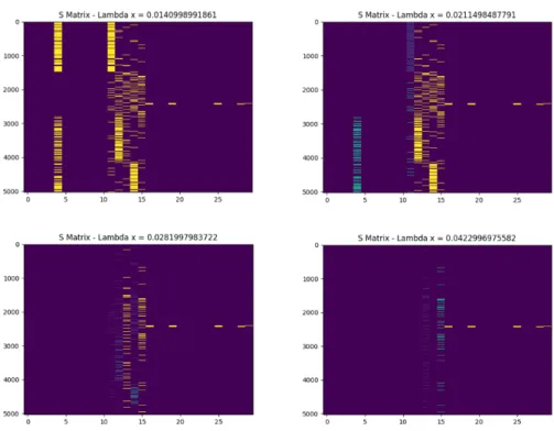
5.4 imShow visualizations. These four plots depict sparse S (anomaly) matrices that change as the value ofλincreases. This shows how the coupling constant alters which data points are classified as anomaly and which are normal. Asλis increased the sparse matrices lose entries in their matrices, thus the plots appear to have less data [47]. . . 30

5.5 Initialµandρtesting . . . 31

5.6 _µand_ρtesting after feature generation . . . 31

(11)

LIST OFFIGURES

5.8 Singular values of S matrix from RPCA [21]. This plot has a steep downward trend which is due to the S matrix being sparse and therefore having few entries greater than 0. The result of this is a matrix that has very few dominant singular values which influences the data points in the anomaly matrix [28]. . . 33 5.9 S matrix imShow plot after RPCA. Visualize representation of anomaly S matrix. The

spareness of this results in few data points being represented in this plot [28]. . . 34 6.1 This figure provides an example of PCA dimension reduction. The data points above

are from a subset of data with no attacks or anomalies. The data appears to fit into a 2-dimensional subspace, even though the data exists in a 3-dimensional space. By using PCA, the majority of the data, the green points, can be reduced to a new 2-dimensional subspace. Once this new subspace is produced, the green points have a very low error margin between one another. The red data points, which exit outside of the new 2-dimensional subspace, are determined to be anomalous, as they lie outside of the majority of the data set. Note: this image is an example of PCA dimension reduction, was not a part of this project, and the true data lies in a much higher dimensional space. [55] . . . 40 6.2 This figure provides an example of data in a 3-dimensional space that cannot be

reduced to a lower dimension, showing that truly random data cannot be projected to a lower subspace. [55] . . . 41 6.3 The figure provides an example of RPCA dimension reduction. The given data is the

same as the previous example, a subset of data existing in a 3-dimensional space. Similar to the previous example, an implementation of PCA would result in a new 2-dimensional subspace in the green plane. However, the majority of the data appears to fit a 1-dimensional subspace, even though the given data exists in a 3-dimensional space. RPCA is robust to outliers, and could detect a lower 1-dimensional subspace on which the majority of the data lied. The red data points are regarded as anomalous by both PCA and RPCA in this example, however RPCA was able to recognize purple data points as slightly anomalous in this new 1-dimensional subspace. This is an example of how RPCA is more effective at dimension reduction than PCA. Note: this image is an example of RPCA dimension reduction, was not a part of this project, and the true data lies in a much higher dimensional space. [55] . . . 44 8.1 Home page that display original raw logs. . . 59 8.2 Anomaly matrix table produced by RPCA. . . 59 8.3 tSNE visualizations. Left is tSNE ran on our feature set. Right is tSNE ran on the S

matrix produced by RPCA. . . 60 8.4 Depicts the tooltip for M and M-S Values. M is the original values and M-S is the

(12)

LIST OFFIGURES

8.5 Color scale that portrays warnings, here the larger the S value, the darker the back-ground color. . . 63 8.6 Viewing VAST firewall log data in our web application . . . 63 8.7 Date Selectors in application. Here you would choose dates to run RPCA on a specified

time slice. . . 64 8.8 Visualization of RPCA anomaly matrix in web application. . . 64 8.9 Example of how M and M-S values are depicted. . . 64 8.10 Undocumented computer attack shown in anomaly matrix. Here we cross validated

that our features found this attack by referencing the ground truth. . . 65 8.11 tSNE visualization using our features. To the left is the visualization with our features

and to the right is post-RPCA . . . 66 8.12 Flowchart of tSNE result creation. One of our goals in closing the loop in an anomaly

(13)

(14)

C

H A P T E R

1

I

NTRODUCTION

By Guth, Sola, and Velarde

1.1

Introduction

It would be difficult to speak on the successes of technology in past years without discussing the recent attacks on user data. The data explosion from technological growth has armed analysts with new strategies for predicting or detecting malicious activity. Taking data from previous attacks can help us prevent or stop future ones from emerging. This method of preventing attacks can be summarized as finding outliers in a data set – or an anomaly. An anomaly is a data point that veers away normal trends in a data set. From credit card fraud detection to cybersecurity at-tacks, detecting anomalies has become vital in ensuring privacy. Nevertheless, due to differences between data in these domains, a generalized solution for detecting out of the ordinary behavior becomes challenging. In this paper, we will focus on anomaly detection in cybersecurity of the 2011 VAST dataset challenge.

Between the Internet of Things, the rapid advancement of technology and the lack of regula-tion in the past years, security has become a primary concern for millions of users. In addiregula-tion, anomaly detection in networks has various layers of mathematical complexity. Deciding which data points seem out of place requires precise analysis of data. This, coupled with the enormous size of data sets, subtle correlation between data points, and potential long system waits for each run cycle makes the process known as feature engineering non-trivial [9].

Security issues have been steadily present in software companies as technology continues to grow in use and complexity. Considering how heavily embedded technology has become in every-day life, cybersecurity is an issue of the highest priority. Damage costs alone from cyber attacks are projected to reach $6 trillion by 2021 and breaches of personal information are occurring with higher frequency as time progresses [53]. Over the past years, government records have been victimized of cyber attacks, for example, the Free Application for Federal Student Aid (FAFSA)

(15)

CHAPTER 1. INTRODUCTION

experienced a security breach within its IRS retrieval application. This led to roughly 100,000 taxpayers information being compromised [6]. As time and technology progresses, malicious infiltrations such as the FAFSA breach become increasingly more difficult to predict or detect. To protect user information, avoid denial of service attacks, along with other types of infiltration, it is vital to detect what has gone wrong in the past regarding security. Determining the root cause of these issues assist improving the security of critical information and user privacy.

Anomaly detection has been researched extensively for cybersecurity due to the complexities that it entails. The University of Minnesota’s, Anomaly Detection: A survey, looked at using network intrusions detection systems to find anomalies. However, detecting anomalous behavior through network data comes with several challenges. This type of dataset is inherently high dimensional and the domain continuously changes over time as intruders adapt and overcome intrusion detections advancements [23].

In this Major Qualifying Project (MQP), we examined ways to diversify a dataset through feature engineering and analyze its relationship with Robust Principal Component Analysis (RPCA). Our contributions were the following:

• Created a user-friendly visualization system.

• Closed the loop between feature generation, mathematical analysis, and visualization. • Improved overall experience of system administrators by creating a streamlined process

through careful construction of sound infrastructure in our code base.

This report explains in depth what anomaly detection is, its process, the different statistical analysis methods that we will use or recommend to use, what feature engineering is, and the impact that the original data set we used had on our project along with the assumptions made.

(16)

C

H A P T E R

2

VAST D

ATASET

C

HALLENGE

By Sola and Velarde

For this project, we used the 2011 VAST dataset [5]. This dataset included network architec-ture descriptions, security policy issues, firewall logs, an intrusion detection system (IDS) log, and a Nessus Network Vulnerability Scan Report [27] for the All Freight Corporation (AFC) [5]. The goal of the challenge was to develop situation awareness interfaces that provide insight quickly, clearly, and as efficiently as possible to help manage daily business operations while mitigating network vulnerabilities. In this chapter, we will explain the structure of AFC’s network and the associated dataset.

2.1

2011 VAST Dataset

Feature engineering refers to the process of using knowledge of data to create features that can make machine learning algorithms function [52]. More specifically, this refers to attributes that could contribute to the analysis of data to help with its prediction or analysis. Features are characteristics of data that will help distinguish each row of data from each other. For example, a feature would be whether or not a log entry is using a port that has a specific type of vulnerability. This feature becomes relevant as we know that attacks are more likely to come from a computer that might be vulnerable. In general, features surround the balance between finding as much relevant data as possible to ensure that it is unique enough to make an impact in the prediction models.

The dataset includes a folder of firewall logs for four separate days April 13 - 16 of 2011. Each day has one corresponding log file. However, in the instance that the number of rows exceeds Excel’s row limit multiple files are created. April 13 is such a case, where there exists more than one log file. There are certain nodes within the dataset that are critical for AFC’s network to function properly. It is to be noted that AFC uses virtual machines within their network. In

(17)

CHAPTER 2. VAST DATASET CHALLENGE

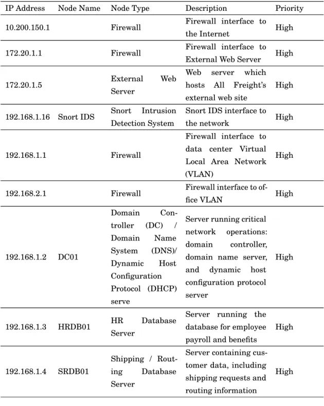
table 2.1, all nodes are described in the VAST dataset challenge; any node outside 172.x.x.x and 192.x.x.x is external to AFC’s network.

IP Address Node Name Node Type Description Priority 10.200.150.1 Firewall Firewall interface to

the Internet High 172.20.1.1 Firewall Firewall interface to

External Web Server High

172.20.1.5 External Web Server

Web server which hosts All Freight’s external web site

High

192.168.1.16 Snort IDS Snort Intrusion Detection System

Snort IDS interface to

the network High

192.168.1.1 Firewall

Firewall interface to data center Virtual Local Area Network (VLAN)

High

192.168.2.1 Firewall Firewall interface to

of-fice VLAN High

192.168.1.2 DC01 Domain Con-troller (DC) / Domain Name System (DNS)/ Dynamic Host Configuration Protocol (DHCP) serve

Server running critical network operations: domain controller, domain name server, and dynamic host configuration protocol server

High

192.168.1.3 HRDB01 HR Database Server

Server running the database for employee payroll and benefits

High

192.168.1.4 SRDB01

Shipping / Rout-ing Database Server

Server containing cus-tomer data, including shipping requests and routing information

(18)

2.1. 2011 VAST DATASET

192.168.1.5 WEB01 Internal web server

Server that hosts All Freight’s corporate in-tranet, including com-pany news site and pol-icy and procedure man-uals

High

192.168.1.5 WEB01 Internal web server

Server that hosts All Freight’s corporate in-tranet, including com-pany news site and pol-icy and procedure man-uals

High

192.168.1.6 EX01 Mail server

Server that stores and routes all email that flows into, out of, or in-ternal to All Freight

High

192.168.1.7 FS01 File Server

Server that holds shared files used by workers throughout All Freight

High

192.168.1.14 DC2 DC / DNS server

Server running critical network operations: domain controller and domain name server

High

192.168.1.50 Firewall log Server that captures

system firewall logs High 192.168.2.10 through 192.168.2.250 Office worksta-tions Individual worksta-tion computers located in offices or cubicles throughout All Freight

Normal

Table 2.1:AFC registered network description. [5].

Important data flow descriptions are: • Connections outside of the AFC network

– Web traffic enters with IP address 10.200.150.1 and through port 80.

– Firewall routes traffic to the external web server on 172.20.1.5 address and through port 80.

(19)

CHAPTER 2. VAST DATASET CHALLENGE

• Email from outside AFC network

– Enter AFC’s network with IP address 10.200.150.1 through port 25.

– Firewall routes traffic to the mail server on IP address 192.168.1.6.

• All AFC staff members use IP addresses 192.168.2.10-250 to browse the internet.

All information above retrieved from VAST dataset challenge description. Fully understand-ing the structure of a dataset and how data flows in AFC’s network is critical to the success of this project and taken into consideration during its execution. In general, a company’s policy and security contract should be taken into consideration when creating features.

2.2

Attacks in the VAST Dataset

In addition to the resources mentioned above, the VAST dataset also includes a solutions manual. The answer guide reveals all attacks and steps that led to finding the security vulnera-bilities in the VAST dataset. Below are summaries of each attack over the course of four days according to the solution manual.

Type of Attack Date of Attack Description Denial Of Service Attack

(DDoS)

04/13/2011 at 11:39 and ended roughly an hour later at 12:51

A DDoS attack aims to dis-rupt a user’s interaction with a system. By using client/server technology an attacker can flood requests of a network, rendering that network use-less or experiencing delayed speeds [62]. Throughout this time period there was an at-tempt to disrupt a corporate web server, most likely to de-lay network speeds.

(20)

2.3. AVOIDING DATA SNOOPING

Remote Desktop Connection 04/14/2011 at 13:31 Documented violation of cor-porate policy within the fire-wall logs. This is part of a so-cially engineered attack that suggests substantial security risk such as a worm in AFC’s network.

Undocumented Computer 04/14/2011 13:23 There was an addition of an undocumented computer in the company internal net-work. The policy descriptions for AFC said that the work-station computers would be in the range 192.168.2.25-250. The particular IP address for this computer is 192.168.2.251. Although we do not have the background for this computer, the addition of it to the com-pany network is concerning enough that it should be no-ticed.

Table 2.2:Attack Descriptions on VAST dataset [5]

2.3

Avoiding Data Snooping

Data snooping is when an algorithm can cheat through previous knowledge of the answers rather than depend on how data presents itself normally. We used the context of the attacks mentioned above to verify the validity of our features and assist with the iterative feature engineering process. One of our primary concerns of having the answers was the possibility of data snooping. Although we did take inspiration from knowing the attacks and previous MQPs, we limited ourselves to not seeing the answers until we had our first iterations of features. After observing the answers, we analyzed the problems in general to create features that would have the capabilities to solve these issues in a generalized way. For example, when we noted the Remote Desktop attack, we thought about all different types of protocols that could indicate that a computer is being connected from a suspicious place and how ports can hint at suspicious activity.

(21)

CHAPTER 2. VAST DATASET CHALLENGE

2.4

Previous Work

In the previous year, there was an MQP that focused on an anomaly detection system. After analysis of their work, we determined that their application was set up in a way that created a disconnected loop of work between mathematicians and computer scientists. From the computer science side, there were matrices of features developed and sent to mathematicians for analysis. These matrices were derived from the 2011 VAST dataset challenge. It was important to determine how their features were produced from this data.

After a code analysis, we determined that the VAST 2011 dataset was ingested into a Python script and then the resulting feature matrix was inserted into a mySQL [10] database. The mySQL tables were statically defined, meaning that the table schema was established during the creation of the feature matrix with a predetermined set of columns. We believe that this posed a problem for a generalized solution. Our initial thought was to research ways of dynamically creating the table schema for the mySQL table. To do this, we chose to optimize the process of running the project and feature matrix creation. Our Python script allowed the feature matrix to be read for mathematical analysis and from here, rows were marked as anomalous or not. This was done with the ground truth from the solution manual and served for cross validation of attacks. The main problem with the previous MQP project was the disconnect between each step in the iterative loop, this needed to be streamlined. With the past MQP’s structure of feature generation and math analysis, we chose to close the loop that began with feature engineering, passed to mathematical analysis, and resulted in visualization.

(22)

C

H A P T E R

3

A

NOMALIES IN

C

YBER

S

ECURITY

By Sola and Velarde

The exponential increase of technology in the past years has made malicious intrusions in networks substantially harder to detect anomalies. The heavy integration of technology into our lives has made detecting intrusions all the more important [24]. Anomaly detection involves looking at previous data and searching for behavior that exists out of the norm. Anomaly detection methods create the possibility to find unknown attacks on a system once a normality has been defined. However, false positives are still possible due to the unpredictable nature of network use.

3.1

Anomaly detection methods

Anomaly detection is the process of finding data that is out of the ordinary and does not conform to previous data trends [23]. The difficulty levels to find anomaly corresponds to the layers of complexity a dataset provides.

In Figure 3.1, it is obvious to see that there are points that do not behave as the rest of the data. It is important to note that in this example there are only two dimensions. In a real world example there can be multiple dimensions. Each dimension adds another layer of complexity and can affect or even hide anomalous behavior [23]. One example is network data and traffic. Network data consists of communicating with multiple computers or nodes [45]. Figure 3.2 is an example of how complex network traffic can look in comparison to the simple example above.

In Figure 3.2, we see multiple systems communicating with each other. Each node in this diagram represents a layer of complexity in a network. Finding behavior that is out of the norm with everything taken into consideration very quickly becomes a daunting task. With more data ingested at a fast rate, data becomes noisy and harder to filter through. Regarding network data it is vital to filter through this noise. “Network traffic anomalies reflect the anomalous or malicious

(23)

CHAPTER 3. ANOMALIES IN CYBER SECURITY

Figure 3.1:Example of anomaly in two dimensional space [23].

Figure 3.2:Example of dimensionality in network traffic. Each node represents another layer of complexity. This makes detecting anomalies a non-trivial task [23]

behaviors that appear in the network. Discovering exact/actual network traffic anomalies is to effectively contain these anomalous or malicious behaviors that damage the network” [76]. These network traffic anomalies communicate a story of attacks in cyber security and it is the responsibility of anomaly detection methods to ensure that they are caught and examined. The question that many experts are posing is which anomaly detection methods are best and how can we better prepare ourselves for unknown attacks [14].

Different project paradigms require different types of anomaly detection methods [23]. Testing different types of anomaly detection methods can result in an increased chance of finding anomalous behavior [14]. In recent years, the different types of anomaly detections methods have skyrocketed. This stems from advancements in technology and an increase in targetable domains [14]. The challenge lies in identifying the correct type of anomaly detection method (ADM) for a

(24)

3.1. ANOMALY DETECTION METHODS

domain. Many anomaly detection methods have different requirements and prerequisites that can makes the process even more difficult. Below is a general architecture for an anomaly detection system.

Figure 3.3:General architecture of anomaly detection system from (Chandola et al., 2009) [23]

Although Figure 3.3 is a generalized example of an anomaly detection system, it accu-rately describes the steps that are taken into consideration for examining a dataset. The actual anomaly detection engine is what will normally vary. There are several examples of anomaly detection methods. Monowar H. Bhuyan, D. K. Bhattacharyya, and J. K. Kalita’s [23] paper mentioned above categorizes network intrusion methods into the following categories: statistical, classification-based, clustering and outlier-based, soft computing, knowledge-based and combina-tion learners. Most of these anomaly deteccombina-tion methods use some form of feature engineering to optimize their anomaly detection algorithms. Bhuyan, Bhattacharyya, Kalita argue that “feature selection reduces computational complexity, removes information redundancy, increases the accuracy of the detection algorithm, facilitates data understanding and improves generalization” [14]. It is therefore, important that the feature selection process is carefully chosen based on a dataset.

(25)

C

H A P T E R

4

F

EATURE

E

NGINEERING

By Sola and Velarde

Feature engineering is analyzing data to carefully separate data points in a useful way. The goal is to diversify and create meaningful distances between data points. To be more specific, when analysts first receive data, it might have what seems as redundant or not specific enough information. As stated in chapter 3, feature selection enhances anomaly detection algorithms. In order to choose which data points are anomalies, you have to select which details need to be analyzed, and most importantly, how. One of the challenges about data mining is the different perspective that a user or analyst can have in comparison with a developer. Looking at the problem domain from two different perspectives can derive to a different set of features. [69].

4.1

Feature Engineering Process

The process of feature engineering is an iterative one that ceases when the end goal of a project is met. The process is defined below by Dr. Jason Brownlee [19]:

1. Preprocess Data: Format it, clean it, sample it so you can work with it.

a) This may involve deleting certain columns after determining any irrelevancies. b) Changing the format of certain columns, such as time-stamps or unwanted characters. 2. Transform Data: Feature selection happens here.

a) The feature library consists of several uniquely identifying characteristics of the data. b) Features should not be made for the sake of creation. For example, a timestamp

feature would diversify your data; however, that might not help you achieve your goal. 3. Model Data: Create models, evaluate them and fine tune them.

(26)

4.2. FEATURE SELECTION FOR A DATASET

a) After receiving results from the feature selection, how will you visualization or present your findings? How can the transformed data set be modeled to communicate a message?

b) Ensure that your features tell a story within your modeling of data.

Through each iteration of this process more is revealed about a dataset and features are fine tuned until a best fit is found. The best fit varies for each project. Overall, it is important to consider if features are thoughtfully chosen and if through the modeling of features a story is clearly communicated.

4.2

Feature Selection For a Dataset

What specifically defines a feature is what makes feature engineering both challenging, and interesting. Intuitively, one may think of a feature as system functionality that helps characterize the system in the perspective of a human. However, this definition tends to be perceived in different ways, causing confusion and conflicting opinions [69]. Using the time entry of a data point, for example, could be considered a feature because it makes each log entry into a separate data point. Nevertheless, this does not necessarily describe the system or how it works. A separate challenge with feature engineering is the limit of file sizes. Although in an ideal world, you could create a feature for each uniquely identifying characteristic, it’s imperative to consider what is possible with the current computational power, and prioritize which features may lead to solving a problem. The selection of features is a task which requires an analytical approach. A dataset must be examined to define which characteristics should be made unique. As mentioned above, choosing the wrong features will not help in the modeling of a dataset and can hinder the problem that feature engineering aims to solve. In the feature selection step is it vital to remove attributes of data that may make a dataset “noisy” and skew any modeling while limiting the number of features to those of higher importance [19].

4.3

Time Series Feature Generation

Although features tend to describe characteristics of a specific dataset, anomaly searching can require an introspective view of your specific domain. Network security has unique attributes that are imperative towards understanding how the network itself is functioning. Osman Ramadan [57], decided to use the number of distinct source and destination ports/IP’s and the sum of bytes for each source over a period of time as features since he knew that this could describe a change in the network’s normal behavior, like a DDoS attack [57]. Our dataset did not include the exact number of bytes transferred within each request. However, in light of his findings we decided to see if it would be possible to derive a similar concept. How could we analyze when a

(27)

CHAPTER 4. FEATURE ENGINEERING

source/destination port/ip was experiencing a change in the network? Questions such as these are key to help us derive rules for modeling data and create our anomaly detection system.

4.4

Feature Engineering Generation

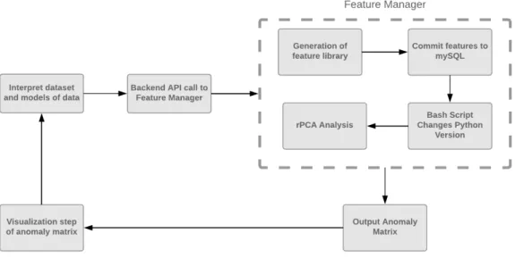
In the following sections we will discuss the process of our feature generation on the VAST dataset. The goal was to generate a set of features that increases uniqueness among the dataset in preparation for mathematical analysis, such as RPCA. Over the course of the project’s completion we followed the iterative process defined above. Below is an example of the loop that resulted in our feature library. In this section, we also explain the workflow of the project. We will go in depth for each step and the part it played in closing the loop in this MQP.

Figure 4.1:A goal of this project was to create a system that closes the loop between an anomaly detecting system and visualization.

Once this cycle has converged as a result of an optimal feature set, the next step is visualiza-tion. This step will be described in depth in chapter 7.

4.5

Feature Generation Infrastructure

In the following sections, the process of choosing our features for the VAST dataset will be described. This section aims to explain the flow of work that led to the efficient generation of our feature library. As described above, a challenge that lies in feature generation is the size of the dataset. In the VAST dataset, with all 4 days of logs, there are roughly 12.5 million rows. Through trial and error, it was determined that we could not feasibly automate and streamline

(28)

4.6. SOURCE AND DESTINATION IP ADDRESS FEATURE SETS

the feature generation process with the entire dataset. Processing the data would require very long system waits for feature generation. To mitigate this problem, a Python script functions as a manager for all of the scripts that produce our feature library. Our backend is created using Flask [59], a micro-web framework written in Python to build our web application. This manager is used within our Flask backend explained in chapter 7, and our web application to obtain a desired time slice for a specific log file. This makes it much more manageable to generate features and test different slices.

Our manager also bears the responsibility of running mathematical analysis. It assists with easy experimentation of our algorithm, as explained in chapter 4. It is to be noted that feature generation occurs with Python 2.7 and math analysis uses Python 3.6. There are ways to translate Python 2 to Python 3 with libraries such as Futurize [64] but with several moving components in our code base and not anticipating this problem in the beginning of the project we decided to not convert our code. One could imagine, that with time, a manager could be written entirely in one Python version or one that utilizes the something such as the Futurize library. As with many Python projects, we decided to develop from within a virtual environment using Python’s VirtualEnv [15]. We took advantage of this decision and have two Python virtual environments, one for Python 2.7 and one with Python 3.6. All dependencies are clearly defined within our code repository readme [65]. Our manager begins feature generation code in the Python 2.7 virtual environment and a bash script is started once feature generation is complete. This bash script deactivates the Python 2.7 virtual environment, activates the Python 3.6 environment to run our math algorithm on the feature matrix csv file. This process closes the gap between computer science and mathematical analysis. What follows is the visualization step of the results for a user, this is explained in more detail in Chapter 6. A user can use this manager and examine any number of ranges for any log. Another advantage of having a manager script is that adding or removing specific feature sets become infinitely easier.

Since the feature generation process is an iterative one that constantly aims to improve in order to optimize the anomaly detection algorithm, creating a pipeline for this project was necessary. This pipeline allowed us to test several different time slices and assisted with the best fit convergence of our feature library.

4.6

Source and Destination IP Address Feature Sets

The goal output of our features is to create a hot encoded matrix in Excel, or a numerical value to demonstrate if a characteristic applies to the data point [45]. It is difficult to apply anomaly detection methods if the features are not chosen carefully. In our features, every IP address was converted to an integer using Python’s struct library. In this section we will describe the trials of deciding how to diversify the IP addresses within the dataset.

(29)

CHAPTER 4. FEATURE ENGINEERING

4.6.1 Original Feature For Every Unique Source and Destination IP

We used a script in order to find every unique source and destination IP address and we dynamically generated features from this. This script examined a user specified slice of the dataset and generated all of the corresponding distinct IP addresses. From here our feature manager starts another script that will create the feature matrix with respect to these distinct IP addresses. All IP addresses are converted to integers as explained above. Source IP addresses have the prefix "sip_" followed by the integer IP address and destination IP addresses have the prefix "dip_" followed by the integer IP address. Below is an example of how the source IP addresses may be displayed within this specific feature set.

sip_18091791 sip_18091792 sip_18091793 sip_32322361 sip_32322362

0 0 0 0 1

1 0 0 0 0

Table 4.1:Original IP Address feature example. In this feature set, there is a columns for every distinct IP address.

This matrix is then inserted into a mySQL table for easy manipulation of data. For example, join in each IP address to a vulnerability scan is one example that can be used in feature generation that would require that flexibility. By having each unique source and destination IP address be its own feature we diversify the dataset and widen our matrix. However, it is important to note the impact that doing this could have on the math analysis and other overall infrastructure of our project. If a user defines a very large time slice of the dataset, the dynamically created features could number in the thousands. This makes it difficult to insert data into mySQL and make queries on it since the table would become so large. For example, if we run our script to generate features for every distinct source and destination IP address, along with our other features, our table would have upwards of a thousand features. In addition, this feature set can hurt the goal of anomaly detection if most of the used IP addresses are unique, since our math algorithm could potentially flag each row as an anomaly. It can be argued that with smaller slices this is a very feasible feature set and can help the diversification of the dataset.

4.6.2 Feature Engineering of the AFC Network IP Addresses

As mentioned in chapter 2, the VAST 2011 dataset challenge included a table of IP addresses that describes the AFC company network architecture.

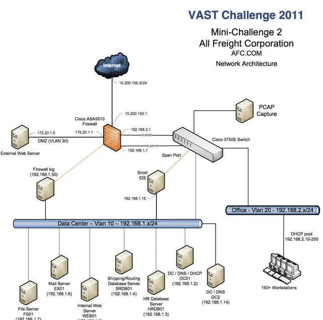
Figure 3.3, maps the overall transfer and communication of data within AFC’s network. All of the IP addresses in this figure are referenced in chapter 2’s table. Our next IP address feature

(30)

4.6. SOURCE AND DESTINATION IP ADDRESS FEATURE SETS

Figure 4.2:AFC Network Architecture. This outlines the workstation connections in AFC’s network and which servers they communicate on. [5]

(31)

CHAPTER 4. FEATURE ENGINEERING

set includes the thoughtful consideration of exclusively AFC’s network. For each IP address in table 2.1 we have a source and destination feature. Similarly to the previous section’s feature set, we prefix each IP address with "sip_" and "dip_" and convert each address to an integer. In addition, there are two features responsible for characterizing any source or destination IP addresses outside of AFC’s defined network called "sip_outside" and "dip_outside". Below is an example of how these features look.

sip_outside sip_18091777 sip_18091793 sip_32322361 sip_32322362

0 0 0 0 1

1 0 0 0 0

Table 4.2:Individual Column features for each AFC network IP address. With this feature set, there is a column for every IP address defined in AFC’s network and there are two columns for source and destination IP addresses outside the defined network.

There may be several reasons for communication with an outside IP address, however, it is important to mark these IP addresses as they could be the root of malicious activity. In a real world setting, one could imagine speaking with a network analyst at any given company and asking for a similar network architecture diagram or table. By doing this, someone could use our software and place their own IP addresses in a simple table in our Python script and run their own feature generation. This is where our goal of a more generalized solution for anomaly detection is accomplished. In the previous section, the features change from each feature generation run cycle, but in this situation the feature set for IP addresses stay the same. This feature set encompasses the entire AFC network architecture.

By mapping out each IP address in AFC’s network as a feature we characterize their company specific architecture. This could make identifying specific workstations or other terminals as a problem quite simple. As for marking outside sources the outside features can alert any source or destination IP address that is external to the AFC network. In the next section we aim to generalize the IP addresses even further.

4.6.3 Examining AFC Network IP Addresses Inside and Outside

This IP address features is a slight variation of the previous section. We wanted to try another version of examining AFC’s network architecture. This set includes four features in total: "sip_outside", "sip_inside", "dip_outside", and "dip_inside". Rather than having a feature for

(32)

4.7. PORTS

each IP address, we use these features and simply marked whether an IP addresses is in a user defined slice is inside or outside the AFC network. Below is an example of how these features look.

sip_outside sip_inside dip_outside dip_inside

0 1 0 1

Table 4.3:Examining only inside and outside source and destination IP addresses according to AFC’s network architecture.

It was important to test several variations for the IP address features because this attribute in the firewall log can tell an interesting story when it comes to suspicious activity. For the "sip_inside" and "dip_inside" features we still ingest the AFC network architecture similar to the previous section. However, in this set we consolidate all of those features into these two columns. So every IP address defined in AFC’s network will be placed within those two columns. The "sip_outside" and "dip_outside" functions the same as the previous section where all IP addresses that are outside of AFC’s network will be marked there.

4.7

Ports

Ports can reveal much about abnormalities in network data. For this reason we found it necessary to incorporate them into this project’s feature library. We created features for the ports and grouped them according to overall significance to possible malicious attacks. Port numbers below 1024 are known as system or well-known ports. They are specifically meant to be used for certain applications and the system expects them to perform certain tasks. On the other spectrum, ports above 1024 are ports and they can be used by users or are registered. An example is how the 8080 port is registered for websites. For our features, we grouped all port numbers. Unique source ports below 1024 all have their own column with a prefix, "special_source_port_" followed by the port number. All other source ports above 1024 are grouped into a separate column. For the destination ports, we also had two different grouping. Normally, a destination port will be port number 80. Port 80 is used for web servers and "listens" to a client. Since, there is a high chance that port 80 would be used frequently for destination ports we created a column for rows that used port 80. We then classified each destination port that is not 80 as a special destination port. We created a separate column of those ports with prefix, "special_destination_port_" followed by the port number.

(33)

CHAPTER 4. FEATURE ENGINEERING

In addition,we investigated ports that usually served a program or signaled a type of danger. For example, port 3389 corresponds to the TCP and UDP ports that are used for Microsoft’s remote desktop, software that you would not necessarily expect in a non-tech company. In addition, we looked at strategic ports used by hackers or malicious software to have a wider range of ports that could signal an attack. In the table below is a list of the ports that is included in our features.

Port Description/Threat

3389 Remote Desktop Protocol (RDP) - Ports that allows a user a graphical interface to connect to another computer for Windows.

6783-6785 Remote Desktop Protocol (RDP) SplashTop 53 DNS Exit Strategy and port used to create

DDOS attacks.

4444 Trojan to listen in on information

31337 Back Orifice backdoor and some other mali-cious software programs

6660 - 6669 Internet Relay Chart (IRC) Vulnerabilities & DDoS

12345 Netbus Trojan Horse 514 Explotable Shell

Table 4.4:Examined ports for feature generation. These ports have been exploited in years past and could indicate a threat [1], [2], [72].

It was important to tag these ports as they could be critical to alerting a system administrators of possible malicious behavior.

4.8

Averages

An interesting detail about network traffic, is that it is comprised of several layers to make itself efficient and secure. Though normally one would examine packages sent and received to characterize a network flow, that information is not always readily available. The VAST Dataset did not include this; therefore, we needed to emulate how a network would work with the data that we had available.

In order to develop a feature that encompassed anomalous numbers of requests, we had to develop a feature that could encapsulate what a “regular” amount of requests were, and what we considered to be out of that range. We considered this for source IP addresses, destination IP addresses, source ports, and destination ports. We will refer to these as network parameters in this section. To do this, we calculated the average of the network parameter requests per

(34)

4.8. AVERAGES

second. This would be able to detect if a parameter was used more or less than normal during a certain time period. Doing so is critical to detecting attacks such as a DDoS attack. Each second has a certain number of requests per parameter. For example, if you have an IP address as the parameter, 192.0.0.1, and it appears three times in a period of one second, that is three requests per second. Below are the steps that our Python script completes to calculate this feature.

1. Individually examine each second in the dataset as a slice 2. Retrieve the requests per second for each network parameter 3. Calculate average based on the network parameter

4. For each second for a network parameter divide it by the average requests per second For each of the parameters mentioned above, a mySQL table is defined with the schema depicted in table 4.5.

Field Type Null Key

date_time varchar(34) No Primary [parameter] varchar(34) No Primary Appearance per

Sec-ond

varchar(34) Yes

Final_Feature varchar(34) Yes Final_Work_Feature varchar(34) Yes

Table 4.5: Average feature set table schema. This feature attempts to emulate the amount of requests each network parameter made.

Since the table would be nearly identical, except the network parameter, we created a template for the table creation. Similarly to the working set mySQL table, explained in chapter 4 section 5, these tables are defined each time that the feature manager is ran with a different time slice. It is important to note that these slices are not representative of the global dataset, but rather, a just the slice a user chooses. There were a few reasons why we decided to keep these features local rather than global. The last average feature’s purpose is to capture a significant change in the network. If we used the global data, a DDoS attack, for example, could skew the data since it will completely change the total work done by a system. Examining the slices locally can imitate a real world system by analyzing a fixed number of logs, and as they come in the last average feature theoretically would be able to capture the change. Finally, there was also a memory component in the generation of the features. If we decided to use global data, in a real time system it would need to be periodically updated when new logs come in, and it would increasingly need more memory. By maintaining the logs locally, we reduce the amount of memory needed and have much more efficient process to creating the features.

(35)

CHAPTER 4. FEATURE ENGINEERING

In addition, a second feature was generated that looked at the amount of work that a specific address or port generated of the total amount of work done in the system during that time. Although the process is similar to retrieve the current work for the address/port, the difference is that instead of dividing by the average work done, we divide by the total. What this accomplishes is that it contrasts what we consider an above average address/port for the system with what the total work on the system is done. Table 4.6 shows how our features were represented.

Source IP LastAver-age

Destination IP Las-tAverage

Source Port LastAver-age

Destination Port Las-tAverage

1.00 1.28 1.00 0.20

1.83 4.16 1.00 1.00

2.45 2.83 1.00 2.28

Table 4.6:Average feature example.

4.9

Vulnerability Scan Analysis

The vulnerability scan used was generated from a Nessus scan [27]. Nessus is a vulnerability scanning platform, used mainly by security analysts. The Nessus vulnerability scan offers information regarding a system’s health and if there are areas that malicious hackers could utilize to cause harm. A parser [40] was used on the Nessus scan provided in the VAST dataset to extract information relevant to our feature generation. Among these relevancies are the note, hole, and Common Vulnerability Scoring System (cvss) parameters. Notes represent a security warning and are indicators of behavior that is slightly out of the norm. A hole is representative of a larger security warning, often critical to system health [27]. The cvss value ranges from 0 to 10 and provides further insight into the severity of these health warning indicators. Below is an example of the vulnerability scan used before parsing.

Count Note Count Hole Max Severity Note Max Severity Hole

1 0 1 0

51 209 2.6 9.3

Table 4.7:We use the Nessus scan [27] to validate features. Here we examine the amount of notes and holes per IP address.

To efficiently query IP addresses that could potentially be the root of a critical vulnerability, the parsed values were stored in a mySQL table. Table 4.8 shows the schema of this table in mySQL:

(36)

4.9. VULNERABILITY SCAN ANALYSIS

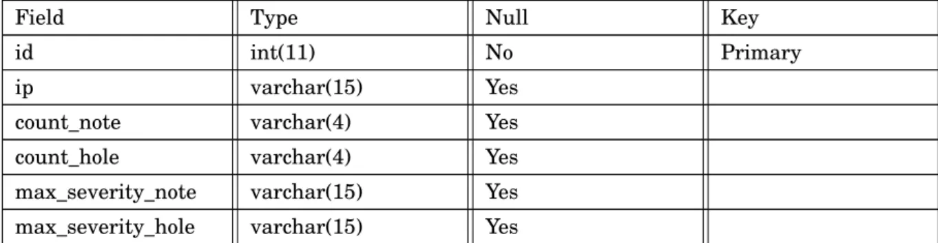
Field Type Null Key

id int(11) No Primary ip varchar(15) Yes

count_note varchar(4) Yes count_hole varchar(4) Yes max_severity_note varchar(15) Yes max_severity_hole varchar(15) Yes

Table 4.8:Nessus Scan table schema. We used this table to join firewall logs and vulnerability scan information.

Once the table is populated with these values it is joined with the mySQL features table. The join occurs according to the IP address. The result is the features table with the addition of these four vulnerability scan features. With these features it is simple to see exactly which IP addresses are causing problems and will allow us to validate the accuracy of the formerly mentioned features.

Features themselves focus on describing the data set rather than finding anomalies [36]. To find anomalies using features, we depend on learning algorithms, which are used as a part of machine learning to process information and determine patterns for a given dataset [3]. In the next chapter, we will discuss different learning algorithm techniques and how they can affect anomaly detection [3].

(37)

C

H A P T E R

5

L

EARNING

A

LGORITHMS By Guth

Once feature generation was completed, the data could be exported for mathematical analysis. The extracted information was analyzed through statistical methods in an attempt to analytically detect anomalies in the dataset. Various parameters were tested and produced results that accurately detected anomalies when comparing the mathematical results to the ground truth network data.

5.1

Supervised and Unsupervised Learning

There are many statistical methods that could be used as we are looking for relationships between characteristics of network logs to find discrepancies and anomalies. Many statistical methods were evaluated to help determine what would fit best for the network data being analyzed, including different types of learning algorithms. Supervised learning includes statistical approaches where possible results are already known, and the data being analyzed is labeled with correct answers [33]. On the contrary, unsupervised learning algorithms can analyze data to find patterns and relationships that might not have been known or examined before [30]. Principal Component Analysis (PCA) is an unsupervised statistical approach used for data dimension reduction and processing [79]. This is done by taking a data set of observations and converting them to a set of linearly uncorrelated principal components for further analysis. By using a Singular Value Decomposition (SVD), a given matrix M_∈Rm×ncan be broken down as follows: [26]

M₌UΣVT

where U_∈Rm×n _{is a unitary matrix,}_Σ

∈Rn×n which is a positive definite diagonal matrix with zeros elsewhere, and V_∈Rn×n, also a unitary matrix [26]. The diagonal entriesσi∈Σare known

(38)

5.2. SINGULAR VALUES

as the singular values ofM, are similar but not always the same as eigenvalues. Singular values are only equivalent to eigenvalues when the given matrix is real, symmetric, square, positive definite matrix. As stated, PCA can be used for dimension reduction and to project matrices onto a lower dimensional subspace, which would work well for finding anomalies within network data. PCA unfortunately suffers from each principal component being a linear combination of all original observations, making it difficult to interpret results and susceptible to outliers.

5.2

Singular Values

For the first subset of network data that was analyzed after preprocessing what was done, the resulting matrix of network data logs was M_∈R5034×34_{. There were initially four logs in the}

matrix that returned undefined for the IP addresses, which resulted in these rows being deleted from the matrix as to not interfere with the analysis. Then, for an SVD to be produced for this matrix, the first four columns of the matrix had to be ignored. These columns were id, destination IP, source IP, and time log, and were not of values that could be computed for the new matrices. This resulted in the matrix being trimmed down to a size of 5034 by 34, at which point the matrix was factorized as an SVD producing the results below.

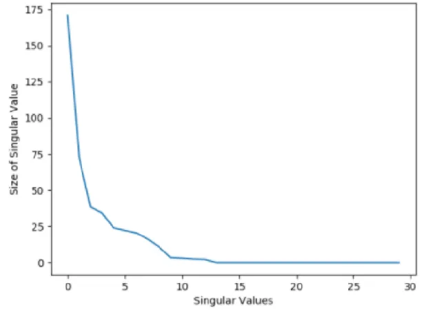
TheΣmatrix contained 30 unique singular values (σi) [21], corresponding to the 30 columns

in our adjusted matrix . Theseσivalues declined in weight as they were expected to, and only the

first 13_σ_ivalues returned coefficients above zero. This means that with the largest 13 singular values, we have the ability to predict the other 17 singular values for any log we’re given, allowing us to predict the remaining information and details of an individual log if we know less than half of it’s information. The 30_σ_ivalues can also be seen below in descending order. After the results were produced, more analysis was done on the logs and columns of the network data that were being produced. The matrices of network data were of size 1000000 by 34 for the first 12 csv files that were exported, and the 13th csv file contained slightly fewer logs of data, meaning there were slightly less than 13 million logs of data to iterate through. The 13 unique network data csv files were read and concatenated into a singular data matrix, with the first four columns being ignored, which was then z-Transformed and processed into an SVD the same way our subset sample of data had been. The z-Transformation process is described later in section 5.4 of this paper.

Using the first two singular values of theΣmatrix, every log in the concatenated csv files were plotted by using the first two singular values of the Σ matrix as the xand yaxis. The columns of the csv files were also plotted by the same convention, using the first two singular values of theΣas the axis for plotting. The first two singular values were selected above the rest because the results of theΣmatrix are returned in descending order, so the first two singular values represent the two values that scale the U andVT unitary matrices of the SVD to recreate the original matrix.

(39)

CHAPTER 5. LEARNING ALGORITHMS

Figure 5.1:Visual representation of the singular values of the first time slice of data. Singular values appear in descending order due to the construction of the SVD andΣ[21].

The first two singular values were then multiplied by the U unitary matrix, returning a vector of slightly less than 12 million rows by 2 columns in size. This was also done to theVT

unitary matrix, of which the results were transposed to be in the same form as the other product. The columns of the two products of U andVT respectively were then separated into arrays, the values were sent to lists, and the lists were then zipped together to create the data points that would be plotted. Once the values for the U andVT by the first two singular values plots were generated, they were produced with the results below.

The singular values by U graph displayed all logs within the concatenated matrix of all 13 network data csv files, which displays a somewhat linear relationship between the data, with individual data points falling above and below a general trend line. The singular values byVT

graph displayed the columns of the concatenated matrix of all 13 network csv files, with each point in the plot representing a different column. These columns were expected to be less linearly dependent on one another than the log data, because the columns of the matrices represent the features of each individual data point, where there was clearly disparity between many of the logs and respective features.

(40)

5.3. ROBUST PRINCIPAL COMPONENT ANALYSIS

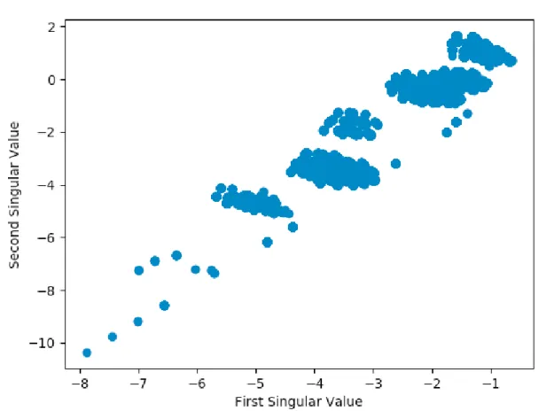
Figure 5.2: Singular Values by U. This displays a loose linear relationship between all data points. The first two singular values were chosen to be the axes because those are the two most dominant values to help predict other features of an individual log [21].

5.3

Robust Principal Component Analysis

Robust Principal Component Analysis (RPCA) is an adjusted statistical approach of PCA which works with corrupted observations and outliers [28]. While PCA is susceptible to outliers as previously stated, RPCA can detect a more accurate low dimensional space to be recovered, and that is why RPCA is necessary over standard PCA for anomaly detection in the network data. RPCA works to recover a low-rank matrix L and a sparse matrix S from corrupted measurements, which in the case of network data would be the anomalies of the data set. Robust PCA works in conjunction with the Singular Value Decomposition (SVD) factorization method of separating matrices into distinct unitary and diagonal matrices, giving an optimization problem as follows: [28]

min(L,S)||L||∗+λ||S||1

(41)

CHAPTER 5. LEARNING ALGORITHMS

Figure 5.3:Singular Values by VT. The spareness of the plot shows how there is no apparent linear relationship between the columns or features of the dataset [21]. This is logical because features are linearly independent of each other. For example, IP addresses and ports do not depend on each other.

In this equation, L is the low rank matrix which can be factorized as an SVD,_||L_||_∗is the nuclear norm of L (the sum of the singular values),λis the coupling constant between L and S,

||S_||₁is the sum of the entries S, and_εis the matrix of point-wise error constants that improve the noise generated from real world data. Due to the nature of the network data, traditional PCA would be too receptive to outliers and would prove to be ineffective and anomaly detection. As a result, RPCA was the statistical method chosen for anomaly detection.

5.4

Z-Transform

Due to having various different types of information that were created through the feature generation process, data normalization was necessary. Between the source and destination ports, source and destination IP addresses, and averages that were calculated for when certain IP addresses and ports came up throughout the dataset, a z-Transformation of the data was

(42)

5.5. λ

necessary as a preprocessing method before further analysis could be done. This was in each column of the matrices that were generated, and was done by using the z-score statistical method. [51]

z₌(x−µ)

σ

For each column in the data set, the meanµ and standard deviationsσof a given column were calculated. If the_σof a given column was not zero, each individual data point in the column was taken, had theµ of the column subtracted from the given point, and that sum was then divided by theσof the total column. If theσof a given column was zero, this would have resulted in division by zero for all points in the column and would have produced NaNs (not a number), denoting infinities and numbers that could not be read for further analysis. This was done for all columns of data in the matrices that were generated, and these new z-Transformed matrices were exported as new pandas dataframes for future use. After the z-Transformation was completed, the new data matrix was evaluated as a numpy SVD (Singular Value Decomposition) to generate the singular values of the z-Transformed data of the original given matrix.

5.5

λ

One of the most crucial variables to RPCA is _λ, the coupling constant between the low dimension L and S matrices, where L and S sum together to create the original matrix used for analysis [28]. The L matrix in this case is an SVD of the non-anomalous data, and the S matrix is a sparse matrix that represents the data points from the original matrix that are found by RPCA to be anomalous.λis the variable that differentiates what is considered anomalous, what is not, and controls what is allowed into the S matrix. Ifλis small, more data points will be allowed to move from the L matrix to the S matrix, and as_λincreases fewer data points will be considered anomalous. The theoretical value ofλis equal to the following:

[47]

λ=p 1

max[m,n]

wheremandnrepresent the rows and columns of the original matrix. For this project,_λ was altered from the default value in an attempt to improve the capabilities of RPCA in finding anomalous entries within network data. This was done by changing the numerator value of one to a integer variable, and then changing the variable many times to see the differences between the L and S matrices as lambda was changed. This was done on a chosen small slice of data from the network data set and was analyzed as a 5000 by 30 matrix. This equation can be seen below, whereHis the integer variable in change_λ:

[47]

λ=p H

(43)

CHAPTER 5. LEARNING ALGORITHMS

Figure 5.4: imShow visualizations. These four plots depict sparse S (anomaly) matrices that change as the value of_λincreases. This shows how the coupling constant alters which data points are classified as anomaly and which are normal. Asλis increased the sparse matrices lose entries in their matrices, thus the plots appear to have less data [47].

By using the matplotlib [29] imShow function, the following plots were produced to provide visuals of how the entries in S were changing asλwas altered. A few examples of the imShow plots can be seen below, where it can be seen that fewer entries appear in the S Matrix imShow plots as the value of_λis increased.

5.6

µ

and

ρ

Two other variables used in RPCA are mu_µ and rho_ρ, which are used in the augmented Lagrangian parameter that are used for convergence testing. The theoreticalµandρare taken fromThe Augmented Lagrange Multiplier Method for Exact Recovery of Corrupted Low-Rank Matrices[46] and are used in conjunction with given epsilon εvalues to act as the stopping criterion to help determine whether the RPCA code is converging based on the matrix it was given. The default_µand_ρare respectively:

[46]

µ= 1 ||D_||₂

(44)

5.6. µANDρ

where,_ρs=_mn|Ω|

Where _||D_||2 represents the spectral norm (largest singular value) of the given matrix D,

andρs acts as the sampling density betweenρandρs. For this project,µandρwere altered

from their default value in an attempt to improve the capabilities of RPCA and improve the convergence rate of given matrices being tested. Two time slices were chosen from the network data of size 5000 by 30 and 50000 by 526 respectively after features generation. The tables below show how the convergence rate of a given matrix was changed afterµandρwere changed, using the theoreticalλvalue for all tests run. As seen in Figure 5.5 and 5.6, theµandρvalues of 0.05 and 1.05 respectively greatly improved the number of iterations needed for RPCA to meet it’s given stopping criterion. These values were deemed to be an improvement over the theoretical values [46] as a result.

Figure 5.5:Initialµandρtesting

(45)

CHAPTER 5. LEARNING ALGORITHMS

5.7

Implementing RPCA

After tests were done on the first subset of data, a larger subset of data was chosen to test on. The second subset of data contained network logs from the DDoS attack, and after ignoring the non-discrete columns of the matrix the size was 50000 by 526. This matrix was z-Transformed and factorized as an SVD, and its singular values were calculated accordingly [28]. However, this matrix was also run through RPCA, which produced different singular values due to the matrix being projected to a lower dimensional space. The matrix was decomposed into the form

M₌L₊S, whereL₌UΣVT is factorized as an SVD and S represents the sparse anomaly matrix of the given matrix M [28]. The plots of the original singular values, the RPCA singular values, and the imshow plot of the sparse anomaly S matrix, which depicts what cells are regarded as anomalous, are shown in Figures 5.7. 5.8, and 5.9.

(46)

5.7. IMPLEMENTING RPCA

Figure 5.8:Singular values of S matrix from RPCA [21]. This plot has a steep downward trend which is due to the S matrix being sparse and therefore having few entries greater than 0. The result of this is a matrix that has very few dominant singular values which influences the data points in the anomaly matrix [28].

(47)

CHAPTER 5. LEARNING ALGORITHMS

Figure 5.9:S matrix imShow plot after RPCA. Visualize representation of anomaly S matrix. The spareness of this results in few data points being represented in this plot [28].

After the manager, described in section 4.5 (Feature Infrastructure) was fully set up, mathe-matical analysis tests became much easier to run for different feature s

Anomaly Detection Using Robust Principal Component Analysis

Worcester Polytechnic Institute

Repository Citation

PROFESSORS LANE HARRISON, RANDYPAFFENROTH

List of Figures vii

TABLE OF CONTENTS

TABLE OF CONTENTS

LIST OFTABLES

FIGURE Page

LIST OFFIGURES

LIST OFFIGURES

Introduction

CHAPTER 1. INTRODUCTION

VAST D

2011 VAST Dataset

CHAPTER 2. VAST DATASET CHALLENGE

2.1. 2011 VAST DATASET

CHAPTER 2. VAST DATASET CHALLENGE

Attacks in the VAST Dataset

2.3. AVOIDING DATA SNOOPING

Avoiding Data Snooping

CHAPTER 2. VAST DATASET CHALLENGE

Previous Work

Anomaly detection methods

CHAPTER 3. ANOMALIES IN CYBER SECURITY

3.1. ANOMALY DETECTION METHODS

Feature Engineering Process

4.2. FEATURE SELECTION FOR A DATASET

Feature Selection For a Dataset

CHAPTER 4. FEATURE ENGINEERING

Feature Engineering Generation

Feature Generation Infrastructure

4.6. SOURCE AND DESTINATION IP ADDRESS FEATURE SETS

Source and Destination IP Address Feature Sets

CHAPTER 4. FEATURE ENGINEERING

4.6.2 Feature Engineering of the AFC Network IP Addresses

CHAPTER 4. FEATURE ENGINEERING

4.6.3 Examining AFC Network IP Addresses Inside and Outside

Ports

CHAPTER 4. FEATURE ENGINEERING

Averages

4.8. AVERAGES

CHAPTER 4. FEATURE ENGINEERING

Vulnerability Scan Analysis

4.9. VULNERABILITY SCAN ANALYSIS

Supervised and Unsupervised Learning

5.2. SINGULAR VALUES

Singular Values

CHAPTER 5. LEARNING ALGORITHMS

5.3. ROBUST PRINCIPAL COMPONENT ANALYSIS

Robust Principal Component Analysis

CHAPTER 5. LEARNING ALGORITHMS

Z-Transform

CHAPTER 5. LEARNING ALGORITHMS

CHAPTER 5. LEARNING ALGORITHMS

Implementing RPCA

5.7. IMPLEMENTING RPCA