Balancing Load in Stream Processing
with the Cloud
Wilhelm Kleiminger
#1, Evangelia Kalyvianaki
∗2, Peter Pietzuch
∗3 #Department of Computer Science, ETH Z¨urichUniversit¨atstrasse 6, 8092 Z¨urich, Switzerland 1[email protected]
∗Department of Computing, Imperial College London
180 Queen’s Gate, South Kensington Campus, London SW7 2AZ, United Kingdom 2[email protected] 3[email protected]
Abstract— Stream processing systems must handle stream data coming from real-time, high-throughput applications, for example in financial trading. Timely processing of streams is important and requires sufficient available resources to achieve high throughput and deliver accurate results. However, static allocation of stream processing resources in terms of machines is inefficient when input streams have significant rate variations— machines remain underutilised for long periods of average load. We present acombinedstream processing system that, as the input stream rate varies, adaptively balances workload between a dedicatedlocalstream processor and acloudstream processor. This approach only utilises cloud machines when the local stream processor becomes overloaded. We evaluate a prototype system with financial trading data. Our results show that it can adapt effectively to workload variations, while only discarding a small percentage of input data.
I. INTRODUCTION
Today’s information processing systems face difficult chal-lenges as they are presented with new data at ever-increasing rates [1]. Especially in the financial industry, high volume streams of data have to be processed by high-throughput systems in order to derive accurate statistics for modelling the markets. For example, for 7 days in November 2010, the average data rate from a NYSE market data feed was 1.3 Mbps with 123.7 Mbps during bursts [2].
Stream processing systems are fundamentally different from ordinary data management systems. Streams are infinite and important events are sparse [3]. This means that data has to be processed by continuous queries and results made available on-the-fly. In contrast to batch-processing systems, the size of the processed data is not constant but determined by the arrival rate of the input stream. These processing demands encourage stream processing systems to be distributed across multiple machines [4].
In financial data streams, tuple arrival times are not uniform during a trading day. At certain times, the workload peaks at a multiple of the average load. Since a typical trading day is from 8am to 4pm, it is less economically efficient to dedicate resources that cover peak loads for 24 hours a day, 7 days a week. Traditionally, stream processing systems use load shedding when the workload exceeds their processing
capabilities [5]. This employs a trade-off between delivering a low-latency response and ensuring that all incoming tuples are processed. However, load shedding is not feasible when the variance between peak and average workload is high. A system that must discard the majority of tuples is of limited use when accurate processing is needed.
Ideally, a stream processing system should be self-adapting by load balancing in order to handle changes in the work-load. To avoid load shedding, we propose to distribute the computational load of stream processing in a way that utilises a scalable cluster infrastructure in a cloud computing service such as Amazon EC2 [6]. Our goal is to provide a scalable local stream processor that automatically streams a partial data stream across a high bandwidth network channel to a cloud service when local resources become insufficient. By fully utilising the local processor and only processing data in the cloud on demand, the cost and energy consumption of stream processing can be reduced.
Achieving parallel stream processing in a cloud environment with good performance is challenging. In general, complex queries allow for higher throughput through parallelisation. A complex query can often be broken down into a series of steps that construct a pipelined job. However, when it comes to window size, the solution is not quite as clear. The size of the input window is usually specified by the query. It can be variable if the query refers to a timespan (time-based window) or constant if it specifies a number of tuples (count-based window). A large window may be split across multiple machines using a divide-and-conquer approach such as MapReduce [1]. This is only feasible for complex queries with large windows. As windows become smaller, parallelisation at tuple granularity (data parallelism) introduces too much overhead. Small windows must be processed at window granularity.
In this paper, we present a combined stream processing system that balances load between a local stream processor and a distributed stream processor running on a scalable cloud infrastructure. We describe an adaptive load balancing algo-rithm that is capable of distributing the input stream at between the local and the cloud stream processors. The cloud stream
processor supports stream partitioning at tuple granularity and at window granularity to parallelise the processing task. We evaluate the system using a realistic financial processing workload and show that the main factor in load balancing stream processing with the cloud is the bandwidth between the load balancer and the cloud data centre.
In the remainder of this paper, we first discuss related work in the next section. We introduce our approach for stream processing with cloud resources in Section III. In Section IV, we explain the load balancing algorithm used to support the local stream processing. We evaluate the performance our system in Section V and draw conclusions in Section VI.
II. BACKGROUND
Scalable stream processing. Previous work on stream processing has explored the parallel execution of queries. STREAM is a data stream management system (DSMS) de-veloped by Arasu et al. [7]. It uses the Continuous Query Language (CQL)—an extension of SQL. Queries are evaluated by translating them to a physical query plan that is processed by the DSMS. The distribution of the query can be achieved through placement of operators across multiple machines.
The Mortar stream processor [3] is geared towards pro-cessing of data from sensors. It uses an overlay network and distributes the operators over a tree to increase fault-tolerance. It supports a large number of stream sources, but there is no provision for peak load scenarios as encountered in financial data processing. Mortar supports in-network operators to re-duce the amount of information sent over the network. Similar pre-processing can be done by our load balancer to increase throughput. We compress data before sending it to the cloud processor, but further bandwidth optimisations such as filtering are possible.
Cayuga [8] is an event processing system for handling complex streaming data. A simple extension to Cayuga scales stream processing by partitioning queries over n machines using row/column scaling [9]. Tuples can be routed in a round-robin fashion to different rows. However, this does not preserve dependencies for stateful queries. This approach is similar to our window-granularity approach for the simple cloud stream processor. We distribute windows over a column of processors to make efficient use of multiple machines.
Load balancing. Research on load balancing has focused on data locality. Pai et al. [10] use a single load balancer that receives requests from clients for static web content. The content is stored on a number of back-end web servers. The load balancer examines a request for a particular resource and routes it to the server with the least load. In a stream processing system, the roles are reversed because the query is fixed. The load balancer has to deal with allocating the data. This requires a robust load balancing algorithm that takes bandwidth and latency constraints into account, as well as, the processing time of the stream processor in order to utilise fully the local node and a remote cluster.
Cloud
Load balancer
Stream provider Client
Local stream processor
Processed window Unprocessed window
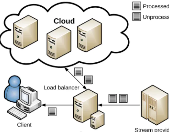
Fig. 1. Overview of combined stream processing system.
Randles et al. [11] compare different load balancing strate-gies in cloud computing. The emphasis lies on making the best use of resources. For example, the “honeybee forag-ing” algorithm probes available resources and advertises their capabilities on a distributed shared-space address board. By calculating the profitability of the individual servers (i.e. how quickly they can serve a request), the system can adjust load. Unprofitable resources are abandoned while the profitable ones are allocated more tasks. However, this assumes an envi-ronment with heterogeneous resources—in a homogeneous cloud data centre, we can assume that the capabilities of the participating nodes are known in advance. In our approach, a dedicated node in the cloud handles the reception of jobs from the load balancer.
III. CLOUD STREAM PROCESSING
We describe acombinedstream processing system that uses a local stream processor to handle average loads while utilising cloud resources when faced with peak demand. The goal is to ensure efficient usage of resources for any given workload, while offering acceptable throughput and reliable processing of data.
A typical stream processing query over stock market data could notify a user about a particular stock exceeding a limit (e.g. the user is interested if Schlumberger (SLB) shares rise above $60). However, more complex composite queries are possible—the user could ask to be notified about the aforemen-tioned rise only if Royal Dutch Shell (RDS-A) shares dropped at the same time. This is achieved by continuously processing a windowof financial data from these two companies. A window is defined as a set of tuples. Each tuple signifies an event—in this case, a change in the price of a share. The size of the window is determined either by a time interval (i.e. has the share price changed within the last 10 minutes), or by the specification of a tuple count. A window can be seen as a unit of work for the stream processor.
Figure 1 gives an overview of our load balancing approach. Our system consists of a front-end node running the local stream processor that handles average load. The distributed cloud stream processing system assists for peak processing
demands and can scale processing across many machines. The stream provider delivers raw data streams to the front-end node. Clients can submit queries to access the stream data. The front-end node runs aload balancerthat is the key component of our system. It dynamically distributes the load between the local processor and the cloud processor. In this way, cloud processing remains transparent to the user. Once stream tuples have been processed by the combined system, a result stream is delivered to the client.
In practice, such an approach requires a high bandwidth network link (e.g. 10–100 Mbps) between the local node and the cloud, otherwise the network is unable to handle bursts in the input data rate as mentioned before. The processing in the cloud is bounded by the number of windows that it receives. If the bandwidth between the local node and the cloud is not sufficient, we can only “outsource” a limited amount of data. These limitations can be overcome partly with techniques such as tuple filtering [12] and compression [13]. Our system uses the zlib compression library to reduce windows sizes prior to transmission, with an observed reduction by a factor of 6 on average.
Cloud Stream Processor.The cloud stream processor consists of a front-end node called a JobTracker and worker nodes called TaskTrackers. Its architecture is inspired by a batch processing system such as MapReduce [1]. In contrast to other stream processing systems [7], we have followed Condie et al. [14] and chosen a simple query semantics using map()and
reduce() functions over the more widely used SQL-like approach. The resulting architecture allows for the seamless addition and removal of resources in a cloud environment.
The map function takes a (key, value)pair and pro-duces a list of pairs in a different domain. These tuples are then grouped under the same key. The resulting tuples of (key, [value]) pairs are processed by the reduce function that produces output values in a (possibly) different domain.
When a user submits a query to the system, it is au-tomatically distributed over all available TaskTrackers. The cloud stream processor manages the addition and removal of TaskTrackers to enable cloud scaling. The input stream is received by the JobTracker and then partitioned over the TaskTrackers. Once the output has been computed, the set of result tuples is sent back to the client through the JobTracker. The cloud stream processor operates at a window granu-larity. Each TaskTracker computes the submitted query over a whole window. If n TaskTrackers are registered with the JobTracker, it is possible to compute nwindows in parallel.
Given a sufficiently large window and a complex query, a cluster of machines can also parallelise the query at tuple granularity. In this case, the JobTracker receives a window, partitions it into equally-sized chunks, and orders the Task-Trackers to use the map andreduce functions for computing the output in parallel. As our experimental evaluation reveals, this approach does not work well because of the small size of the input window, the simplicity of the query and the overhead due the transmission of intermediate results between the nodes. These problems are discussed further in Section V.
Cloud
Processed window Unprocessed window
Load balancer
Local stream processor Stream provider Client Input queue Output queue 1 4 3 2
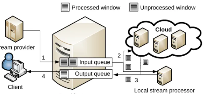
Fig. 2. Queue management performed by load balancer. The numbers show the sequence of steps.
idle local dual
item in queue window dropped
item in queue window dropped
queue empty
queue empty
dropped below threshold item in queue
threshold exceeded
overloaded
Fig. 3. State diagram of transitions between local and cloud-assisted stream processing.
Local Stream Processor. The local stream processor is a simplified version of the cloud stream processor. Similar to the cloud stream processor, the local stream processor uses
map()andreduce()functions to compute the query over the data. Since it communicates with the load balancer over network sockets, it does not have to run on the same node as the load balancer. This means that our load balancer could be used with a different stream processor such asCayuga [8].
IV. ADAPTIVE LOAD BALANCING
When adaptively balancing the workload between the local processor and the cloud processor, we expect the local node to process the stream most of the time. Without load balancing, the local stream processor would have to discard windows when the incoming data rate increases beyond its processing capacity. At this point, the load balancer forwards the excess windows to the cloud processor in order to sustain throughput at an increased input rate.
The operation of the load balancer using multiple queues is illustrated in Figure 2. We assume that the client fulfils a dual role of being both the stream source and consumer of the result stream. Incoming windows are added to aninput queue (step 1). The load balancer monitors the size of this queue to decide when to make use of the cloud processor. Depending on the state of the load balancer, windows are assigned to the local stream processor, or to both, the local and the cloud stream processor (step 2). The output from both stream processors is sent to an output queue(step 3). The output queue is needed to ensure that the output tuples are returned in the correct order. Due to the different processing latencies between the local and the cloud stream processors, windows might have been re-ordered. In step 4, the output windows are sent back to the client.
States diagram.The operation of the adaptive load balancer is controlled according to the state transition diagram in Figure 3. In the initial state, the load balancer isidle. When a window of data is received, it is appended to the input queue and a state transition to thelocalstream processing state occurs. As long as the queue size remains below the threshold sT, the local node can handle the demand and remains in the local state. If the queue becomes empty, the load balancer falls back into the idle state.
The threshold value must take into account processing latency as well as the number of nodes in the cloud. A high threshold means that cloud resources are used only when needed. This reduces the number of state switches and avoids unnecessary costs. However, the latency of the system is dominated by the number of queued windows. In the worst case, the size of the input queue stays constant at sT −1. In this case, the latency for a new window issT×lLwherelLis the processing time of the local stream processor for a single window. In our experiments in the next section, we usesT = 5 because we want to utilise fully the local processor and the 4 nodes in our test-bed cluster acting as the cloud service.
When the queue fills above threshold sT, the load balancer transitions to the dual state. In this state, both the local processor and the cloud processor process the input data. As long as the queue size remains constant, the load balancer stays in this state. A decreasing queue size means that there is spare processing power. However, the balancer returns to the local state only when the queue has been completely drained. This is to ensure that the switching overhead is minimised.
When the input queue overflows even after all available resources in the cloud are used, the load balancer moves to the overloaded state and drops windows to handle the load. In absence of any dropped windows, the load balancer returns to the dualstate.
V. EVALUATION
In this section, we evaluate how the adaptive load balancing scheme performs when supporting the local stream processor with additional capacity from the cloud. Our main goal is to explore how the load balancer uses the cloud resources to handle workload peaks in the input rate effectively without losing any data during periods of transitions.
First we show that window-granularity stream processing in the cloud outperforms the tuple-granularity approach. Then we investigate how much added capacity (in terms of total throughput) the cloud can provide in the combined system. Our results show that throughput is increased and the percentage of dropped tuples lowered by using the adaptive load balancing algorithm.
We consider the following metrics for different input rates: (a) the percentage of dropped tuples with respect to the total number of tuples gives an indication of the efficiency of the load balancer; (b) the throughput increase in the combined stream processing system when utilising the cloud infrastruc-ture; and (c) theCPU and memory utilisationat the local node
200 400 600 800 1000 1200 1400 0 50 100 150 200 250 300 350 400 Number of tuples (1000’s) Time (minutes)
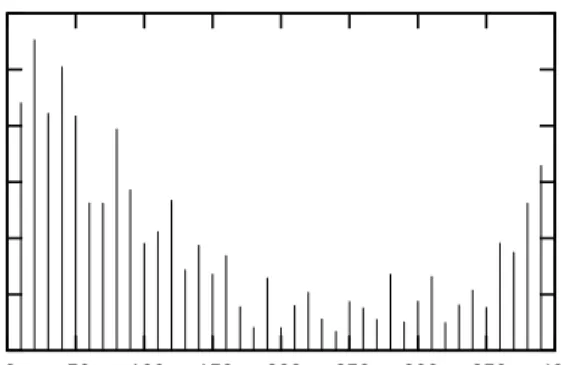
Fig. 4. Tuple arrival rates during single trading day (sampled every 10 minutes).
and cloud nodes. It is desirable to keep nodes fully utilised for economical reasons.
A. Experimental setup
Both local and cloud nodes are AMD Opteron 2346 4-core machines with 4 GB of RAM and are connected by Gigabit Ethernet. In our set-up, the stream provider and client run on the same node to accurately measure total processing latency. They are implemented as a combination of Python and shell scripts. We also monitor resource utilisation of the local stream processor and the load balancer. The CPU utilisation is sampled every second and averaged across a 10 minute window.
Our dataset contains quotes for options on the Apple stock for a single trading day across multiple North American stock exchanges from 8am to 4pm. The total size of the data set is 1.6 GB, divided into 22,372,560 tuples with timestamps. The average tuple arrival time is 777 tuples per second. The average, however, is not characteristic of the actual distribution, which is shown in Figure 4: trading during the morning hours is more intensive. During the first 10 minutes, 2166 tuples arrive at the processor per second on average. This is equivalent to a stream of 173 KB/s. After that arrival time drops continuously until it reaches a trough around midday. Such changes in the arrival rate have implications for load balancing—in this setting, the cloud stream processor must become active immediately to assist in the surge of morning traffic.
Query. We use a realistic stream query that finds pairs of exchanges with the same strike price and expiry data for “put” and “call” options. This information could then be used for put/call parity arbitrage algorithms [15]. Each tuple in our dataset contains 16 comma-separated values including the strike price, expiration day, expiration year, exchange identifier and expiration month code. The first step is to re-order the input tuples to obtain(key, value)pairs with the relevant data:
key = (StrikePrice, ExpDay, ExpYear) value = (Exchange, ExpMonthCode)
TABLE I
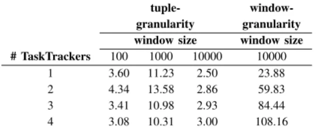
THROUGHPUT(INKB/S)FOR STREAM PARTITIONING AT TUPLE AND WINDOW GRANULARITY.
tuple- window-granularity granularity window size window size # TaskTrackers 100 1000 10000 10000
1 3.60 11.23 2.50 23.88
2 4.34 13.58 2.86 59.83
3 3.41 10.98 2.93 84.44
4 3.08 10.31 3.00 108.16
The list [(key, value)] of key-value pairs is then grouped by key to give the(key, [value])tuples for the reduce function. The reduce function operates on one of these tuples. It ignores the key and finds pairs of exchanges with corresponding put and call options. It starts with the first value in the list and compares it to all other values. If the value is a put option, any matching call options are considered (and vice versa). Once the first entry has been compared to the remainder of the list, it continues with the next entry, ignoring duplicates. This operation is repeated for every key. The complexity of this process is O(n2). The paired exchanges are attached to the keys and returned as a list of(key, [parity])pairs, where
parity = [((Exchange 1, ExpMonthCode 1), (Exchange 2, ExpMonthCode 2))]. The output of the map function is concatenated to give the final output of the algorithm.
B. Tuple vs window granularity
In this section, we compare partitioning at tuple and window granularities, as used by the cloud stream processor to process stream data in parallel. The processing is performed by the TaskTrackers of the cloud stream processor.
We first consider the tuple granularity approach. Table I shows the maximum throughput obtained for different window sizes when increasing the number of TaskTrackers from one to four. For all cases, the data is read directly from disk in order to measure only the processing latency. Increasing the number of TaskTrackers for small window sizes of less than 10,000 tuples reduces the throughput of the system. This is because the communication overhead involved when the TaskTrackers exchange intermediate results is higher than the processing latency of a single TaskTracker. However, our system benefits from larger window sizes (10,000 tuples). In-creasing the number of TaskTrackers improves the throughput up to 20% in the case of four TaskTrackers.
To better understand the cause of this small improvement, we observe the CPU utilisation of the cloud nodes. For two TaskTrackers, most of the CPU time is spent on the JobTracker, with the TaskTrackers idling at around 10% during peak load times. Adding more TaskTrackers results in a similar behaviour where the utilisation is less than 10%. Distributing data by the hash of the input keys and thus avoiding the
Number of TaskTrackers CPU utilisation 1 2 3 4 0 50 100 150 200 250 300 350 JobTracker TaskTracker 1 TaskTracker 2 TaskTracker 3 TaskTracker 4
Fig. 5. CPU utilisation for window granularity.
communication overhead is not possible. The keys during the map and reduce phases are not necessarily identical. Thus, in order to remove the need for communicating intermediate results after the map phase, we ran the map function in the JobTracker. As in our case, the map function merely re-orders the tuples, which can be achieved with little overhead. The benefit was relatively small and only increased the throughput by a factor of 2 for a window size of 10,000 tuples.
In summary, although a larger window improves system scalability, tuple granularity is not efficient—the bulk of the processing time is spent in the JobTracker partitioning tuples. The TaskTrackers remain mostly idle for this simple query and thus do not use cloud resources for increased throughput. Due to the fact that the TaskTrackers are unaware of how the window is split, the intermediate data is always communicated back to the JobTracker after the reduce phase. This explains the difference in the single node runs of the tuple- and window-granularity approaches.
Table I also shows the throughput when partitioning at window granularity. For a window size of 10,000 tuples, the throughput increases significantly with the number of TaskTrackers. Figure 5 shows how the window granularity approach effectively utilises cloud resources as more Task-Trackers are added for parallel processing. Each TaskTracker uses on average between 60% and 80% of available CPU time. For the rest of the evaluation, we use the window granularity approach to process data in the cloud because it scales well with the number of additional cloud nodes executing TaskTrackers.
C. Adaptive load balancing
Next we evaluate the load balancer as it propagates windows to the cloud stream processors and uses more cloud resources with increasing input rates.
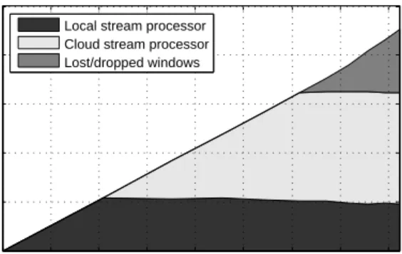
Figure 6 shows the throughput of the combined stream processor with four TaskTrackers when input rates increase. The graph is divided into three areas: (a) the throughput due to the local processor only (lower area of the graph); (b) the throughput due to the cloud processor only (middle area of the graph); and (c) the throughput corresponding to lost/dropped
Input rate (KB/s) Throughput (KB/s) 0 2000 4000 6000 8000 10000 12000 14000 16000 0 50 100 150 200 250
Local stream processor Cloud stream processor Lost/dropped windows
Fig. 6. Tuples processed by the local and cloud processors as input rate increases.
windows (top area). The total throughput of adding (a), (b) and (c) is the throughput under perfect scalability when no tuples are dropped and the input rate can be supported by the network link to the cloud processor. The total throughput of the combined processor is the sum of (a) and (b).
The total throughput of the combined processor increases with the input rate, indicating that our system scales well with increasing load. As the input rates increase, the local processor handles a constant portion of the input data. At the same time, the adaptive load balancer forwards a larger number of windows to the cloud processor—the throughout of the cloud processor increases. At an input rate of 12,000 KB/s, our 4 nodes in the test cloud are overloaded. Since the maximum throughput (see Table I) is reached, windows are discarded.
To scale beyond 4 nodes, we have moved the cloud stream processor to 10 nodes in the Amazon EC2 cloud. With the load balancer running in our university data centre, we have achieved an average processing latency of 2 seconds for a window size of 10,000 tuples. In comparison, by running the cloud system in the aforementioned 4 node scenario, we achieved an average latency of 1 second. We have found the bandwidth between the load balancer and the cloud to be the limiting factor. Even with compression, the throughput achieved by the cloud is limited to 90 KB/s. We believe that further optimisations such as tuple filtering should allow us to use cloud resources more efficiently.
VI. CONCLUSIONS
We have shown that it is possible to construct a combined stream processing system that uses the resources of a cloud infrastructure to assist a local stream processor. The combined approach scales well with increasing input rates by using cloud resources and achieves increased throughput. This is especially relevant for stream processing applications with varying input rates. While adapting to input rates, a small percentage of windows are dropped when the load balancer switches states between local and cloud stream processing to match small periods of burstiness in the arrival rate of input tuples. Our evaluation shows that the combined system is most effective when the input stream is partitioned at a window granularity for parallel processing.
There are several directions for future work. The throughput of the combined system is affected by the quality of the network link between the load balancer and the cloud stream processor. Given our results from the local testbed, we want to explore further tuple compression and leverage pre-processing of the raw stream to reduce bandwidth requirements and thus increase scalability on a cloud service such as Amazon EC2. In our experiments, starting a new instance on EC2 takes well over a minute. This is not fast enough to suit the needs of financial data processing and to build an elastic cloud stream processor. We believe that anticipatory provisioning may help respond to peaks in the arrival time in a timely fashion without dropping windows.
REFERENCES
[1] J. Dean and S. Ghemawat, “MapReduce: Simplified Data Processing on Large Clusters,”Commun. ACM, vol. 51, no. 1, pp. 107–113, 2008. [2] (2010, Nov.) NYSE Euronext Homepage on LatencyStats. [Online].
Available: http://www.latencystats.com
[3] D. Logothetis and K. Yocum, “Wide-scale Data Stream Management,” in ATC’08: Proc. of the USENIX 2008 Annual Technical Conference, Boston, MA, June 2008.
[4] M. Cherniack, H. Balakrishnan, M. Balazinska, D. Carney, U. Cetintemel, Y. Xing, and S. Zdonik, “Scalable Distributed Stream Processing,” inCIDR ’03: Proc. of the Conference on Innovative Data Systems Research, Asilomar, CA, Jan. 2003.
[5] N. Tatbul and S. Zdonik, “Window-aware Load Shedding for Aggrega-tion Queries over Data Streams,” inVLDB’06: Proc. of the 32nd Int. Conference on Very Large Data Bases, Seoul, Korea, Sept. 2006. [6] (2006, Aug.) Amazon homepage on EC2 beta. [Online]. Available:
http://aws.typepad.com/aws/2006/08/amazon ec2 beta.html
[7] A. Arasu, B. Babcock, S. Babu, J. Cieslewicz, M. Datar, K. Ito, R. Motwani, U. Srivastava, and J. Widom, “STREAM: The Stanford Data Stream Management System,” InfoLab, Stanford University, Menlo Park, CA, Technical Report 2004-20, Mar. 2004.
[8] A. Demers, J. Gehrke, M. Hong, M. Riedewald, and W. White, “Towards Expressive Publish/Subscribe Systems,” in EDBT ’06: Advances in Database Technology, ser. LNCS, Y. Ioannidis, M. H. Scholl, J. W. Schmidt, F. Matthes, M. Hatzopoulos, K. Boehm, A. Kemper, T. Grust, and C. Boehm, Eds. Berlin/Heidelberg, Germany: Springer-Verlag, 2006, vol. 3896, ch. 38, pp. 627–644.
[9] L. Brenna, J. Gehrke, M. Hong, and D. Johansen, “Distributed Event Stream Processing with Non-Deterministic Finite Automata,” in DEBS’09: Proc. of the Third ACM Int. Conference on Distributed Event-Based Systems, Nashville, TN, July 2009.
[10] V. S. Pai, M. Aron, G. Banga, M. Svendsen, P. Druschel, W. Zwaenepoel, and E. Nahum, “Locality-Aware Request Distribution in Cluster-based Network Servers,” in ASPLOS ’98: Proc. of the 8th Int. Conference on Architectural Support for Programming Languages and Operating Systems, New York, NY, Oct. 1998.
[11] M. Randles, D. Lamb, and A. Taleb-Bendiab, “A Comparative Study into Distributed Load Balancing Algorithms for Cloud Computing,” in WAINA’10: Proc. of the 2010 IEEE 24th Int. Conference on Advanced Information Networking and Applications Workshops, Perth, Australia, Apr. 2010.
[12] V. Kumar, B. F. Cooper, and S. B. Navathe, “Predictive Filtering: A Learning-based Approach to Data Stream Filtering,” inDMSN’04: Proc. of the 1st Int. Workshop on Data Management for Sensor Networks, Toronto, Canada, Aug. 2004.
[13] A. Reinhardt, M. Hollick, and R. Steinmetz, “Stream-oriented Lossless Packet Compression in Wireless Sensor Networks,” inSECON’09: Proc. of the 6th Annual IEEE Comm. Society Conference on Sensor, Mesh and Ad Hoc Comm. and Networks, Rome, Italy, June 2009.
[14] T. Condie, N. Conway, P. Alvaro, J. M. Hellerstein, K. Elmeleegy, and R. Sears, “MapReduce Online,” EECS Department, University of California, Berkeley, CA, Tech. Rep. 2009-136, Oct 2009.
[15] (2010, Nov.) Understanding Put-Call Parity. [Online]. Available: http://www.theoptionsguide.com/understanding-put-call-parity.aspx/