Local Binary Pattern Features with
Bootstrapped and Weighted ECOC Classifiers
R.S.Smith and T.Windeatt
Abstract Within the context face expression classification using the facial action coding system (FACS), we address the problem of detecting facial action units (AUs). The method adopted is to train a single error-correcting output code (ECOC) multiclass classifier to estimate the probabilities that each one of several commonly occurring AU groups is present in the probe image. Platt scaling is used to calibrate the ECOC outputs to probabilities and appropriate sums of these probabilities are taken to obtain a separate probability for each AU individually. Feature extraction is performed by generating a large number of local binary pattern (LBP) features and then selecting from these using fast correlation-based filtering (FCBF). The bias and variance properties of the classifier are measured and we show that both these sources of error can be reduced by enhancing ECOC through the application of bootstrapping and class-separability weighting.
1 Introduction
Automatic face expression recognition is an increasingly important field of study that has applications in several areas such as human-computer interaction, human emotion analysis, biometric authentication and fatigue detection. One approach to this problem is to attempt to distinguish between a small set of prototypical emo-tions such as fear, happiness, surprise etc. In practice, however, such expressions rarely occur in a pure form and human emotions are more often communicated by changes in one or more discrete facial features. For this reason the facial-action
R.S.Smith,
13AB05, Centre for Vision, Speech and Signal Processing, University of Surrey, Guildford, Surrey, GU2 7XH, UK. e-mail:[email protected]
T.Windeatt,
27AB05, Centre for Vision, Speech and Signal Processing, University of Surrey, Guildford, Surrey, GU2 7XH, UK. e-mail:[email protected]
coding system (FACS) of Ekman and Friesen [8, 19] is commonly employed. In this method, individual facial movements are characterised as one of 44 types known as action units (AUs). Groups of AUs may then be mapped to emotions using a standard code book. Note however that AUs are not necessarily independent as the presence of one AU may affect the appearance of another. They may also occur at different intensities and may occur on only one side of the face. In this chapter we focus on recognising six AUs from the region around the eyes, as illustrated in Fig. 1.
AU1 + AU2 + AU5 AU4 AU4 + AU6 + AU7
Fig. 1 Some example AUs and AU groups from the region around the eyes. AU1 = inner brow raised, AU2 = outer brow raised, AU4 = brows lowered and drawn together, AU5 = upper eyelids raised, AU6 = cheeks raised, AU7 = lower eyelids raised. The images are shown after manual eye location, cropping, scaling and histogram equalisation.
Initial representation methods for AU classification were based on measuring the relative position of a large number of landmark points on the face [19]. It has been found, however, that comparable or better results can be obtained by taking a more holistic approach to feature extraction using methods such as Gabor wavelets or principal components analysis (PCA) [5]. In this chapter we compare two such methods, namely PCA [20] and local binary pattern (LBP) features [14, 1]. The lat-ter is a computationally efficient texture description method that has the benefit that it is relatively insensitive to lighting variations. LBP has been successfully applied to facial expression analysis [16] and here we take as features the individual his-togram bins that result when LBP is applied over multiple sub-regions of an image and at multiple sampling radii.
One problem with the holistic approach is that it can lead to the generation of a very large number of features and so some method must be used to select only those features that are relevant to the problem at hand. For PCA a natural choice is to use only those features that account for most of the variance in the set of training images. For the LBP representation, AdaBoost has been used to select the most relevant fea-tures [16]. In this chapter, however, we adopt the very efficient fast correlation-based filtering (FCBF) [23] algorithm to perform this function. FCBF operates by repeat-edly choosing the feature that is most correlated with class, excluding those features already chosen or rejected, and rejecting any features that are more correlated with it than with the class. As a measure of correlation, the information-theoretic concept of symmetric uncertainty is used.
To detect the presence of particular AUs in a face image, one possibility is to train a separate dedicated classifier for each AU. Bartlett et. al. for example [2],
have obtained good results by constructing such a set of binary classifiers, where each classifier consists of an AdaBoost ensemble based on selecting the most useful 200 Gabor filters, chosen from a large population of such features. An alternative approach [16] is to make use of the fact that AUs tend to occur in distinct groups and to attempt, in the first instance, to recognise the different AU groups before using this information to infer the presence of individual AUs. This second approach is the one adopted in this chapter; it treats the problem of AU recognition as a multiclass problem, requiring a single classifier for its solution. This classifier generates con-fidence scores for each of the known AU groups and these scores are then summed in different combinations to estimate the likelihood that each of the AUs is present in the input image.
One potential problem with this approach is that, when the number positive indi-cators for a given AU (i.e. the number of AU groups to which it belongs) differs from the number of negative indicators (i.e. the number of AU groups to which it does not belong), the overall score can be unbalanced, making it difficult to make a correct classification decision. To overcome this problem we apply Platt scaling [15] to the total scores for each AU. This technique uses a maximum-likelihood algorithm to fit a sigmoid calibration curve to a 2-class training set. The re-mapped value obtained from a given input score then represents an estimate of the probability that the given point belongs to the positive class.
The method used in this chapter to perform the initial AU group classification step is to construct an error-correcting output code (ECOC) ensemble of multi-layer perceptron (MLP) neural networks. The ECOC technique [4, 10] has proved to be a highly successful way of solving a multiclass learning problem by decomposing it into a series of 2-class problems, or dichotomies, and training a separate base classifier to solve each one. These 2-class problems are constructed by repeatedly partitioning the set of target classes into pairs of super-classes so that, given a large enough number of such partitions, each target class can be uniquely represented as the intersection of the super-classes to which it belongs. The classification of a pre-viously unseen pattern is then performed by applying each of the base classifiers so as to make decisions about the super-class membership of the pattern. Redundancy can be introduced into the scheme by using more than the minimum number of base classifiers and this allows errors made by some of the classifiers to be corrected by the ensemble as a whole.
In addition to constructing vanilla ECOC ensembles, we make use of two en-hancements to the ECOC algorithm with the aim of improving classification per-formance. The first of these is to promote diversity among the base classifiers by training each base classifier, not on the full training set, but rather on a bootstrap replicate of the training set [7]. These are obtained from the original training set by repeated sampling with replacement and this results in further training sets which contain, on average, 63% of the patterns in the original set but with some patterns repeated to form a set of the same size. This technique has the further benefit that the out-of-bootstrap samples can also be used for other purposes such as parameter tuning.
The second enhancement to ECOC is to apply weighting to the decoding of base-classifier outputs so that each base base-classifier is weighted differently for each target class (i.e. AU group). For this purpose we use a method known as class-separability weighting (CSEP) ([17] and section 2.1) in which base classifiers are weighted ac-cording to their ability to distinguish a given class from all other classes.
When considering the sources of error in statistical pattern classifiers it is use-ful to group them under three headings, namely Bayes error, bias (strictly this is measured as bias2) and variance. The first of these is due to unavoidable noise but
the latter two can be reduced by careful classifier design. There is often a tradeoff between bias and variance [9] so that a high value of one implies a low value of the other. The concepts of bias and variance originated in regression theory and several alternative definitions have been proposed for extending them to classification prob-lems [11]. Here we adopt the definitions of Kohavi and Wolpert [13] to investigate the bias/variance characteristics of our chosen algorithms. These have the advan-tage that bias and variance are non-negative and additive. A disadvanadvan-tage, however, is that no explicit allowance is made for Bayes error and it is, in effect, rolled into the bias term.
Previous investigation [17, 18, 21] has suggested that the combination of boot-strapping and CSEP weighting improves ECOC accuracy and that this is achieved through a reduction in both bias and variance error. In this chapter we apply these techniques to the specific problem of FACS-based facial expression recognition and show that the results depend on which method of feature extraction is applied. When LBP features are used, in conjunction with FCBF filtering, an improvement in bias and variance is observed; this is consistent with the results found on other datasets. When PCA is applied, however, it appears that any reduction in variance is offset by a corresponding increase in bias so that there is no net benefit from using these ECOC enhancements. This leads to the conclusion that the former feature extraction method is to be preferred to the latter for this problem.
The remainder of this chapter is structured as follows. In section 2 we describe the theoretical and mathematical background to the ideas described above. This is followed in section 3 by a more detailed exposition, in the form of pseudo-code list-ings, of how the main novel algorithms presented here may be implemented (an ap-pendix showing executable MATLAB code for the calculation of the CSEP weights matrix is also given in section 7). Section 4 presents an experimental evaluation of these techniques and section 5 summarises the main conclusions to be drawn from this work.
2 Theoretical Background
This section describes in more detail the theoretical and mathematical principles underlying the main techniques used in this work.
2.1 ECOC Weighted Decoding
The ECOC method consists of repeatedly partitioning the full set of N classes
Ω ={ωi|i=1. . .N} into L super-class pairs. The choice of partitions is repre-sented by an N×L binary code matrix Z. The rows Zi are unique codewords that are associated with the individual target classes ωi and the columns Zj represent the different super-class partitions. Denoting the jth super-class pair by Sj and Sj, element Zi jof the code matrix is set to 1 or 01depending on whether classωihas been put into Sjor its complement. A separate base classifier is trained to solve each of these 2-class problems.
Given an input pattern vector x whose true class c(x)∈Ω is unknown, let the soft output from the jth base classifier be sj(x)∈[0,1]. The set of outputs from all the classifiers can be assembled into a vectors(x) = [s1(x), . . . ,sL(x)]T∈[0,1]L called the output code for x. Instead of working with the soft base classifier outputs, we may also first harden them, by rounding to 0 or 1, to obtain the binary vector h(x) = [h1(x), . . . ,hL(x)]T∈ {0,1}L. The principle of the ECOC technique is to obtain an estimate ˆc(x)∈Ω of the class label for x from a knowledge of the output code s(x)or h(x).
In its general form, a weighted decoding procedure makes use of an N×L weights matrix W that assigns a different weight to each target class and base clas-sifier combination. For each classωiwe may use the L1metric to compute a class
score Fi(x)∈[0,1]as follows: Fi(x) =1− L
∑
j=1 Wij sj(x)−Zij , (1)where it is assumed that the rows of W are normalized so that∑Lj=1Wi j=1 for i= 1. . .N. Patterns may then be assigned to the target class ˆc(x) =arg maxωiFi(x). If the base classifier outputs sj(x)in Eqn. 1 are replaced by hardened values hj(x) then this describes the weighted Hamming decoding procedure.
In the context of this chapterΩ is the set of known AU groups and we are also interested in combining the class scores to obtain values that measure the likelihood that AUs are present; this is done by summing the Fi(x)over allωithat contain the given AU and dividing by N . That is, the score Gk∈[0,1]for AUkis given by:
Gk(x) = 1 NAU
∑
k∈ωi
Fi(x) (2)
The values of W may be chosen in different ways. For example, if Wi j=1Lfor all
i,j then the decoding procedure of Eqn. 1 is equivalent to the standard unweighted L1or Hamming decoding scheme. In this chapter we make use of the CSEP measure [17, 21] to obtain weight values that express the ability of each base classifier to distinguish members of a given class from those of any other class.
In order to describe the class-separability weighting scheme, the concept of a correctness function must first be introduced: given a pattern x which is known to belong to classωi, the correctness function for the jth base classifier takes the value 1 if the base classifier makes a correct prediction for x and 0 otherwise:
Cj(x) = (
1 if hj(x) =Zi j 0 if hj(x)6=Zi j
. (3)
We also consider the complement of the correctness function Cj(x) =1−Cj(x) which takes the value 1 for an incorrect prediction and 0 otherwise.
For a given class index i and base classifier index j, the class-separability weight measures the difference between the positive and negative correlations of base clas-sifier predictions, ignoring any base clasclas-sifiers for which this difference is negative:
Wi j=max 0, 1 Ki
∑
p∈ωi q∈/ωi Cj(p)Cj(q)−∑
p∈ωi q∈/ωi Cj(p)Cj(q) , (4)where patterns p and q are taken from a fixed training set T and Kiis a normalization constant that ensures that the ith row of W sums to 1.
2.2 Platt Scaling
It often arises in pattern recognition applications that we would like to obtain a probability estimate for membership of a class but that the soft values output by our chosen classification algorithm are only loosely related to probability. Here, this applies to the scores Gk(x)obtained by applying Eqn. 2 to detect individual AUs in an image. Ideally, the value of the scores would be balanced, so that a value > 0.5 could be taken to indicate that AUkis present. In practice, however, this is often not
the case, particularly when AUkbelongs to more than or less than half the number
of AU groups.
To correct for this problem Platt scaling [15] is used to remap the training-set output scores Gk(x)to values which satisfy this requirement. The same calibration curve is then used to remap the test-set scores. An alternative approach would have been to find a separate threshold for each AU but the chosen method has the added advantage that the probability information represented by the remapped scores could be useful in some applications. Another consideration is that a wide range of thresh-olds can be found that give low training error so some means of regularisation must be applied in the decision process.
Platt scaling, which can be applied to any 2-class problem, is based on the regu-larisation assumption that the the correct form of calibration curve that maps
clas-sifier scores Gk(x)to probabilities pk(x), for an input pattern x, is a sigmoid curve described by the equation:
pk(x) = 1
1+exp(AGk(x) +B)
(5)
where the parameters A and B together determine the slope of the curve and its lateral displacement. The values of A and B that best fit a given training set are obtained using an expectation maximisation algorithm on the positive and negative examples. A separate calibration curve is computed for each value of k.
2.3 Local Binary Patterns
Fig. 2 Local binary pattern image production. Each non-border pixel is mapped as shown.
The local binary pattern (LBP) operator [14] is a powerful 2D texture descriptor that has the benefit of being somewhat insensitive to variations in the lighting and orientation of an image. The method has been successfully applied to applications such as face recognition [1] and facial expression recognition [16]. As illustrated in Fig. 2, the LBP algorithm associates each interior pixel of an intensity image with a binary code number in the range 0-256. This code number is generated by taking the surrounding pixels and, working in a clockwise direction from the top left hand corner, assigning a bit value of 0 where the neighbouring pixel intensity is less than that of the central pixel and 1 otherwise. The concatenation of these bits produces an eight-digit binary code word which becomes the grey-scale value of the corre-sponding pixel in the transformed image. Fig. 2 shows a pixel being compared with its immediate neighbours. It is however also possible to compare a pixel with others which are separated by distances of two, three or more pixel widths, giving rise to a series of transformed images. Each such image is generated using a different radius for the circularly symmetric neighbourhood over which the LBP code is calculated. Another possible refinement is to obtain a finer angular resolution by using more
than 8 bits in the code-word [14]. Note that the choice of the top left hand corner as a reference point is arbitrary and that different choices would lead to different LBP codes; valid comparisons can be made, however, provided that the same choice of reference point is made for all pixels in all images.
It is noted in [14] that in practice the majority of LBP codes consist of a concate-nation of at most three consecutive sub-strings of 0s and 1s; this means that when the circular neighbourhood of the centre pixel is traversed, the result is either all 0s, all 1s or a starting point can be found which produces a sequence of 0s followed by a sequence of 1s. These codes are referred to as uniform patterns and, for an 8 bit code, there are 58 possible values. Uniform patterns are most useful for texture dis-crimination purposes as they represent local micro-features such as bright spots, flat spots and edges; non-uniform patterns tend to be a source of noise and can therefore usefully be mapped to the single common value 59.
In order to use LBP codes as a face expression comparison mechanism it is first necessary to subdivide a face image into a number of sub-windows and then com-pute the occurrence histograms of the LBP codes over these regions. These his-tograms can be combined to generate useful features, for example by concatenating them or by comparing corresponding histograms from two images.
2.4 Fast Correlation-Based Filtering
Broadly speaking, feature selection algorithms can be divided into two groups: wrapper methods and filter methods [3]. In the wrapper approach different combi-nations of features are considered and a classifier is trained on each combination to determine which is the most effective. Whilst this approach undoubtedly gives good results, the computational demands that it imposes render it impractical when a very large number of features needs to be considered. In such cases the filter approach may be used; this considers the merits of features in themselves without reference to any particular classification method.
Fast correlation-based filtering (FCBF) has proved itself to be a successful fea-ture selection method that can handle large numbers of feafea-tures in a computationally efficient way. It works by considering the correlation between each feature and the class label and between each pair of features. As a measure of correlation the con-cept of symmetric uncertainty is used; for a pair random variables X and Y this is defined as: SU(X,Y) =2 IG(X,Y) H(X) +H(Y) (6) where H(•)is the entropy of the random variable and IG(X,Y) =H(X)−H(X|Y) =
H(Y)−H(Y|X)is the information gain between X and Y . As its name suggests, symmetric uncertainty is symmetric in its arguments; it takes values in the range
[0,1] where 0 implies independence between the random variables and 1 implies that the value of each variable completely predicts the value of the other. In calcu-lating the entropies of Eqn. 6, any continuous features must first be discretised.
The FCBF algorithm applies heuristic principles that aim to achieve a balance between using relevant features and avoiding redundant features. It does this by selecting features f that satisfy the following properties:
1. SU(f,c)>δ where c is the class label andδ is a threshold value chosen to suit the application.
2. ∀g : SU(f,g)>SU(f,c)⇒SU(f,c)>SU(g,c)where g is any feature other than f .
Here, property 1 ensures that the selected features are relevant, in that they are cor-related with the class label to some degree, and property 2 eliminates redundant features by discarding those that are strongly correlated with a more relevant fea-ture.
2.5 Principal Components Analysis
Given a matrix of P training patterns T∈RP×M, where each row consists of a rasterised image of M dimensions, the PCA algorithm [20] consists of finding the eigenvectors (often referred to as eigenimages) of the covariance matrix of the mean-subtracted training images and ranking them in decreasing order of eigenvalue. This gives rise to an orthonormal basis of eigenimages where the first eigenimage gives the direction of maximum variance or scatter within the training set and subsequent eigenimages are associated with steadily decreasing levels of scatter. A probe image can be represented as a linear combination of these eigenimages and, by choosing a cut-off point beyond which the basis vectors are ignored, a reduced dimension approximation to the probe image can be obtained.
More formally, the PCA approach is as follows. The sample covariance matrix of T is defined as an average outer product:
S= 1 P P
∑
i=1 (Ti−m)T(Ti−m) (7)where Tiis the ith row of T and m is the sample mean row vector given by
m=1 P P
∑
i=1 Ti. (8)Hence the first step in the PCA algorithm is to find an orthonormal projection matrix U= [u1, . . .uM]that diagonalises S so that
SU=UΛ (9)
whereΛ is a diagonal matrix of eigenvalues. The columns uqof U then constitute a new orthonormal basis of eigenimages for the image space and we may assume, without loss of generality, that they are ordered so that their associated eigenvalues
λqform a non-increasing sequence, that is:
q<r⇒λq≥λr (10)
for 1≦q,r≦M.
An important property of this transformation is that, with respect to the basis
uq , the coordinates of the training vectors are de-correlated. Thus each uqlies in a direction in which the total scatter between images, as measured over the rows of T, is statistically independent of the scatter in other orthogonal directions. By virtue of Eqn. 10 the scatter is maximum for u1and decreases as the index q increases. For
any probe row vector x, the vector x′=UT(x−m)Tis the projection of the mean-subtracted vector x−m into the coordinate system
uq with the components being arranged in decreasing order of training set scatter. An approximation to x′may be obtained by discarding all but the first K<M components to obtain the row vector
x′′= [x′1, . . . ,x′K]. The value of K is chosen such that the root mean square pixel-by-pixel error of the approximation is below a suitable threshold value. For face data sets it is found in practice that K can be chosen such that K≪M and so this pro-cedure leads to the desired dimensionality reduction. The resulting linear subspace preserves most of the scatter of the training set and thus permits face expression recognition to be performed within it.
3 Algorithms
Section 2 presented the theoretical background to the main techniques referred to in this chapter. The aim of this section is to describe in more detail how the novel algorithms used here can be implemented (for details of already established algo-rithms such as LBP, Platt scaling and FCBF, the reader is referred to the references given in section 2). To this end, Fig. 3 shows the pseudo-code for the application of bootstrapping to ECOC training, Fig. 4 shows how the CSEP weights matrix is cal-culated and Fig. 5 provides details on how the weights matrix is used when ECOC is applied to the problem of calculating AU group membership scores for a probe image.
4 Experimental Evaluation
In this section we present the results of performing classification experiments on the Cohn-Kanade face expression database [12]. This dataset contains frontal video clips of posed expression sequences from 97 university students. Each sequence goes from neutral to target display but only the last image has available a ground truth in the form of a manual AU coding. In carrying out these experiments we fo-cused on detecting AUs from the the upper face region as shown in Fig. 1. Neutral
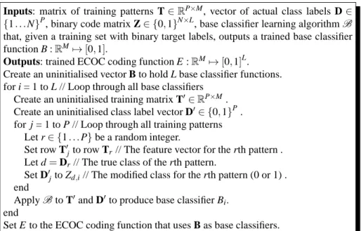
Inputs: matrix of training patterns T∈RP×M, vector of actual class labels D∈ {1. . .N}P, binary code matrix Z∈ {0,1}N×L, base classifier learning algorithmB that, given a training set with binary target labels, outputs a trained base classifier function B :RM7→[0,1].
Outputs: trained ECOC coding function E :RM7→[0,1]L. Create an uninitialised vector B to hold L base classifier functions. for i = 1 to L // Loop through all base classifiers
Create an uninitialised training matrix T′∈RP×M. Create an uninitialised class label vector D′∈ {0,1}P. for j = 1 to P // Loop through all training patterns
Let r∈ {1. . .P}be a random integer.
Set row T′jto row Tr// The feature vector for the rth pattern . Let d=Dr// The true class of the rth pattern.
Set D′jto Zd,i// The modified class for the rth pattern (0 or 1) . end
ApplyBto T′and D′to produce base classifier Bi. end
Set E to the ECOC coding function that uses B as base classifiers.
Fig. 3 Pseudo-code for training an ECOC ensemble with bootstrapping applied.
images were not used and AU groups with three or fewer examples were ignored. In total this led to 456 images being available and these were distributed across the 12 classes shown in Table 1. Note that researchers often make different decisions in these areas, and in some cases are not explicit about which choice has been made. This can render it difficult to make a fair comparison with previous results. For ex-ample some studies use only the last image in the sequence but others use the neutral image to increase the numbers of negative examples. Furthermore, some researchers consider only images with single AU, whilst others use combinations of AUs. We consider the more difficult problem, in which neutral images are excluded and im-ages contain combinations of AUs. A further issue is that some papers only report overall error rate. This may be misleading since class distributions are unequal, and it is possible to get an apparently low error rate by a simplistic classifier that classi-fies all images as non-AU. For this reason we also report the area under ROC curve, similar to [2].
Table 1 Classes of action unit groups used in the experiments.
Class number 1 2 3 4 5 6 7 8 9 10 11 12 AUs present None 1,2 1,2,5 4 6 1,4 1,4,7 4,7 4,6,7 6,7 1 1,2,4 Number of examples 152 23 62 26 66 20 11 48 22 13 7 6
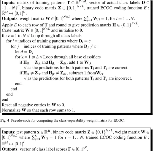
Inputs: matrix of training patterns T∈RP×M, vector of actual class labels D∈ {1. . .N}P, binary code matrix Z∈ {0,1}N×L, trained ECOC coding function E :
RM7→[0,1]L.
Outputs: weight matrix W∈[0,1]N×Lwhere∑Lj=1Wi j=1, for i=1. . .N. Apply E to each row of T and round to give prediction matrix H∈ {0,1}P×L. Crate matrix W∈[0,1]N×Land initialise to 0.
for c = 1 to N // Loop through all class labels for i = indices of training patterns where Di=c
for j = indices of training patterns where Dj6=c let d=Dj
for k = 1 to L // Loop through all base classifiers if Hik=Zckand Hjk=Zdk, add 1 to Wck
// as the predictions for both patterns Tiand Tjare correct. if Hik6=Zckand Hjk6=Zdk, subtract 1 fromWck
// as the predictions for both patterns Tiand Tjare incorrect. end
end end end
Reset all negative entries in W to 0. Normalize W so that each row sums to 1.
Fig. 4 Pseudo-code for computing the class-separability weight matrix for ECOC.
Inputs: test pattern x∈RM, binary code matrix Z∈ {0,1}N×L, weight matrix W∈
[0,1]N×L where∑Lj=1Wi j=1 for i=1. . .N, trained ECOC coding function E :
RM7→[0,1]L.
Outputs: vector of class label scores F∈[0,1]N.
Apply E to x to produce the row vector s(x)∈[0,1]Lof base classifier outputs. Create uninitialised vector F∈[0,1]N.
for c = 1 to N // Loop through all class labels
Set Fc=1−abs(s(x)−Zc)WTc where abs(•)is the vector of absolute compo-nent values.
// Set Fcto 1 - the weighted L1distance between s(x)and row Zc end
Fig. 5 Pseudo-code for weighted ECOC decoding.
Each 640 x 480 pixel image we converted to greyscale by averaging the RGB components and the eye centres were manually located. A rectangular window around the eyes was obtained and then rotated and scaled to 150 x 75 pixels. His-togram equalization was used to standardise the image intensities. LBP features were extracted by computing a uniform (i.e. 59-bin) histogram for each sub-window
in a non-overlapping tiling of this window. This was repeated with a range of tile sizes (from 12 x 12 to 150 x 75 pixels) and sampling radii (from 1 to 10 pixels). The histogram bins were concatenated to give 107,000 initial features; these were then reduced to approximately 120 features by FCBF filtering. An FCBF threshold of zero was used; this means that all features were considered initially to be rele-vant and feature reduction was accomplished by removing redundant features, as described in section 2.4.
ECOC ensembles of size 200 were constructed with single hidden-layer MLP base classifiers trained using the Levenberg-Marquardt algorithm. A range of MLP node numbers (from 2 to 16) and training epochs (from 2 to 1024) was tried; each such combination was repeated 10 times and the results averaged. Each run was based on a different randomly chosen stratified training set with a 90/10 training/test set split. The experiments were performed with and without CSEP weighting and with and without bootstrapping. The ECOC code matrices were randomly generated but in such a way as to have balanced numbers of 1s and 0s in each column. Another source of random variation was the initial MLP network weights. When bootstrap-ping was applied, each base classifier was trained on a separate bootstrap replicate drawn from the complete training set for that run. The CSEP weight matrix was, in all cases, computed from the full training set.
4.1 Classifier accuracy
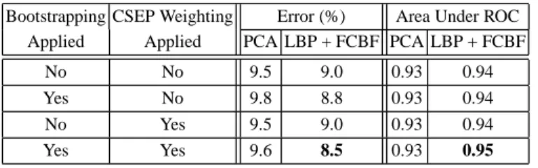
Table 2 shows the mean AU classification error rates and area under ROC figures obtained using these methods (including Platt scaling); the best individual AU clas-sification results are shown in Table 3. From Table 2 it can be seen that the LBP feature extraction method gives greater accuracy than PCA. Furthermore, LBP is able to benefit from the application of bootstrapping and CSEP weighting, whereas PCA does not. The LBP method thus exhibits behaviour similar to that found on other data sets [17], in that bootstrapping and CSEP weighting on their own each lead to some improvement and the combination improves the results still further. By contrast, PCA performance is not improved by either technique, whether singly or in combination. The reasons for this anomaly, in terms of a bias/variance decompo-sition of error, are discussed in section 4.3.
Table 2 Best mean error rates and area under ROC curves for the AU recognition task. Bootstrapping CSEP Weighting Error (%) Area Under ROC
Applied Applied PCA LBP + FCBF PCA LBP + FCBF
No No 9.5 9.0 0.93 0.94
Yes No 9.8 8.8 0.93 0.94
No Yes 9.5 9.0 0.93 0.94
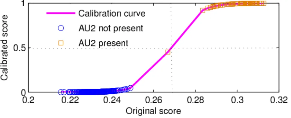
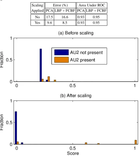
Fig. 6 Calibration curve for AU2 training set (bootstrapping plus CSEP weighting applied).
Table 3 Best error rates and area under ROC curves for individual AU recognition. LBP feature extraction was used, together with bootstrapping and CSEP weighting. MLPs had 16 nodes and 8 training epochs.
AU no. 1 2 4 5 6 7
Error (%) 8.9 5.4 8.7 4.8 11.2 12.3 Area under ROC 0.94 0.96 0.96 0.97 0.92 0.92
4.2 The effect of Platt scaling
As noted in section 2.2, Platt scaling was used to convert the soft scores Gk from Eqn. 2 into approximate measures of the probability that AUkis present. An example of the kind of calibration curves that result from this algorithm is shown in Fig. 6 and the effect of applying the mapping to the test set is shown in Fig. 7. Note that, before calibration all scores are below 0.5 and hence would be classed as AU not present. After calibration (Fig. 7(b)) most of the test patterns that contain AU2 fall to the right hand side of the 0.5 threshold and hence are correctly classified.
Table 4 shows the effect on mean error rates and area under ROC curve. It can be seen that AU detection error rates are approximately halved by this procedure but that it has no effect on the area under ROC curve values. The reason for this is that the application of any monotonically increasing function to Gk does not affect the shape of the ROC curve, it only affects the threshold values associated with each point on the ROC curve.
Table 4 The effect of applying Platt scaling on error rates and area under ROC curves for AU recognition
Scaling Error (%) Area Under ROC Applied PCA LBP + FCBF PCA LBP + FCBF
No 17.5 16.6 0.93 0.95
Yes 9.6 8.5 0.93 0.95
Fig. 7 The effect of Platt scaling on the distribution of test-set scores for AU2.
4.3 A bias/variance analysis
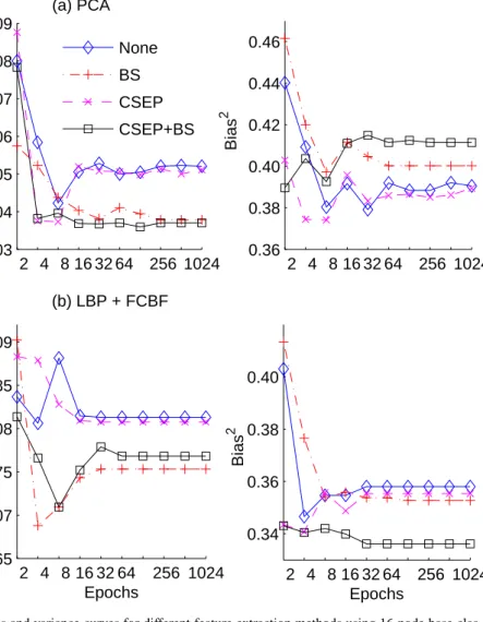
It is instructive to view the performance of these algorithms from the point of view of a bias/variance decomposition of error. Fig. 8 shows bias and variance curves for AU group recognition when the number of training epochs is varied and other parameter settings are fixed at their respective optimal values. It is notable that, for both types of feature extraction, bias error (which, as noted in section 1, includes an unknown amount of Bayes error) predominates. Bias is, however, somewhat higher for PCA (at around 40%) than for LBP (at around 35%). This indicates that LBP is more successful at capturing subtle variations in face expressions than PCA. The downside to this is that LBP feature extraction is more heavily influenced by chance
2 4 8 16 32 64 256 1024 0.03 0.04 0.05 0.06 0.07 0.08 0.09 Variance (a) PCA None BS CSEP CSEP+BS 2 4 8 16 32 64 256 1024 0.36 0.38 0.40 0.42 0.44 0.46 Bias 2 2 4 8 16 32 64 256 1024 0.065 0.07 0.075 0.08 0.085 0.09 Epochs Variance (b) LBP + FCBF 2 4 8 16 32 64 256 1024 0.34 0.36 0.38 0.40 Epochs Bias 2
Fig. 8 Bias and variance curves for different feature extraction methods using 16-node base clas-sifiers.
details of the training set and hence shows higher variance (at around 8%) than PCA (at around 4.5%). It is thus evident that these two feature extraction methods are operating at different points on the bias/variance tradeoff curve.
One notable difference between LBP and PCA is that, when ECOC is augmented with bootstrapping and CSEP weighting, the former method benefits by a reduction in both bias and variance; this is consistent with results found on other datasets [18]. For PCA, by contrast, variance is reduced but this is cancelled by an increase in bias so that PCA does not benefit from these methods. This increase in bias appears to be largely due to the application of bootstrapping.
5 Discussion and Conclusions
In this chapter we have shown that good results on the problem of AU classification can be achieved by using a single multi-class classifier to estimate the probabilities of occurrence of each one of a set of AU groups and then combining the values to obtain individual AU probabilities. An ECOC ensemble of MLP neural networks has been shown to perform well on this problem, particularly when enhanced by the application of bootstrapping and CSEP weighting. When combining ECOC outputs it has been found necessary to apply a score-to-probability calibration technique such as Platt scaling to avoid the bias introduced by different AU group membership numbers.
Two methods of feature extraction have been examined, namely PCA as applied directly to the input images, and the use of LBP to extract a wide range of texture features followed by FCBF filtering to reduce their number. The LBP-based method has been found to be more effective. This is particularly true when combined with bootstrapping and CSEP weighting which lead to a reduction in both bias and vari-ance error.
From an efficiency point of view, it is worth noting that both LBP and FCBF (which is only required during training) are fast lightweight techniques. The use of a single classifier, rather than one per AU, also helps to minimise the computational overheads of AU detection.
6 Acknowledgements
This work was supported by EPSRC grant E061664/1. The authors would also like to thank the providers of the PRTools [6] and Weka [22] software.
7 Code Listings
The following MATLAB code may be used to compute a CSEP weights matrix. Note that this code uses some of the classes and functions from the PRTools [6] toolkit.
function wtgMat = computeCsepMatrix( trgData,codeMatrix);
% Compute the class-separability weights matrix. % trgData = training set (a PRTools dataset)
% codeMatrix = the ECOC code matrix of 1’s and 0’s % wtgMat = the returned CSEP weights matrix
[numClasses numBase] = size(codeMatrix); binData=logical(round(getdata(trgData)));
% Weighting requires binarized results patternNlabs = getnlab(trgData);
% A col vector of per pattern dense class numbers numPatterns = length(patternNlabs);
ecocErrorMatrix = xor(binData, codeMatrix(patternNlabs,:));
% Populate matrix which shows where the base % classifiers went wrong wrt the ECOC targets ecocCorrectMatrix = ~ecocErrorMatrix;
% The matrix of correct decisons wtgMat = zeros(size(codeMatrix)); for nlab = 1:numClasses
posSet = patternNlabs == nlab;
% Patterns which belong to the class numPosSet = sum(posSet);
negSet = ~posSet;
% Patterns which belong to other classes numNegSet = numPatterns - numPosSet;
baseN11s = computePattBaseCounts(posSet,numPosSet, negSet,numNegSet,ecocCorrectMatrix);
% The counts of correct decision pairs % per base classifier
baseN00s = computePattBaseCounts(posSet,numPosSet, negSet,numNegSet,ecocErrorMatrix);
% The counts of bad decison pairs % per base classifier
wtgMat(nlab,:) = baseN11s - baseN00s; end
wtgMat(wtgMat < 0) = 0;
% Ignore base classifiers with negative counts wtgMat = wtgMat ./ repmat(sum(wtgMat,2),1,numBase);
% Normalise to sum to 1 along the rows
function counts = computePattBaseCounts(
posSet,numPosSet,negSet,numNegSet,testMatrix) % Compare a set of patterns divided into positive and % negative sets by anding together respective pairs of % matrix rows.
% posSet = logical pattern markers for the positive set % numPosSet = number of patterns in posSet
% negSet = logical pattern markers for the negative set % numNegSet = number of patterns in negSet
% testMatrix = logical matrix of values for all
% patterns [numPatterns,numBase]
% counts = returned matrix of pattern pair counts per
% base classifier wrt. the given testMatrix
% Compare each member of group1 with each member of % group2 and sum over the other group
testMatrix1 = repmat(testMatrix(posSet,:), [1,1,numNegSet]);
testMatrix1 = permute(testMatrix1,[1 3 2]); % Dimensions are [posSet,negSet,baseCfrs] testMatrix2 = repmat(testMatrix(negSet,:),
[1,1,numPosSet]);
testMatrix2 = permute(testMatrix2,[3 1 2]); % Dimensions are [posSet,negSet,baseCfrs] coincidenceMatrix = testMatrix1 & testMatrix2; counts = squeeze(sum(sum(coincidenceMatrix,2)))’;
% Dimensions are [1,baseCfrs]
References
1. Ahonen, T., Hadid, A., Pietikainen, M.: Face Description with Local Binary Patterns: Ap-plication to Face Recognition. IEEE Trans. Pattern Analysis and Mach. Intell. 28(12), pp. 2037-2041 (2006)
2. Bartlett, M.S., Littlewort, G., Frank, M., Lainscsek, C., Fasel, I., Movellan, J.: Fully Auto-matic Facial Action Recognition in Spontaneous Behavior. In: Proc. 7th IEEE Int. Conf. on Automatic Face and Gesture Recognition, pp. 223-238 (2006)
3. Das, S.: Filters, wrappers and a boosting-based hybrid for feature selection. In: Proc. 18th Int. Conf. on Machine Learning, pp. 74–81, 2001.
4. Dietterich, T.G., Bakiri. G.: Solving Multiclass Learning Problems via Error-Correcting Out-put Codes. J. Artificial Intelligence Research 2, pp. 263-286 (1995)
5. Donato, G., Bartlett, M.S., Hager, J.C., Ekman, P., Sejnowski, T.J.: Classifying facial actions. IEEE Trans. Pattern Analysis and Mach. Intell. 21(10), pp. 974-989 (1999)
6. Duin, R.P.W., Juszczak, P., Paclik, P., Pekalska, E., de Ridder, D., Tax, D.M.J., Verzakov, S.: PRTools 4.1, A Matlab Toolbox for Pattern Recognition, Delft University of Technology (2007)
7. Efron, B., Tibshirani, R.J.: An Introduction to the Bootstrap. Chapman & Hall (1993) 8. Ekman, P., Friesen, W.V.: The Facial Action Coding System: A Technique for The
Measure-ment of Facial MoveMeasure-ment. Consulting Psychologists Press, Palo Alto, CA (1978)
9. Geman, S., Bienenstock, E.: Neural networks and the bias / variance dilemma. Neural Com-putation, 4(1), pp. 1-58. MIT Press (1992)
10. James, G.: Majority Vote Classifiers: Theory and Applications. PhD Dissertation, Stanford University (1998)
11. James, G.: Variance and Bias for General Loss Functions. Machine Learning, 51(2), pp. 115-135. Springer (2003)
12. Kanade, T., Cohn, J.F., Tian, Y.: Comprehensive Database for facial expression analysis, In: Proc. 4th Int. Conf. Automatic Face and Gesture Recognition (AFGR), pp. 46-53 (2000) 13. Kohavi. R., Wolpert. D.: Bias plus variance decomposition for zero-one loss functions. In:
Proc. 13th Int. Conf. on Machine Learning, pp. 275-283 (1996)
14. Ojala T, Pietikainen M, Maenpaa T. Multiresolution Gray-Scale and Rotation Invariant Texture Classification with Local Binary Patterns. IEEE Trans. Pattern Analysis and Mach. Intell., 24(7), pp. 971-987. (2002)
15. Platt, J.: Probabilistic outputs for support vector machines and comparison to regularized like-lihood methods. In: Smola, A.J., Bartlett, P., Scholkopf, B., Schuurmans, D., (eds.) Advances in Large Margin Classifiers, pp. 61-74. MIT Press (1999)
16. Shan, C., Gong, S., McOwan, P.W.: Facial expression recognition based on Local Binary Pat-terns: A comprehensive study. Image and Vision Computing, 27(6), pp. 803-816. Elsevier (2009)
17. Smith, R.S., Windeatt, T.: Class-Separability Weighting and Bootstrapping in Error Correcting Output Code Ensembles. In: Proc. 9th Int. Conf. on Multiple Classifier Systems, pp. 185-194. Springer LNCS 5997 (2010)
18. Smith, R.S., Windeatt, T.: A Bias-Variance Analysis of Bootstrapped Class-Separability Weighting for Error-Correcting Output Code Ensembles. In: Proc. 22nd IEEE Int. Conf. on Pattern Recognition (ICPR), Istanbul, Turkey, pp. 61-64 (2010)
19. Tian, Y-I., Kanade, T., Cohn, J.F.: Recognizing action units for facial expression analysis. IEEE Trans. Pattern Analysis and Mach. Intell. 23(2), pp. 97-115 (2001)
20. Turk M, Pentland A.: Eigenfaces for recognition. J. Cognitive Neuroscience, 3(1), pp. 71-86 (1991)
21. Windeatt, T., Smith, R.S., Dias, K.: Weighted Decoding ECOC for Facial Action Unit Classi-fication. In: Proc. 18th European Conf. on Artificial Intelligence (ECAI), Patras, Greece, pp. 26-30 (2008)
22. Witten, I.H., Frank, E.: Data Mining: Practical machine learning tools and techniques. 2nd Edition, Morgan Kaufmann, San Francisco (2005)
23. Yu, L., Liu, H.: Feature selection for high-dimensional data: A fast correlation-based filter solution. In: Proc. 12th Int. Conf. on Machine Learning (ICML-03), pp. 856-863 (2003)